Morse Potential on a Quantum Computer for
Molecules and Supersymmetric Quantum Mechanics

The Morse potential was introduced in [1] to describe the bound state energies of diatomic molecules. The potential also serves as example like the simple harmonic oscillator as an exactly soluble model in that one can analytically determine all the eigenstates and eigenvalues. The exact solvablity can be traced back to it’s relation to supersymmetric quantum mechanics (SusyQM)[2][3][4][5][6][7][8] , definition of ladder operators and a set of Hamiltonians that are related by change of parameters in the potential. The Morse potential takes a different form depending on whether one is studying diatomic molecules or one is interested in the supersymmetric quantum mechanics connection. We will start with the SusyQM form but will return to the diatomic molecule form in a later section. The use of the Variational Quantum Eigensolver (VQE) has been shown to be an efficient quantum algorithm for the calculation of ground state energies on noisy intermediate scale quantum computers. Having an exact solution for the Morse potential gives us an excellent point of comparison and allows us to see what level of accuracy can be achieved on current quantum computing hardware and software.

This paper is organized as follows. In section 1 we give an introduction to the study of the Morse potential on a quantum computer. In section 2 we give the exact solutions to the Morse potential and we go over the relation of the Morse potential to supersymmetric quantum mechanics, discuss the heirarchy of Hamiltonians for the Morse potential and how this can be used to calculate all the bound states,and give the exact solutions to the Morse potential. In section 3 we discuss the calculation of the bound states for the Morse potential using the IBM QISKit eigensolver applied to SUSY partner Hamiltonians, compute ground state and first excited state energies and compare our results to the exact calculation. In section 4 we discuss the application of the variational quantum eigensolver to calculating the ground state energies of realistic diatomic molecules and in section 5 we discuss the calculations with Morse potentials of two variables that can be used to describe triatomic molecules. Finally in section 6 we state the main conclusions of the paper.

In it’s relation to supersymmetric quantum mechanics the Morse potential is written as:

$$V_{-}(x,A)=e^{-2x}-(2A+1)e^{-x}+A^{2}$$

(2.1)

with $A$ given by the Morse parameter. This potential is shown in Figure 1 for $A=5$.

When one studies diatomic molecules one writes the Morse potential in a different form:

$$V(x)=D(e^{-2a(x-x_{0})}-2e^{-a(x-x_{0})})$$

(2.2)

with parameters $D$, $a$ and $x_{0}$.

To make the connection with supersymmetric quantum mechanics we write the minus and plus partner potential as:

$${V_{-}}(x)=W{(x)^{2}}-W^{\prime}(x)$$

$${V_{+}}(x)=W{(x)^{2}}+W^{\prime}(x)$$

(2.3)

where the superpotential $W(x)$ is given by:

$$W(x)=A-e^{-x}$$

(2.4)

so that the plus partner potential is given by:

$$V_{+}(x,A)=e^{-2x}-(2A-1)e^{-x}+A^{2}$$

(2.5)

The partner Hamiltonians are:

$$H_{-}=p^{2}+{V_{-}}(x)=p^{2}+W{(x)^{2}}-W^{\prime}(x)$$

$$H_{+}=p^{2}+{V_{+}}(x)=p^{2}+W{(x)^{2}}+W^{\prime}(x)$$

(2.6)

where we have set $2m=1$. The ladder operators are given by:

$$a=ip+W(x)=ip+A-e^{-x}$$

$$a^{\dagger}=-ip+W(x)=-ip+A-e^{-x}$$

(2.7)

Then the partner Hamiltonians can be realized as:

$$H_{-}=a^{\dagger}a$$

$$H_{+}=aa^{\dagger}$$

(2.8)

One can then form a sequence of hierarchy of Hamiltonians as $H_{i}=p^{2}+V_{i}(x)$ where:

		$\displaystyle V_{0}(x)=V_{-}(x,A)$
		$\displaystyle V_{1}(x)=V_{+}(x,A)$
		$\displaystyle V_{2}(x)=V_{+}(x,A-1)+2(A-1)+1$
		$\displaystyle V_{3}(x)=V_{+}(x,A-2)+2(A-1)+1+2(A-2)+1$
		$\displaystyle V_{4}(x)=V_{+}(x,A-3)+2(A-1)+1+2(A-2)+1+2(A-3)+1$

These are plotted in figure 2.

Exact solutions to the Schrodinger equation can be obtained using the ladder operators for the Morse potential. The expressions are given by: with eigenfunctions:

$$\psi_{n}^{-}(x)={e^{-x(A-n)}}{e^{-{e^{-x}}}}L_{n}^{(2A-2n)}(2{e^{-x}})$$

(2.10)

with $L^{(k)}_{n}(y)$ the associated Laguerre polynomials. with bound state energies:

$$E_{n}=A^{2}-(A-n)^{2}$$

(2.11)

For $A=5$ these are given by:

$$\{0,9,16,21,24\}$$

(2.12)

which correspond to the ground state energies of the Hierarchy Hamiltonians in (2.9).

In this section we describe the calculation of the ground state energy of the Morse potential in the supersymmetric quantum mechanics formulation of the Morse potential. Before one can set up the calculation to compute the ground state energies using the VQE one needs to perform a Hamiltonian mapping in terms of qubits. The first step is to represent the Hamiltonian as an $N\times N$ matrix using a discete quantum mechanics approximation to the quantum mechanical operators which would be infinite dimensional for bosonic observables [9][10][11][12]. In this paper we will use three different types of discrete Hamiltonians and compare the results from each.

The Hamiltonian for the Morse potential describing diatomic molecules is given by [13]:

$${H_{M}}=\frac{{{p^{2}}}}{{2{m_{r}}}}+{V_{M}}(x)$$

(4.1)

where the Morse potential is given by:

$${V_{M}}=D_{mol}({e^{-2ax}}-2{e^{-ax}})$$

(4.2)

with the reduced mass of the diatomic molecule given. by:

$${m_{r}}=\frac{{{m_{1}}{m_{2}}}}{{{m_{1}}+{m_{2}}}}$$

(4.3)

To study the Morse potential on a quantum computer it is more convenient to study the Hamiltonian

$$H=\frac{{{p^{2}}}}{2}+\frac{{{\lambda^{2}}}}{2}({e^{-2x}}-2{e^{-x}}+1)$$

(4.4)

This is related to the Morse Hamiltonian in a simple way. If the ground state energy of this Hamiltonian is $\varepsilon_{0}$ the ground state energy of the molecule is

$${E_{0}}=({\varepsilon_{0}}-\frac{{{\lambda^{2}}}}{2}){E_{mult}}$$

(4.5)

where $\lambda^{2}$ and $E_{mult}$ as well as other parameters are listed for various molecules in Tables 2, 3 and 4. In terms of $\varepsilon_{0}$ we have

$${\varepsilon_{0}}=\frac{{\lambda-\frac{1}{4}}}{2}$$

(4.6)

and the potential asymptotes to the constant value at $x\to\infty$

$${\varepsilon_{\infty}}=\frac{{{\lambda^{2}}}}{2}$$

(4.7)

and the ratio:

$$\frac{{{\varepsilon_{0}}}}{{{\varepsilon_{\infty}}}}=\frac{1}{\lambda}-\frac{1}{{4{\lambda^{2}}}}$$

(4.8)

In terms of the parameters of the molecule

$${\lambda^{2}}=\frac{{2{m_{r}c^{2}}{D_{mol}}}}{{{a^{2}}{\hbar^{2}}{c^{2}}}}$$

$${E_{mult}}=\frac{{{a^{2}}{\hbar^{2}}{c^{2}}}}{{{m_{r}c^{2}}}}$$

(4.9)

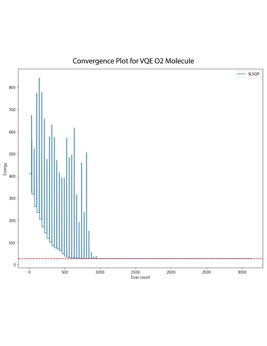
We plot some of the potentials in figures 7 and 8. Tables 3, 4 and 3 contain the results for the VQE calculations using 4 qubits and the the oscillator basis. In all cases we found excellent agreement with the experimentally measured values. Convergence plots for the VQE calculations are given in figures 9 and 10 and all cases rapidly converge near the ground state energy.

The Morse potential can be extended to treat triatomic molecules as well [14][15]. In this case the Morse potential depends on two coordinates $x,y$ and Hamiltonian can be written as :

$${H_{1}}=\frac{{p_{x}^{2}}}{{2m}}+\frac{{p_{y}^{2}}}{{2m}}-\frac{{{p_{x}}{p_{y}}}}{M}+C{\left({1-{e^{-x/b}}}\right)^{2}}+C{\left({1-{e^{-y/b}}}\right)^{2}}$$

(5.1)

Another form of the Hamiltonian can be formed by changing variables

$$x=({x_{1}}+{x_{2}})/\sqrt{2}$$

$$y=({x_{1}}-{x_{2}})/\sqrt{2}$$

(5.2)

and defining

$${m_{1}}=\frac{m}{{1-\frac{m}{M}}}$$

$${m_{2}}=\frac{m}{{1+\frac{m}{M}}}$$

(5.3)

In this form of the Hamiltonian can be written:

$${H_{2}}=\frac{{p_{1}^{2}}}{{2{m_{1}}}}+\frac{{p_{2}^{2}}}{{2{m_{2}}}}+C{\left({1-{e^{-\left({{x_{1}}+{x_{2}}}\right)/\sqrt{2}b}}}\right)^{2}}+C{\left({1-{e^{-\left({{x_{1}}-{x_{2}}}\right)/\sqrt{2}b}}}\right)^{2}}$$

(5.4)

A plot of this potential is given in Figure 12. For the case $m=1$, $M=2$, $C=10$ and $b=\sqrt{20}$, we find the ground state energy $E_{0}=0.954585$ using either Hamiltonian. Defining the tensor product operators

$${X_{1}}={X_{osc}}\otimes I$$

$${X_{2}}=I\otimes{X_{osc}}$$

$${P_{1}}={P_{osc}}\otimes I$$

$${P_{2}}=I\otimes{P_{osc}}$$

(5.5)

and using 8 qubits for the definition of the Hamiltonian in Equation 5.1, we find $E_{0}=0.957527$ using the VQE algorithm. A table of the simulation parameters and results for both $H_{1}$ and $H_{2}$ are presented in Table 6. The variational form for both simulations is shown in Figure 11.

In this paper we investigated using a quantum computer to simulate Hamiltonians using the Morse potential for supersymmetric quantum mechanics, diatomic molecules and triatomic molecules. In all cases we found excellent agreement with the exact answers using IBM QISKit and its statevector simulator. It will be interesting to extend these calculations to other molecules and combine these methods with electronic structure calculations on near term quantum computers which can determine the parameters of the Morse potential [16][17]. This approach was used in [18] to compute thermodynamic observables of the molecular systems. Finally it is important to study other variational forms as well as error and noise mitigation on near term devices associated with the calculations of the Morse potential to gain further understanding of the applicability of this effective Hamiltonian approach for molecules. The effective Hamiltonian approach may prove quite useful for molecular systems for which electronic structure calculations are too expensive on existing quantum hardware.

References

- [1] P. M. Morse, “Diatomic Molecules According to the Wave Mechanics. 2. Vibrational Levels,” Phys. Rev. 34, 57 (1929). doi:10.1103/PhysRev.34.57
- [2] E. Witten, “Dynamical Breaking of Supersymmetry,” Nucl. Phys. B 188, 513 (1981). doi:10.1016/0550-3213(81)90006-7
- [3] F. Cooper, A. Khare and U. Sukhatme, “Supersymmetry and quantum mechanics,” Phys. Rept. 251, 267 (1995) doi:10.1016/0370-1573(94)00080-M [hep-th/9405029].
- [4] A. Gangopadhyaya, J. V. Mallow and C. Rasinariu, “Supersymmetric Quantum Mechanics : An Introduction,” doi:10.1142/10475
- [5] I. Cooper, ”An integrated approach to ladder and shift operators for the Morse oscillator, radial Coulomb and radial oscillator potentials”, J. Phys. A: Math. Gen. 26, 1601 (1993).
- [6] G. Junker, P. Roy, ”Supersymmetric construction of exactly solvable potentials and nonlinear algebras”, Physics of atomic nuclei 61, 1736 (1998).
- [7] M. Arik, M. Baykal, A. Baykal, ”Factorization method for d-dimensional isotropic harmonic oscillator and the generalized Laguerre polynomials”, arxiv:0808.2289
- [8] M. Berrondo, A. Palma,J. Loez-BonillA, ”Matrix elements for the Morse potential using ladder operators”, Int.J.Quant.Chem. 31, 243 (1987).
- [9] R. Miceli, M. McGuigan ”Quantum computation and visualization of Hamiltonians using discrete quantum mechanics and IBM QISKit”, Proc. New York Scientific Data Summit, arXiv:1812.01044 [quant-ph] (2018).
- [10] P. Okock, ”A Matrix Method for Solving the Schrodinger Equation” Masters Thesis (2015).
- [11] H. Korsch, M. Gluck, ”Computing Eigenvalues Made Easy”, Eur. J. Phys. 23 (2002).
- [12] J. Motycka, J. Urban, P. Babinec, ”Eigenvalues of supersymmetric matrix models”, Act. Phys.Pol. B 45, 1743 (2014).
- [13] E. Fidiani, Modeling of diatomic molecules using the Morse potential and the Verlet algorithm, AIP Conference Proceeding 1719, 030001 (2016)
- [14] A. Bordoni, ”Systematic calculation of molecular spectra through a complete Morse expansion”.
- [15] J. Chesick, ”Gaussian basis sets for model anharmonic oscillator systems”, J. Chem. Phys. 49, 3772 (1968).
- [16] V. Armaos, D. Badounas, P.Deligiannis, K. Lianos, ”Computational Chemistry on Quantum Computers: Ground State Estimation”, Appl. Phys. A. 126, 625 arXiv:1907.00362 [quant-ph] (2020).
- [17] K.Choo, A. Mezzacapo, G. Carleo, ”Fermionic neural-network states for ab-initio electronic structure”, arXiv:1909.12852 [physics.comp-ph] (2019).
- [18] S. Stober, S. Harwood, D. Greenberg, Y. Gujarati, S. Mostame, S. Raman, T. Trenev, ”Computing thermodynamic observables on noisy quantum computers with chemical accuracy”, arXiv:2003.02303 [physics.chem-ph] (2020).