Current induced by a tilted magnetic field in phosphorene under terahertz laser radiation

Since its discovery in 2004, graphene research has observed exponential growth and has founded a new era in nanomaterials, and their applications (novoselov2004electric; geim2010rise; novoselov2012roadmap). The revolutionary discovery has triggered a pursuit for two–dimensional (2D) materials beyond graphene (butler2013progress). Subsequently, a series of monolayer 2D materials have been produced from graphene to transition metal dichalcogenides (TMDCs), and phosphorene (huo20152d; shim2017electronic; akhtar2017recent; peruzzini2019perspective). These materials have diverse electronic and optical properties. For instance, graphene is a zero–bandgap semiconductor, while phosphorene has a $2$ $\mathrm{eV}$ natural bandgap. Also, the bandgaps observed in most TMDCs are larger than $1$ $\mathrm{eV}$. Therefore, different materials in the 2D domain present diverse electronic and optoelectronic applications.

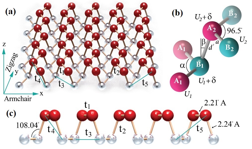
In this study, we investigate phosphorene, the monolayer of black–phosphorus (Fig. 1(a)). Several motivations exist for studying phosphorene’s response to THz laser radiation. First, in phosphorene, carrier mobility is much higher than other 2D materials such as TMDCs ($\leq 200$ $\mathrm{cm^{2}V^{-1}s^{-1}}$). Also, phosphorene is comparable to graphene in its electron conduction rate ($650$ $\mathrm{cm^{2}V^{-1}s^{-1}}$ at room temperature). This characteristic makes phosphorene a desirable material for high–frequency electronics (dhanabalan2017emerging; viti2015black; xia2014rediscovering). Second, though the large dark currents that dominate under a non–zero bias operation restrict graphene’s performance, phosphorene’s direct bandgap makes it a suitable choice in high–frequency optoelectronics, ultra–fast photonics, transparent photovoltaics, and photodetection (viti2015black; gan2013chip; koppens2014photodetectors; luo2015microfiber; sun2016optical). Undeniably, phosphorene’s $I_{on}/I_{off}$ ratio of $~10^{5}$ make it an appropriate choice for detecting THz frequency radiation (das2014tunable; viti2015black). Third, every phosphorus atom in phosphorene has a covalent bond with three adjacent phosphorus atoms. Hence, each of the $p$ orbitals holds a single pair of electrons. Unlike graphene, $sp^{3}$ hybridization prevents phosphorene from forming an atomically flat sheet. The latter characteristic produces an intrinsic in–plane anisotropy, which deduces to an explicitly angle-dependent conductivity (viti2015black). Phosphorene’s puckered structure deduces to a strong anisotropy in electrical conductivity, and it is important to have novel devices with anisotropic properties. (sun2016optical). This is while the photonic and electronic properties of graphene and TMDCs are largely isotropic and do not exhibit a significant directional dependence (xia2014rediscovering; peruzzini2019perspective). Fourth, phosphorene is an inorganic material easily integrated with photonic or optoelectronic 2D materials, such as graphene or silicon–based materials (viti2015black). For these reasons, we selected phosphorene to investigate the linear and nonlinear responses of a 2D anisotropic material subjected to THz laser radiation. Ultrafast signal processing largely relies on nonlinear optics in which the higher power of the electric field determines the strength of the response. Although recent studies have studied graphene in the context of the linear and nonlinear transport effects in electric fields (kheirabadi2018cyclotron; kheirabadi2016magnetic; drexler2013magnetic; glazov2014high; olbrich2016terahertz), the linear and nonlinear current response in phosphorene has seldom been investigated (kheirabadi2020magnetic). This study aims to examine the current response of phosphorene subjected to a steady magnetic field. The present study results offer a new perspective on the anisotropic nonlinear optical properties of an anisotropic 2D material with possible applications in polarized optics, optical switching, and photodetection. The latter relies on the conversion of absorbed photons into an electrical signal that is probably the most explored black–phosphorus based photonic device (guo2016black). The calculations provided in this study are valid for $\hbar\omega\leq\epsilon_{f}$ where $\omega$ is the angular frequency of laser radiation, and $\epsilon_{f}$ is the Fermi level; semi–classical regime. Therefore, the study’s results are suitable for application in THz– and microwave– optoelectronic devices.

In this study, we demonstrate that subjected to a steady tilted magnetic field and THz laser radiation, a first-order AC current, a second-order DC current (ratchet effect), and a second-order AC current (second harmonic generation (SHG)) is deduced in phosphorene. The ratchet effect is a nonlinear response to a driving light field that results in a DC current. SHG is a second-order in electric field effect by which an AC current with two times the frequency related to the incoming AC radiation is generated. Also, due to an existing perpendicular magnetic field, the cyclotron resonance impacts the deduced currents’ strength in phosphorene. The cyclotron resonance of the magnetic ratchet effect and SHG have been investigated in isotropic materials such as 2D electron gas (budkin2016ratchet), and bilayer graphene (kheirabadi2018cyclotron). The effect is yet to be investigated in anisotropic materials, such as phosphorene, which we will examine in this study.

We derived the tight–binding Hamiltonian of phosphorene under the effect of an in–plane magnetic field (kheirabadi2020magnetic). The Hamiltonian of phosphorene in a steady in–plane magnetic field and in the basis of $(A_{1},B_{1},A_{2},B_{2})^{T}$ (Fig. 1(b)) is

$\displaystyle H=\begin{pmatrix}U_{1}&f_{1}+f_{3}&f_{4}&f_{2}+f_{5}\\ {f_{1}}^{*}+{f_{3}}^{*}&U_{1}+\delta&{f_{2}}^{*}+{f_{5}}^{*}&f_{4}\\ {f_{4}}^{*}&f_{2}+f_{5}&U_{2}+\delta&f_{1}^{\prime}+f_{3}^{\prime}\\ {f_{2}}^{*}+{f_{5}}^{*}&{f_{4}}^{*}&{f_{1}^{\prime}}^{*}+{f_{3}^{\prime}}^{*}&U_{2}\end{pmatrix}.$

We assume that $\textbf{b}=ed\textbf{B}_{\parallel}/2$ where $-e$ is the electron charge, $d$ is the interlayer distance, $\textbf{B}_{\parallel}$ is the in–plane magnetic field, in–plane momentum is $\mathbf{p}=(p_{x},p_{y},0)$, different on-site energies are $U_{1}$ and $U_{2}$, $\delta$ is the interlayer potential asymmetry, and $a_{x}$ and $a_{y}$ are the length of the unit cell into the $x$ (armchair) and $y$ (zigzag) directions, respectively (Fig. 1(a and b)). Hence, we have

	$\displaystyle f_{1}$		$\displaystyle=2t_{1}\cos{\frac{a_{y}(p_{y}+b_{x})}{2\hbar}}\mathrm{exp}{\big[\frac{i(p_{x}-b_{y})}{\hbar}a\cos{\frac{\alpha}{2}}}\big],$
	$\displaystyle f_{1}^{\prime}$		$\displaystyle=2t_{1}\cos{\frac{a_{y}(p_{y}-b_{x})}{2\hbar}}\mathrm{exp}{\big[\frac{i(p_{x}+b_{y})}{\hbar}a\cos{\frac{\alpha}{2}}}\big],$
	$\displaystyle f_{2}$		$\displaystyle=t_{2}\mathrm{exp}[-\frac{i}{\hbar}p_{x}d^{\prime}\sin\beta],$
	$\displaystyle f_{3}$		$\displaystyle=2t_{3}\cos{\frac{a_{y}(p_{y}+b_{x})}{2\hbar}}$
			$\displaystyle\quad\times\mathrm{exp}{\big[-\frac{i(p_{x}-b_{y})}{\hbar}(2d^{\prime}\sin\beta+a\cos{\frac{\alpha}{2})}}\big],$
	$\displaystyle f_{3}^{\prime}$		$\displaystyle=2t_{3}\cos{\frac{a_{y}(p_{y}-b_{x})}{2\hbar}}$
			$\displaystyle\quad\times\mathrm{exp}{\big[-\frac{i(p_{x}+b_{y})}{\hbar}(2d^{\prime}\sin\beta+a\cos{\frac{\alpha}{2})}}\big],$
	$\displaystyle f_{4}$		$\displaystyle=4t_{4}\cos[\frac{p_{x}}{\hbar}(d^{\prime}\sin\beta+a\cos\frac{\alpha}{2})]\cos[\frac{p_{y}}{\hbar}a\sin\frac{\alpha}{2}],$
	$\displaystyle f_{5}$		$\displaystyle=t_{5}\mathrm{exp}[i\frac{p_{x}}{\hbar}(a_{x}-d^{\prime}\sin\beta)].$

In the above-mentioned equations, the intralayer coupling is $t_{1}$, the interlayer couplings are $t_{2}$, $t_{4}$ and $t_{5}$, $d^{\prime}$ is the distance between $B_{1}$ and $A_{2}$ atoms, $\alpha$ is $\widehat{A_{1}B_{1}A_{1}}=\widehat{B_{2}A_{2}B_{2}}=96.5^{\circ}$, $\beta$ is $\widehat{A_{2}B_{1}A_{1}}-90^{\circ}=108.04^{\circ}-90^{\circ}=18.04^{\circ}$ (chaves2017theoretical; pereira2015landau) (Fig. 1(c)), the upper layer is located at $d/2$, and the lower layer is located at $-d/2$ (Fig. 1). Based on this Hamiltonian and according to the perturbation theory, we can derive the perturbed valence and conduction bands (kheirabadi2020magnetic; kheirabadi2016magnetic). By this assumption, we have considered the orbital effect of an in–plane magnetic field on the electrons. Furthermore, we assume that the redistribution of charge carriers in the momentum and energy space is induced by an in–plane laser radiation incident on the phosphorene plane. Consequently, we assume that the applied AC electric field of THz laser radiation is

$$\mathbf{E}_{\parallel}(t)=\mathbf{E}_{\parallel}\mathrm{exp}(-i\omega t)+\mathbf{E}_{\parallel}^{*}\mathrm{exp}(i\omega t),$$

where $\mathbf{E}_{\parallel}=(E_{x},E_{y})$, and $\mathbf{E}_{\parallel}^{*}=(E_{x}^{*},E_{y}^{*})$.

Out of an equilibrium condition caused by the laser radiation, the electron distribution function is dependent on the momentum $\mathbf{p}$ and time $t$; $f(\mathbf{p},t)$. If we consider that the system under study is spatially homogeneous, $f(\mathbf{p},t)$ satisfies the following Boltzmann kinetic equation

$\displaystyle-e\bigg(\mathbf{E}_{\parallel}+\mathbf{V}_{g}\times\mathbf{B}_{\perp}\bigg)\cdot\mathbf{\triangledown}_{p}f(\mathbf{p},t)+\frac{\partial f(\mathbf{p},t)}{\partial t}=S\{f\}\ ,$

where the group velocity is $\mathbf{V}_{g}=V_{g,x}\cos\phi\mathbf{\hat{i}}+V_{g,y}\sin\phi\mathbf{\hat{j}}$, $\phi$ is the polar angle of momentum, $\mathbf{B}_{\perp}$ is the perpendicular magnetic field, and $S\{f\}$ is the collision integral. Also, $V_{g,x}=p/m_{xx}$ and $V_{g,y}=p/m_{yy}$, where $p={\left|\textbf{p}\right|}$, $m_{xx}$ and $m_{yy}$ are effective mass along the $x$ and $y$ directions, respectively (lowrelax). To solve the Boltzmann equation, Eq. II, we consider the distribution function as the following series

$$f(\mathbf{p},t)=\sum_{n,m}f_{m}^{n}e^{im\phi-in\omega t},$$

where $f_{m}^{n}$ coefficients are functions of the total energy of an electron, $\epsilon$, and m and n are integers. Then, we multiply the Boltzmann equation in $\mathrm{exp}(-ij\phi+il\omega t)$, where $j$ and $l$ are integers and integrate over a period of $2\pi$ of angle $\phi$ and a period of time; $t$. Therefore, coupled equations between different $f_{m}^{n}$ coefficients are achieved in the following form

	$\displaystyle\gamma^{l,j}f_{j}^{l}$		$\displaystyle=\alpha_{j-1}f_{j-1}^{l-1}+\widetilde{\alpha}_{j-1}f_{j-1}^{l+1}+\beta_{j+2}f^{l}_{j+2}$		(2)
			$\displaystyle+\widetilde{\beta}_{j-2}f^{l}_{j-2}+\eta_{j+1}f_{j+1}^{l-1}+\widetilde{\eta}_{j+1}f_{j+1}^{l+1}+\delta S_{j}^{l}.$

In Eq. 2, $\gamma^{l,j}=\tau_{\left|j\right|,\mathbf{p}}^{-1}-il\omega+ij\omega_{c_{+}}$, where $\tau_{\left|j\right|,\mathbf{p}}^{-1}$ is the relaxation time of the jth angular harmonic of the electron distribution function, $\omega_{c_{+}}=eB_{\perp}/(2m_{+})$ is the cyclotron frequency including the cyclotron resonance effect, and $1/m_{+}=1/m_{xx}+1/m_{yy}$. Also, linear in electric field $\alpha$, $\beta$, and $\eta$ operators are

	$\displaystyle\alpha_{j}$		$\displaystyle=\frac{e(E_{x}-iE_{y})}{2}\left(-\frac{j}{p}+\frac{\partial}{\partial p}\right),$
	$\displaystyle\tilde{\alpha}_{j}$		$\displaystyle=\frac{e(E_{x}^{*}-iE_{y}^{*})}{2}\left(-\frac{j}{p}+\frac{\partial}{\partial p}\right),$
	$\displaystyle\beta_{j}$		$\displaystyle=\frac{1}{2}\omega_{c_{-}}\big(ip\frac{\partial}{\partial p}+j\big),$
	$\displaystyle\widetilde{\beta}_{j}$		$\displaystyle=\frac{1}{2}\omega_{c_{-}}\big(-ip\frac{\partial}{\partial p}+j\big),$
	$\displaystyle\eta_{j}$		$\displaystyle=\frac{e(E_{x}+iE_{y})}{2}\left(\frac{j}{p}+\frac{\partial}{\partial p}\right),$
	$\displaystyle\tilde{\eta}_{j}$		$\displaystyle=\frac{e(E_{x}^{*}+iE_{y}^{*})}{2}\left(\frac{j}{p}+\frac{\partial}{\partial p}\right).$

Here, we have $\omega_{c_{-}}=eB_{\perp}/(2m_{-})$ and $1/m_{-}=1/m_{xx}-1/m_{yy}$. In Eq. 2, $\delta S_{j}^{l}$ is the correction to the scattering caused by an in–plane magnetic field.

For an anisotropic 2D electron gas such as phosphorene, where $\xi$ is the unit matrix of the electric field, the relaxation time of the jth angular harmonic, $\tau_{\left|j\right|,\mathbf{p}}^{-1}$, is (relaxtime; lowrelax)

	$\displaystyle\tau^{-1}_{\left|j\right|,\mathbf{p}}(\mathbf{\xi},\mathbf{p})$		$\displaystyle=\frac{2\pi}{\hbar}\sum_{\mathbf{p}^{\prime}}\left|\langle\mathbf{p^{\prime}}\left|\delta H\right|\mathbf{p}\rangle\right|^{2}\delta\left(\epsilon_{p}-\epsilon_{p^{\prime}}\right)$		(3)
			$\displaystyle\quad\times\left\{1-\frac{[\mathbf{\xi}.\mathbf{V}_{g}(\mathbf{p^{\prime}})]\tau_{\left|j\right|,\mathbf{p^{\prime}}}}{[\mathbf{\xi}.\mathbf{V}_{g}(\mathbf{p})]\tau_{\left|j\right|,\mathbf{p}}}\right\}.$

Note that for isotropic materials, we have $\omega_{c_{-}}=0$ and $\omega_{c_{+}}=eBV_{g}/p$ and $\tau_{\left|j\right|,\mathbf{p}}(\mathbf{\xi},\mathbf{p})=\tau_{\left|j\right|}$. So, Eq. 2 and 3 are also valid for isotropic materials (budkin2016ratchet; olbrich2013giant; dantscher2015cyclotron; kheirabadi2018cyclotron).

For static impurities, we can show that (kheirabadi2016magnetic; kheirabadi2018cyclotron; kheirabadi2020magnetic)

$\displaystyle\delta H=\sum_{j=1}^{N_{imp}}\hat{Y}u(\mathbf{r}-\mathbf{R_{j}}),$

(4)

where $N_{imp}$ is the number of impurities, $u(\mathbf{r}-\mathbf{R_{j}})$ describes the spatial dependence of the impurity potential and $\hat{Y}$ is a dimensionless matrix describing the additional degree of freedom related to the structure within the unit cell. We neglect the interference between different impurities and employ the Fourier transform of the impurity potential and perform a harmonic expansion of the impurity potential; so, we have

$\displaystyle\lvert\tilde{u}(\mathbf{p^{\prime}-p})\rvert^{2}=\sum_{m^{\prime}}\nu_{m^{\prime}}e^{im^{\prime}(\phi^{\prime}-\phi)}.$

In addition, we assume that the electrons are trapped in a huge box with the length $L$ and under a periodic potential. Hence, the current density is

$\displaystyle\mathbf{J}=-\frac{g}{L^{2}}\sum_{\mathbf{p}}e\mathbf{V}_{g}f(\mathbf{p},t),$

where $g$ is the spin degeneracy factor $(g=2)$. In thermal equilibrium, and wherever there is no electric field, only the $f_{0}^{0}$ harmonic generated by the Fermi–Dirac distribution function is nonzero. However, when an AC electric field is applied to the system, other harmonics arise, and this gives the possibility of having a linear (first-order) or nonlinear (higher orders) in electric field currents. In this study, we consider all nonzero first order or second order in electric field currents. Hence, based on coupled equations (Eq. 2), $f_{j}^{l}$ harmonics in terms of the equilibrium distribution function ($f_{0}^{0}$) should be calculated. In addition, we assume that the system is a degenerate electron gas at low temperature condition; so, we have $\partial f_{0}^{0}/\partial\epsilon\approx-\delta(\epsilon-\epsilon_{f})$.

To find $f_{j}^{l}$ harmonics in Eq. 2, first, we should find the correction to the scattering caused by the in–plane magnetic field, $\delta S_{j}^{l}$. We have

	$\displaystyle\delta S_{j}^{l}$		$\displaystyle=L^{2}\int_{0}^{\infty}\bigg[\sum_{m}f_{m}^{l}\Gamma(\epsilon)d\epsilon$
			$\displaystyle\times\int_{0}^{2\pi}\delta W_{\mathbf{p^{\prime}}\mathbf{p}}\bigg(e^{im\phi^{\prime}-ij\phi}-e^{im\phi-ij\phi}\bigg)\frac{d\phi}{2\pi}\frac{d\phi^{\prime}}{2\pi}\bigg],$

where $\Gamma(\epsilon)$ is the electronic density of states per spin and per unit area and $\delta W_{\mathbf{p^{\prime}}\mathbf{p}}$ is the change of the scattering rate caused by the in–plane magnetic field. The scattering rate of an electron passes through a phosphorene in a steady magnetic field to the linear order in $\mathbf{B}_{\parallel}$ and momentum is calculated before (kheirabadi2020magnetic). Accordingly, for the case of the asymmetric disorder where the lower layer ($\zeta=1$) or the upper layer ($\zeta=-1$) symmetry is broken by the disorder ($z\rightarrow-z$ asymmetry), $\hat{Y}$ in Eq. 4 is equal to $\big(\hat{I}+\zeta\hat{\sigma_{z}}\otimes\hat{I}\big)/2$, where $\hat{I}$ is the $2\times 2$ unit matrix, and $\sigma_{z}$ is a Pauli matrix. Consequently, $\delta W_{\mathbf{p^{\prime}}\mathbf{p}}$ has the following general form:

	$\displaystyle\delta W_{\mathbf{p^{\prime}}\mathbf{p}}(\zeta,U_{1},U_{2},\delta)$		$\displaystyle=\frac{2\pi}{\hbar}\frac{n_{imp}}{L^{2}}\lvert\tilde{u}(\bf{p}^{\prime}-\bf{p})\rvert^{2}\delta(\epsilon_{p^{\prime}}-\epsilon_{p})$
			$\displaystyle\times\bigg\{\frac{1}{\hbar^{2}}C_{1}(\zeta,U_{1},U_{2},\delta)b_{y}p(\cos\phi+\cos\phi^{\prime})$
			$\displaystyle+\frac{1}{\hbar^{2}}C_{2}(\zeta,U_{1},U_{2},\delta)b_{x}p(\sin\phi+\sin\phi^{\prime})\bigg\}.$

In Eq. III, the $n_{imp}=N_{imp}/L^{2}$, $C$ coefficients are dependent on on–site energies and disorder types. Consequently, according to Eq. III, we can show that

	$\displaystyle\delta S_{0}^{l}$		$\displaystyle=0,$
	$\displaystyle\delta S_{1}^{l}$		$\displaystyle=\Lambda\big(C_{1}B_{y}+iC_{2}B_{x}\big)f_{2}^{l},$
	$\displaystyle\delta S_{-1}^{l}$		$\displaystyle=\Lambda\big(C_{1}B_{y}-iC_{2}B_{x}\big)f_{-2}^{l},$
	$\displaystyle\delta S_{2}^{l}$		$\displaystyle=\Lambda\big(C_{1}B_{y}-iC_{2}B_{x}\big)f_{1}^{l},$
	$\displaystyle\delta S_{-2}^{l}$		$\displaystyle=\Lambda\big(C_{1}B_{y}+iC_{2}B_{x}\big)f_{-1}^{l},$

where $\Lambda=ed\pi n_{imp}\Omega\Gamma(\epsilon)p/2\hbar^{3}$ and $\Omega=-(\nu_{0}-\nu_{2})$.

The first order AC current is the result of $f_{1}^{1}$ and $f_{-1}^{1}$ harmonics and the complex conjugate of those terms; $f_{m}^{n}=\big(f_{-m}^{-n}\big)^{*}$. We can show that the first order AC current is

$$\mathbf{J}=2Re\{\sigma\mathbf{E}e^{-i\omega t}\},$$

where $\sigma$ is the conductivity tensor. The conductivity tensor components are $\sigma_{ii}=\sigma_{0i}\sigma^{\prime}_{ii}$ and $\sigma_{ij}=\sigma_{0i}\sigma^{\prime}_{ij}$, where $i$ and $j$ indicate the $x$ or $y$ directions and

$\displaystyle\sigma_{0i}$

$\displaystyle=\frac{ge^{2}}{2}\Gamma(\epsilon)C_{ph}pV_{g,i},$

(7)

$\displaystyle\sigma^{\prime}_{xx}=\sigma^{\prime}_{yy}$

$\displaystyle=\frac{(1-i\omega\tau_{1,\mathbf{p}})\tau_{1,\mathbf{p}}}{(1-i\omega\tau_{1,\mathbf{p}})^{2}+(\omega_{c_{+}}\tau_{1,\mathbf{p}})^{2}},$

(8)

$\displaystyle\sigma^{\prime}_{xy}=-\frac{(\omega_{c_{+}}+\omega_{c_{-}}+i\omega_{c_{-}}/2)\tau^{2}_{1,\mathbf{p}}}{(1-i\omega\tau_{1,\mathbf{p}})^{2}+(\omega_{c_{+}}\tau_{1,\mathbf{p}})^{2}}$

(9)

$\displaystyle\sigma^{\prime}_{yx}$

$\displaystyle=\frac{(\omega_{c_{+}}-\omega_{c_{-}}-i\omega_{c_{-}}/2)\tau^{2}_{1,\mathbf{p}}}{(1-i\omega\tau_{1,\mathbf{p}})^{2}+(\omega_{c_{+}}\tau_{1,\mathbf{p}})^{2}}$

(10)

Here, we have $\omega_{c_{+}}+\omega_{c_{-}}=eB_{\perp}/m_{xx}$ and $\omega_{c_{+}}-\omega_{c_{-}}=eB_{\perp}/m_{yy}$. These calculations are valid for a degenerate electron gas, $\epsilon_{f}\gg k_{B}T$. All the parameters are evaluated on the Fermi surface and the above–mentioned results are in agreement with those related to isotropic materials (kheirabadi2018cyclotron). In Eq. 7, we have

	$\displaystyle\frac{\partial}{\partial p}$		$\displaystyle=C_{ph}p\frac{\partial}{\partial\epsilon},$
	$\displaystyle C_{ph}$		$\displaystyle=s\frac{2}{\hbar^{2}}\bigg[\frac{\gamma^{2}}{E_{g}}+\big(\eta_{v/c}+\nu_{v/c}\big)\bigg],$

where $s$ is the band index, and it is $+1$ for the conduction band and $-1$ for the valence band. $E_{g}$ is the direct energy gap, $E_{g}=0.912$ $\mathrm{eV}$, $\gamma=0.480$ $\mathrm{eVnm}$, $\eta_{v}=0.038$ $\mathrm{eVnm^{2}}$, $\nu_{v}=0.030$ $\mathrm{eVnm^{2}}$, $\eta_{c}=0.008$ $\mathrm{eVnm^{2}}$, and $\nu_{c}=0.030$ $\mathrm{eVnm^{2}}$ are from Ref. (AsgariHamil).

According to Eqs. 8 to 10, there are resonances at $\omega=\pm\omega_{c_{+}}$. At these frequencies, the current is much larger than at $\omega_{c_{+}}=0$.

The ratchet effect is a nonlinear response to a driving light field where $f_{1}^{0}$ and $f_{-1}^{0}$ harmonics result in a DC current. The ratchet current is calculated based on the following equation:

$$\mathbf{J}=-\frac{ge}{L^{2}}\sum_{\mathbf{p}}\mathbf{V}_{g}\big(f_{1}^{0}e^{i\phi}+f_{-1}^{0}e^{-i\phi}\big).$$

For $\Theta_{1}=\lvert E_{x}\rvert^{2}-\lvert E_{y}\rvert^{2}$, $\Theta_{2}=E_{x}E_{y}^{*}+E_{x}^{*}E_{y}$, and $\Theta_{3}=i\big(E_{x}E_{y}^{*}-E_{x}^{*}E_{y}\big)$, we can show that the current is

	$\displaystyle J_{x}$		$\displaystyle=\lvert{E}\rvert^{2}\big(B_{y}^{\prime}Re[M_{2,x}]+B_{x}^{\prime}Im[M_{2,x}]\big)$
			$\displaystyle+\Theta_{1}\big(B_{y}^{\prime}Re[M_{1,x}]-B_{x}^{\prime}Im[M_{1,x}]\big)$
			$\displaystyle+\Theta_{2}\big(B_{y}^{\prime}Im[M_{1,x}]+B_{x}^{\prime}Re[M_{1,x}]\big)$
			$\displaystyle+\Theta_{3}\big(B_{y}^{\prime}Re[M_{3,x}]+B_{x}^{\prime}Im[M_{3,x}]\big),$

	$\displaystyle J_{y}$		$\displaystyle=\lvert{E}\rvert^{2}\big(-B_{y}^{\prime}Im[M_{2,y}]+B_{x}^{\prime}Re[M_{2,y}]\big)$
			$\displaystyle-\Theta_{1}\big(B_{y}^{\prime}Im[M_{1,y}]+B_{x}^{\prime}Re[M_{1,y}]\big)$
			$\displaystyle+\Theta_{2}\big(B_{y}^{\prime}Re[M_{1,y}]-B_{x}^{\prime}Im[M_{1,y}]\big)$
			$\displaystyle+\Theta_{3}\big(-B_{y}^{\prime}Im[M_{3,y}]+B_{x}^{\prime}Re[M_{3,y}]\big),$

where $B_{x}^{\prime}=C_{2}B_{x}$ and $B_{y}^{\prime}=C_{1}B_{y}$. In addition, the $M$ coefficients are

	$\displaystyle M_{1,i}$		$\displaystyle=-\frac{ge^{3}}{4}C_{ph}p\big(\frac{1}{\gamma^{-1,1}}+\frac{1}{\gamma^{1,1}}\big)$
			$\displaystyle\times\bigg\{\frac{V_{g,i}\Lambda}{\gamma^{0,1}\gamma^{0,2}p}\Gamma(\epsilon)+C_{ph}(\Gamma(\epsilon)\frac{V_{g,i}\Lambda}{\gamma^{0,1}\gamma^{0,2}}p\big)^{\prime}\bigg\},$

	$\displaystyle M_{2,i}$		$\displaystyle=\frac{ge^{3}}{4}C_{ph}p\Lambda\big(\frac{1}{\gamma^{-1,2}\gamma^{-1,1}}+\frac{1}{\gamma^{1,2}\gamma^{1,1}}\big)$
			$\displaystyle\times\bigg\{\frac{2V_{g,i}}{\gamma^{0,1}p}\Gamma(\epsilon)-C_{ph}(\Gamma(\epsilon)\frac{V_{g,i}}{\gamma^{0,1}}p\big)^{\prime}\bigg\},$

	$\displaystyle M_{3,i}$		$\displaystyle=\frac{ge^{3}}{4}C_{ph}p\Lambda\big(\frac{1}{\gamma^{1,2}\gamma^{1,1}}-\frac{1}{\gamma^{-1,2}\gamma^{-1,1}}\big)$
			$\displaystyle\times\bigg\{\frac{2V_{g,i}}{\gamma^{0,1}p}\Gamma(\epsilon)-C_{ph}(\Gamma(\epsilon)\frac{V_{g,i}}{\gamma^{0,1}}p\big)^{\prime}\bigg\},$

where $(\ldots)^{\prime}\equiv\partial(\ldots)/\partial\epsilon$ and all parameters are evaluated on the Fermi surface. Also, for $\omega_{c_{+}}=0$, where the perpendicular magnetic field is zero, the above results are in agreement with previous results (kheirabadi2020magnetic).

Moreover, $M_{1,i}$ is the response to the linearly polarized light, $M_{2,i}$ is the response to the unpolarized light, and $M_{3,i}$ is the response to the circularly polarized light. For linearly polarized light, we can assume that $E_{x}^{*}=E_{x}=(E_{0}/2)\cos{\theta}$ and $E_{y}^{*}=E_{y}=(E_{0}/2)\sin{\theta}$, where $\theta$ is the polarization angle. We also assume that $B^{\prime}_{\parallel}=\big({B^{\prime}_{x}}^{2}+{B^{\prime}_{y}}^{2}\big)^{1/2}$ and $\varphi^{\prime}=\arctan\big(B^{\prime}_{y}/B^{\prime}_{x}\big)$. For linearly polarized light, we can show that the currents in the $x$ and $y$ directions are

	$\displaystyle J_{x}$		$\displaystyle=\frac{E_{0}^{2}}{4}B_{\parallel}^{\prime}\bigg\{\left\lvert M_{2,x}\right\rvert\sin(\varphi^{\prime}+\chi_{2,x})$		(11)
			$\displaystyle\quad\quad\quad\quad+\left\lvert M_{1,x}\right\rvert\cos(2\theta+\varphi^{\prime}-\chi_{1,x}+\frac{\pi}{2})\bigg\},$
	$\displaystyle J_{y}$		$\displaystyle=\frac{E_{0}^{2}}{4}B_{\parallel}^{\prime}\bigg\{\left\lvert M_{2,y}\right\rvert\cos(\varphi^{\prime}+\chi_{2,y})$		(12)
			$\displaystyle\quad\quad\quad\quad+\left\lvert M_{1,y}\right\rvert\sin(2\theta+\varphi^{\prime}-\chi_{1,y}+\frac{\pi}{2})\bigg\},$

where $\chi_{1,i}=arg(M_{1,i})$ and $\chi_{2,i}=arg(M_{2,i})$. For unpolarized light, $M_{1,i}$ related terms are equal to zero, but $M_{2,i}$ related terms survive. In addition, $M_{1,i}$ related current has a notable resonance for $\omega=\pm\omega_{c_{+}}$ and the strength of the ratchet effect is highest for $\omega_{c_{+}}=0$ (Fig. 2). Current induced by unpolarized light, $M_{2,i}$ has resonances for $\omega=\pm 2\omega_{c_{+}}$ that deduces to a DC current that is much larger in comparison to where $\omega_{c_{+}}=0$; $B_{\perp}=0$. The other resonance is related to $\omega=\pm\omega_{c_{+}}$. However, in this case, the deduced DC current is smaller than where $\omega_{c_{+}}=0$.

For circularly polarized light, we can show that $E_{x}^{*}=E_{x}=E_{0}/2$ and $E_{y}^{*}=-E_{y}=-i\mu E_{0}/2$, where $\mu=1(-1)$ for the left- (right-) handed circularly polarized light. For this radiation type, where $\chi_{3,i}=arg(M_{3,i})$, we can show that the current density is

	$\displaystyle J_{x}$		$\displaystyle=\frac{E_{0}^{2}}{2}B_{\parallel}^{\prime}\bigg\{\left\lvert M_{2,x}\right\rvert\sin(\varphi^{\prime}+\chi_{2,x})$		(13)
			$\displaystyle\quad\quad\quad\quad+\mu\left\lvert M_{3,x}\right\rvert\sin(\varphi^{\prime}+\chi_{3,x})\bigg\},$
	$\displaystyle J_{y}$		$\displaystyle=\frac{E_{0}^{2}}{2}B_{\parallel}^{\prime}\bigg\{\left\lvert M_{2,y}\right\rvert\cos(\varphi^{\prime}+\chi_{2,y})$		(14)
			$\displaystyle\quad\quad\quad\quad+\mu\left\lvert M_{3,y}\right\rvert\cos(\varphi^{\prime}+\chi_{3,y})\bigg\}.$

The above equations show that the response to circularly polarized light is dependent on the radiation helicity. For $M_{3,i}$, the major resonance effects are related to $\omega=\pm 2\omega_{c_{+}}$. There is also a resonance effect for $\omega=\pm\omega_{c_{+}}$ and both effects cause a current that is stronger than the current where $B_{\perp}=0$ (Fig. 2). According to Eqs. 11 to 14, the direction of the ratchet current for circularly and linearly polarized lights is dependent on the $\varphi^{\prime}$ and $\chi$ phases.

Assuming $\Theta_{4}=E_{x}^{2}-E_{y}^{2}$, and $\Theta_{5}=2E_{x}E_{y}$ and $\Theta_{6}=E_{x}^{2}+E_{y}^{2}$, we can show that the general current form for a degenerate electron gas is

	$\displaystyle J_{x}$		$\displaystyle=2Re\bigg\{\big[\Theta_{4}\big(N_{1,x}B_{y}^{\prime}+N_{2,x}B_{x}^{\prime}\big)$		(15)
			$\displaystyle\quad\quad\quad\quad+\Theta_{5}\big(-N_{2,x}B_{y}^{\prime}+N_{1,x}B_{x}^{\prime}\big)$
			$\displaystyle\quad\quad\quad\quad+\Theta_{6}\big(N_{3,x}B_{y}^{\prime}+N_{4,x}B_{x}^{\prime}\big)\big]e^{-2i\omega t}\bigg\},$
	$\displaystyle J_{y}$		$\displaystyle=2Re\bigg\{\big[\Theta_{4}\big(N_{2,y}B_{y}^{\prime}-N_{1,y}B_{x}^{\prime}\big)+\Theta_{5}\big(N_{1,y}B_{y}^{\prime}+N_{2,y}B_{x}^{\prime}\big)$		(16)
			$\displaystyle\quad\quad\quad\quad+\Theta_{6}\big(-N_{4,y}B_{y}^{\prime}+N_{3,y}B_{x}^{\prime}\big)\big]e^{-2i\omega t}\bigg\},$

$N$ coefficients in Eqs. 15 and 16 are

	$\displaystyle N_{1,i}$		$\displaystyle=-\frac{ge^{3}}{8}\big[V_{g,i}C_{ph}\Lambda\Gamma(\epsilon)\big(\frac{1}{\gamma^{2,1}\gamma^{2,2}\gamma^{1,1}}+\frac{1}{\gamma^{2,-1}\gamma^{2,-2}\gamma^{1,-1}}\big)$
			$\displaystyle\quad\quad\quad\quad+C_{ph}^{2}\frac{p}{\gamma^{1,1}}\big(\Gamma(\epsilon)\frac{V_{g,i}\Lambda}{\gamma^{2,1}\gamma^{2,2}}p\big)^{\prime}$
			$\displaystyle\quad\quad\quad\quad+C_{ph}^{2}\frac{p}{\gamma^{1,-1}}\big(\Gamma(\epsilon)\frac{V_{g,i}\Lambda}{\gamma^{2,-1}\gamma^{2,-2}}p\big)^{\prime}\big],$
	$\displaystyle N_{2,i}$		$\displaystyle=-\frac{ge^{3}}{8}i\big[V_{g,i}C_{ph}\Lambda\Gamma(\epsilon)\big(\frac{1}{\gamma^{2,1}\gamma^{2,2}\gamma^{1,1}}-\frac{1}{\gamma^{2,-1}\gamma^{2,-2}\gamma^{1,-1}}\big)$
			$\displaystyle\quad\quad\quad\quad+C_{ph}^{2}\frac{p}{\gamma^{1,1}}\big(\Gamma(\epsilon)\frac{V_{g,i}\Lambda}{\gamma^{2,1}\gamma^{2,2}}p\big)^{\prime}$
			$\displaystyle\quad\quad\quad\quad-C_{ph}^{2}\frac{p}{\gamma^{1,-1}}\big(\Gamma(\epsilon)\frac{V_{g,i}\Lambda}{\gamma^{2,-1}\gamma^{2,-2}}p\big)^{\prime}\big],$
	$\displaystyle N_{3,i}$		$\displaystyle=\frac{ge^{3}}{8}\big[2V_{g,i}C_{ph}\Lambda\Gamma(\epsilon)\big(\frac{1}{\gamma^{2,1}\gamma^{1,2}\gamma^{1,1}}+\frac{1}{\gamma^{2,-1}\gamma^{1,-2}\gamma^{1,-1}}\big)$
			$\displaystyle\quad\quad\quad\quad-C_{ph}^{2}\frac{p\Lambda}{\gamma^{1,2}\gamma^{1,1}}\big(\Gamma(\epsilon)\frac{V_{g,i}}{\gamma^{2,1}}p\big)^{\prime}$
			$\displaystyle\quad\quad\quad\quad-C_{ph}^{2}\frac{p\Lambda}{\gamma^{1,-2}\gamma^{1,-1}}\big(\Gamma(\epsilon)\frac{V_{g,i}}{\gamma^{2,-1}}p\big)^{\prime}\big],$
	$\displaystyle N_{4,i}$		$\displaystyle=-\frac{ige^{3}}{8}\big[2V_{g,i}C_{ph}\Lambda\Gamma(\epsilon)\times$
			$\displaystyle\quad\quad\quad\quad\big(\frac{1}{\gamma^{2,1}\gamma^{1,2}\gamma^{1,1}}-\frac{1}{\gamma^{2,-1}\gamma^{1,-2}\gamma^{1,-1}}\big)$
			$\displaystyle\quad\quad\quad\quad-C_{ph}^{2}\frac{p\Lambda}{\gamma^{1,2}\gamma^{1,1}}\big(\Gamma(\epsilon)\frac{V_{g,i}}{\gamma^{2,1}}p\big)^{\prime}$
			$\displaystyle\quad\quad\quad\quad+C_{ph}^{2}\frac{p\Lambda}{\gamma^{1,-2}\gamma^{1,-1}}\big(\Gamma(\epsilon)\frac{V_{g,i}}{\gamma^{2,-1}}p\big)^{\prime}\big].$

Here, all parameters are evaluated on the Fermi surface. Note that, for zero perpendicular magnetic field, $\omega_{c_{+}}=0$, $N_{2,i}$ and $N_{4,i}$ vanish. Also, assuming $\psi_{1,i}=arg(N_{1,i})$, $\psi_{2,i}=arg(N_{2,i})$ and $\psi_{3,i}=arg(N_{3,i})$, we can show that the current density deduced by a linearly polarized light is

	$\displaystyle J_{x}$		$\displaystyle=\frac{E_{0}^{2}}{2}B_{\parallel}^{\prime}\bigg\{\left\lvert N_{1,x}\right\rvert\sin(2\theta+\varphi^{\prime})\cos(2\omega t-\psi_{1,x})$		(17)
			$\displaystyle\quad\quad\quad\quad+\left\lvert N_{2,x}\right\rvert\cos(2\theta+\varphi^{\prime})\cos(2\omega t-\psi_{2,x})$
			$\displaystyle\quad\quad\quad\quad+\left\lvert N_{3,x}\right\rvert\sin\varphi^{\prime}\cos(2\omega t-\psi_{3,x})$
			$\displaystyle\quad\quad\quad\quad+\left\lvert N_{4,x}\right\rvert\cos\varphi^{\prime}\cos(2\omega t-\psi_{4,x})\bigg\},$

	$\displaystyle J_{y}$		$\displaystyle=\frac{E_{0}^{2}}{2}B_{\parallel}^{\prime}\bigg\{-\left\lvert N_{1,y}\right\rvert\cos(2\theta+\varphi^{\prime})\cos(2\omega t-\psi_{1,y})$		(18)
			$\displaystyle\quad\quad\quad\quad+\left\lvert N_{2,y}\right\rvert\sin(2\theta+\varphi^{\prime})\cos(2\omega t-\psi_{2,y})$
			$\displaystyle\quad\quad\quad\quad+\left\lvert N_{3,y}\right\rvert\cos\varphi^{\prime}\cos(2\omega t-\psi_{3,y})$
			$\displaystyle\quad\quad\quad\quad-\left\lvert N_{4,y}\right\rvert\sin\varphi^{\prime}\cos(2\omega t-\psi_{4,y})\bigg\}.$

Consequently, $\varphi^{\prime}$ affects the deduced current direction, and $\psi$ phases determine the time–lag between the incoming radiation and the deduced current. For unpolarized light, only $N_{3,i}$ and $N_{4,i}$ related currents survive.

References

- [1] M. Akhtar, G. Anderson, R. Zhao, A. Alruqi, J. E. Mroczkowska, G. Sumanasekera, and J. B. Jasinski. Recent advances in synthesis, properties, and applications of phosphorene. NPJ 2D MATER APPL, 1(1):1–13, 2017.
- [2] G. Budkin and S. Tarasenko. Ratchet transport of a two-dimensional electron gas at cyclotron resonance. Phys. Rev. B, 93(7):075306, 2016.
- [3] S. Z. Butler, S. M. Hollen, L. Cao, Y. Cui, J. A. Gupta, H. R. Gutiérrez, T. F. Heinz, S. S. Hong, J. Huang, A. F. Ismach, et al. Progress, challenges, and opportunities in two-dimensional materials beyond graphene. ACS Nano, 7(4):2898–2926, 2013.
- [4] A. Chaves, W. Ji, J. Maassen, T. Dumitrica, and T. Low. Theoretical overview of black phosphorus. In 2D Materials: Properties and Devices, pages 381–412. Cambridge University Press, 2017.
- [5] K.-M. Dantscher, D. Kozlov, P. Olbrich, C. Zoth, P. Faltermeier, M. Lindner, G. Budkin, S. Tarasenko, V. Bel’kov, Z. Kvon, et al. Cyclotron-resonance-assisted photocurrents in surface states of a three-dimensional topological insulator based on a strained high-mobility hgte film. Phys. Rev. B, 92(16):165314, 2015.
- [6] S. Das, W. Zhang, M. Demarteau, A. Hoffmann, M. Dubey, and A. Roelofs. Tunable transport gap in phosphorene. Nano Lett., 14(10):5733–5739, 2014.
- [7] S. C. Dhanabalan, J. S. Ponraj, Z. Guo, S. Li, Q. Bao, and H. Zhang. Emerging trends in phosphorene fabrication towards next generation devices. Adv. Sci., 4(6):1600305, 2017.
- [8] C. Drexler, S. Tarasenko, P. Olbrich, J. Karch, M. Hirmer, F. Müller, M. Gmitra, J. Fabian, R. Yakimova, S. Lara-Avila, et al. Magnetic quantum ratchet effect in graphene. Nat. Nanotechnol., 8(2):104–107, 2013.
- [9] X. Gan, R.-J. Shiue, Y. Gao, I. Meric, T. F. Heinz, K. Shepard, J. Hone, S. Assefa, and D. Englund. Chip-integrated ultrafast graphene photodetector with high responsivity. Nat. Photonics, 7(11):883–887, 2013.
- [10] A. K. Geim and K. S. Novoselov. The rise of graphene. In Nanoscience and technology: a collection of reviews from nature journals, pages 11–19. World Scientific, 2010.
- [11] M. Glazov and S. Ganichev. High frequency electric field induced nonlinear effects in graphene. Phys. Rep., 535(3):101–138, 2014.
- [12] Q. Guo, A. Pospischil, M. Bhuiyan, H. Jiang, H. Tian, D. Farmer, B. Deng, C. Li, S.-J. Han, H. Wang, et al. Black phosphorus mid-infrared photodetectors with high gain. Nano Lett., 16(7):4648–4655, 2016.
- [13] C. Huo, Z. Yan, X. Song, and H. Zeng. 2d materials via liquid exfoliation: a review on fabrication and applications. Sci. Bull., 60(23):1994–2008, 2015.
- [14] N. Kheirabadi. Magnetic ratchet effect in phosphorene. Phys. Rev. B, 103:045406, Jan 2021.
- [15] N. Kheirabadi, E. McCann, and V. I. Fal’ko. Magnetic ratchet effect in bilayer graphene. Phys. Rev. B, 94(16):165404, 2016.
- [16] N. Kheirabadi, E. McCann, and V. I. Fal’ko. Cyclotron resonance of the magnetic ratchet effect and second harmonic generation in bilayer graphene. Phys. Rev. B, 97(7):075415, 2018.
- [17] F. Koppens, T. Mueller, P. Avouris, A. Ferrari, M. Vitiello, and M. Polini. Photodetectors based on graphene, other two-dimensional materials and hybrid systems. Nat. Nanotechnol., 9(10):780–793, 2014.
- [18] Y. Liu, T. Low, and P. P. Ruden. Mobility anisotropy in monolayer black phosphorus due to scattering by charged impurities. Phys. Rev. B, 93(16):165402, 2016.
- [19] Y. Liu and P. P. Ruden. Temperature-dependent anisotropic charge-carrier mobility limited by ionized impurity scattering in thin-layer black phosphorus. Phys. Rev. B, 95(16):165446, 2017.
- [20] Z.-C. Luo, M. Liu, Z.-N. Guo, X.-F. Jiang, A.-P. Luo, C.-J. Zhao, X.-F. Yu, W.-C. Xu, and H. Zhang. Microfiber-based few-layer black phosphorus saturable absorber for ultra-fast fiber laser. Opt. Express, 23(15):20030–20039, 2015.
- [21] K. S. Novoselov, V. Fal’ko, L. Colombo, P. Gellert, M. Schwab, K. Kim, et al. A roadmap for graphene. Nature, 490(7419):192–200, 2012.
- [22] K. S. Novoselov, A. K. Geim, S. V. Morozov, D. Jiang, Y. Zhang, S. V. Dubonos, I. V. Grigorieva, and A. A. Firsov. Electric field effect in atomically thin carbon films. Science, 306(5696):666–669, 2004.
- [23] P. Olbrich, J. Kamann, M. König, J. Munzert, L. Tutsch, J. Eroms, D. Weiss, M.-H. Liu, L. Golub, E. Ivchenko, et al. Terahertz ratchet effects in graphene with a lateral superlattice. Phys. Rev. B, 93(7):075422, 2016.
- [24] P. Olbrich, C. Zoth, P. Vierling, K.-M. Dantscher, G. Budkin, S. Tarasenko, V. Bel’kov, D. Kozlov, Z. Kvon, N. Mikhailov, et al. Giant photocurrents in a dirac fermion system at cyclotron resonance. Phys. Rev. B, 87(23):235439, 2013.
- [25] J. Pereira Jr and M. Katsnelson. Landau levels of single-layer and bilayer phosphorene. Phys. Rev. B, 92(7):075437, 2015.
- [26] M. Peruzzini, R. Bini, M. Bolognesi, M. Caporali, M. Ceppatelli, F. Cicogna, S. Coiai, S. Heun, A. Ienco, I. I. Benito, et al. A perspective on recent advances in phosphorene functionalization and its applications in devices. Eur. J. Inorg. Chem., 2019(11-12):1476–1494, 2019.
- [27] J. Shim, H.-Y. Park, D.-H. Kang, J.-O. Kim, S.-H. Jo, Y. Park, and J.-H. Park. Electronic and optoelectronic devices based on two-dimensional materials: from fabrication to application. Adv. Electron. Mater., 3(4):1600364, 2017.
- [28] Z. Sun, A. Martinez, and F. Wang. Optical modulators with 2d layered materials. Nat. Photonics, 10(4):227–238, 2016.
- [29] L. Viti, J. Hu, D. Coquillat, W. Knap, A. Tredicucci, A. Politano, and M. S. Vitiello. Black phosphorus terahertz photodetectors. Adv. Mater., 27(37):5567–5572, 2015.
- [30] F. Xia, H. Wang, and Y. Jia. Rediscovering black phosphorus as an anisotropic layered material for optoelectronics and electronics. Nat. Commun., 5(1):1–6, 2014.
- [31] M. Zare, B. Z. Rameshti, F. G. Ghamsari, and R. Asgari. Thermoelectric transport in monolayer phosphorene. Phys. Rev. B, 95(4):045422, 2017.