Nonparametric C- and D-vine based quantile regression

Marija Tepegjozova Thanks: Department of Mathematics, Technische Universität München, Boltzmannstraße 3, 85748 Garching, Germany (email: m.tepegjozova@tum.de (corresponding author), cczado@ma.tum.de) Jing Zhou Thanks: ORStat and Leuven Statistics Research Center, KU Leuven, Naamsestraat 69-box 3555 Leuven, Belgium (email: jing.zhou@kuleuven.be, gerda.claeskens@kuleuven.be) Gerda Claeskens Claudia Czado

August 11, 2026

Abstract

Quantile regression is a field with steadily growing importance in statistical modeling. It is a complementary method to linear regression, since computing a range of conditional quantile functions provides more accurate modeling of the stochastic relationship among variables, especially in the tails. We introduce a non-restrictive and highly flexible nonparametric quantile regression approach based on C- and D-vine copulas. Vine copulas allow for separate modeling of marginal distributions and the dependence structure in the data, and can be expressed through a graphical structure consisting of a sequence of linked trees. This way, we obtain a quantile regression model that overcomes typical issues of quantile regression such as quantile crossings or collinearity, the need for transformations and interactions of variables. Our approach incorporates a two-step ahead ordering of variables, by maximizing the conditional log-likelihood of the tree sequence, while taking into account the next two tree levels. We show that the nonparametric conditional quantile estimator is consistent. The performance of the proposed methods is evaluated in both low- and high-dimensional settings using simulated and real-world data. The results support the superior prediction ability of the proposed models.

Keywords: vine copulas, conditional quantile function, nonparametric pair-copulas

1 Introduction

As a robust alternative to the ordinary least squares regression, which estimates the conditional mean, quantile regression (Koenker and Bassett, 1978) focuses on the conditional quantiles. This method has been studied extensively in statistics, economics, and finance. The pioneer literature by Koenker, 2005a investigated linear quantile regression systematically. It presented properties of the estimators including asymptotic normality and consistency, under various assumptions such as independence of the observations, independent and identically distributed (i.i.d.) errors with continuous distribution, and predictors having bounded second moment. Subsequent extensions of linear quantile regression have been intensively studied, see for example adapting quantile regression in the Bayesian framework (Yu and Moyeed, 2001), for longitudinal data (Koenker, 2004), time-series models (Xiao and Koenker, 2009), high-dimensional models with $l_{1}$ -regularizer (Belloni and Chernozhukov, 2011), nonparametric estimation by kernel weighted local linear fitting (Yu and Jones, 1998), and by additive models (Koenker, 2011; Fenske et al., 2011), etc. The theoretical analysis of the above-mentioned extensions is based on imposing additional assumptions such as samples that are i.i.d. (see for example Yu and Jones, 1998; Belloni and Chernozhukov, 2011), or that are generated by a known additive function (see for example Koenker, 2011; Koenker, 2004). Such assumptions, which guarantee the performance of the proposed methods for certain data structures, cause concerns in applications due to the uncertainty of the real-world data structures. Bernard and Czado, 2015 addressed other potential concerns such as quantile crossings and model-misspecification, when the dependence structure of the response variables and the predictors does not follow a Gaussian copula. Flexible models without assuming homoscedasticity, or a linear relationship between the response and the predictors are of interest. Recent research on dealing with this issue includes quantile forests (Meinshausen, 2006; Li and Martin, 2017; Athey et al., 2019) inspired by the earlier work of random forests (Breiman, 2001) and modeling conditional quantiles using copulas (see also Noh et al., 2013; Noh et al., 2015; Chen et al., 2009).

Vine copulas in the context of conditional quantile prediction have been investigated by Kraus and Czado, 2017 using drawable vine copulas (D-vines), Chang and Joe, 2019 and most recently, Zhu et al., 2021 using restricted regular vines (R-vines). The approach of Chang and Joe, 2019 is based on first finding the locally optimal regular vine structure among all predictors and then adding the response to each selected tree in the vine structure as a leaf, as also followed by Bauer and Czado, 2016 in the context of non-Gaussian conditional independence testing. The procedure in Chang and Joe, 2019 allows for a recursive determination of the response quantiles, which is restricted through the prespecified dependence structure among predictors. The latter might not be the one maximizing the conditional response likelihood, which is the main focus in regression setup. The approach of Kraus and Czado, 2017 is based on optimizing the conditional log-likelihood and selecting predictors sequentially until no improvement of the conditional log-likelihood is achieved. This approach based on the conditional response likelihood is more appropriate to determine the associated response quantiles. Further, the intensive simulation study in Kraus and Czado, 2017 showed the superior performance of the D-vine copulas based quantile regression compared to various quantile regression methods, i.e., linear quantile regression (Koenker and Bassett, 1978), boosting additive quantile regression (Koenker, 2005a; Koenker, 2011; Fenske et al., 2011), nonparametric quantile regression (Li et al., 2013), and semiparametric quantile regression (Noh et al., 2015).In parallel to our work, Zhu et al., 2021 proposed an extension of this D-vine based forward regression to a restricted R-vine forward regression with comparable performance to the D-vine regression. Thus, the D-vine quantile regression will be our benchmark model.
We extend the method of Kraus and Czado, 2017 in two ways: (1) our approach is applicable to both C-vine and D-vine copulas; (2) a two-step ahead construction is introduced, instead of the one-step ahead construction. Since the two-step ahead construction is the main difference between our method and Kraus and Czado, 2017, we further explain the second point in more detail. Our proposed method proceeds by adding predictors to the model sequentially. However, in contrast to Kraus and Czado, 2017 with only one variable ahead, our new approach proposes to look up two variables ahead for selecting the variable to be added in each step. The general idea of this two-step ahead algorithm is as follows: in each step of the algorithm, we study combinations of two variables to find the variable, which in combination with the other improves the conditional log-likelihood the most. Thus, in combination with a forward selection method, this two-step ahead algorithm allows us to construct nonparametric quantile estimators that improve the conditional log-likelihood in each step and, most importantly, take possible future improvements into account. Our method is applicable to both low and high-dimensional data. By construction, quantile crossings are avoided. All marginal densities and copulas are estimated nonparametrically, allowing more flexibility than parametric specifications. Kraus and Czado, 2017 addressed the necessity and possible benefit of the nonparametric estimation of bivariate copulas in the quantile regression framework. This construction permits a large variety of dependence structures, resulting in a well-performing conditional quantile estimator. Moreover, extending to the C-vine copula class, in addition to the D-vine copulas, provides greater flexibility.

The paper is organized as follows. Section 2 introduces the general setup, the concept of C-vine and D-vine copulas and the nonparametric approach for estimating copula densities. Section 3 describes the vine based approach for quantile regression. The new two-step ahead forward selection algorithms are described in Section 4. We investigate in Proposition 4.2 the consistency of the conditional quantile estimator for given variable orders. The finite sample performance of the vine based conditional quantile estimator is evaluated in Section 5 by several quantile related measurements in various simulation settings. We apply the newly introduced algorithms to low- and high-dimensional real data in Section 6. In Section 7 we conclude and discuss possible directions of future research.

2 Theoretical background

Consider the random vector $\mbox{\boldmath$X$}=(X_{1},\ldots,X_{d})^{T}$ with observed values $\mbox{\boldmath$x$}=(x_{1},\ldots,x_{d})^{T}$ , joint distribution and density function $F$ and $f$ , marginal distribution and density functions $F_{X_{j}}$ and $f_{X_{j}}$ for $X_{j},j=1,\ldots,d$ . Sklar’s theorem (Sklar, 1959) allows to represent any multivariate distribution in terms of its marginals $F_{X_{j}}$ and a copula $C$ encoding the dependence structure. In the continuous case, $C$ is unique and satisfies $F(\mbox{\boldmath$x$})=C(F_{X_{1}}(x_{1}),\ldots,F_{X_{d}}(x_{d}))$ and $f(\mbox{\boldmath$x$})=c(F_{X_{1}}(x_{1}),\ldots,F_{X_{d}}(x_{d}))[\prod_{j=1}^{d}f_{X_{j}}(x_{j})]$ , where $c$ is the density function of the copula $C$ . To characterize the dependence structure of $X$ , we transform each $X_{j}$ to a uniform variable $U_{j}$ by applying the probability integral transform, i.e. $U_{j}\coloneqq F_{X_{j}}(X_{j}),\;j=1,\ldots,d$ . Then the random vector $\mbox{\boldmath$U$}=(U_{1},\ldots,U_{d})^{T}$ with observed values $(u_{1},\ldots,u_{d})^{T}$ has a copula as a joint distribution denoted as $C_{U_{1},\ldots,U_{d}}$ with associated copula density function $c_{U_{1},\ldots,U_{d}}$ . While the catalogue of bivariate parametric copula families is large, this is not true for $d>2$ . Therefore conditioning was applied to construct multivariate copulas using only bivariate copulas as building blocks. Joe, 1996 gave the first pair copula construction for $d$ dimensions in terms of distribution functions, while Bedford and Cooke, 2002 independently developed constructions in terms of densities together with a graphical building plan, called a regular vine tree structure. It consists of a set of linked trees $T_{1},\ldots,T_{d}$ (edges in tree $T_{j}$ become nodes in tree $T_{j+1}$ ) satisfying a proximity condition, which allows to identify all possible constructions. Each edge of the trees is associated with a pair copula $C_{U_{i},U_{j};\bm{U}_{D}}$ , where $D$ is a subset of indices not containing $i,j$ . In this case the set $\{i,j\}$ is called the conditioned set, while $D$ is the conditioning set. A joint density using the class of vine copulas is then the product of all pair copulas identified by the tree structure evaluated at appropriate conditional distribution functions $F_{X_{j}|\bm{X}_{D}}$ and the product of the marginal densities $f_{X_{j}},j=1,\ldots,d$ . A detailed treatment of vine copulas together with estimation methods and model choice approaches are given, for example in Joe, 2014 and Czado, 2019.

Since we are interested in simple copula based estimation methods for conditional quantiles, we restrict to two subclasses of the regular vine tree structure, namely the D- and C-vine structure. We show later that these structures allow us to express conditional distribution and quantiles in closed form. In the D-vine tree structure all trees are paths, i.e. all nodes have degree $\leq 2$ . Nodes with degree 1 are called leaf nodes. A C-vine structure occurs, when all trees are stars with a root node in the center. The right and left panel of Figure 1 illustrates a D-vine and a C-vine tree sequence in four dimensions, respectively.

For these sub classes we can easily give the corresponding vine density (Czado, 2019, Chapter 4). For a D-vine density we have a permutation $s_{1},\ldots,s_{d}$ of $1,\ldots,d$ such that

	$\displaystyle f(x_{1},\ldots,x_{d})=$	$\displaystyle\prod_{j=1}^{d-1}\prod_{i=1}^{d-j}c_{U_{s_{i}},U_{s_{i+j}};U_{s_{i+1}},\ldots,U_{s_{i+j-1}}}\left(F_{X_{s_{i}}\|X_{s_{i+1}},\ldots,X_{s_{i+j-1}}}(x_{s_{i}}\|x_{s_{i+1}},\ldots,x_{s_{i+j-1}}),\right.$		(1)
		$\displaystyle\left.F_{X_{s_{i+j}}\|X_{s_{i+1}},\ldots,X_{s_{i+j-1}}}(x_{s_{i+j}}\|x_{s_{i+1}},\ldots,x_{s_{i+j-1}})\right)\cdot\prod_{k=1}^{d}f_{X_{s_{k}}}(x_{s_{k}}),$		(1)

while for a C-vine density the following representation holds

	$\displaystyle f(x_{1},\ldots,x_{d})=$	$\displaystyle\prod_{j=1}^{d-1}\prod_{i=1}^{d-j}c_{U_{s_{j}},U_{s_{j+i}};U_{s_{1}},\ldots,U_{s_{j-1}}}\left(F_{X_{s_{j}}\|X_{s_{1}},\ldots,X_{s_{j-1}}}(x_{s_{j}}\|x_{s_{1}},\ldots,x_{s_{j-1}}),\right.$		(2)
		$\displaystyle\left.F_{X_{s_{j+i}}\|X_{s_{1}},\ldots,X_{s_{j-1}}}(x_{s_{j+i}}\|x_{s_{1}},\ldots,x_{s_{j-1}})\right)\cdot\prod_{k=1}^{d}f_{X_{s_{k}}}(x_{s_{k}}).$		(2)

To determine the needed conditional distribution $F_{X_{j}|\bm{X}_{D}}$ in (1) and (2) for appropriate choices of $j$ and $D$ , the recursion discussed in Joe, 1996 is available. Using $u_{j}=F_{X_{j}|\bm{X}_{D}}(x_{j}|\bm{x}_{D})$ for $j=1,\ldots,d$ we can express them as compositions of h-functions. These are defined in general as $h_{U_{i}|U_{j};\bm{U}_{D}}(u_{i}|u_{j};\mbox{\boldmath$u$}_{D})=\frac{\partial}{\partial u_{j}}C_{U_{i},U_{j};\bm{U}_{D}}(u_{i},u_{j};\mbox{\boldmath$u$}_{D})$ . Additionally we made in (1) and (2) the simplifying assumption (Czado, 2019, Section 5.4), that is, the copula function $C_{U_{i},U_{j};\bm{U}_{D}}$ does not depend on the specific conditioning value of $\mbox{\boldmath$u$}_{D}$ , i.e. $C_{U_{i},U_{j};\bm{U}_{D}}(u_{i},u_{j};\mbox{\boldmath$u$}_{D})=C_{U_{i},U_{j};\bm{U}_{D}}(u_{i},u_{j})$ . The dependence on $\mbox{\boldmath$u$}_{D}$ in (1) and (2) is completely captured by the arguments of the pair copulas. This assumption is often made for tractability reasons in higher dimensions (Haff et al., 2010 and Stoeber et al., 2013). It implies further, that the h-function satisfies $h_{U_{i}|U_{j};\bm{U}_{D}}(u_{i}|u_{j};\mbox{\boldmath$u$}_{D})=\frac{\partial}{\partial u_{j}}C_{U_{i},U_{j};\bm{U}_{D}}(u_{i},u_{j})=C_{U_{i}|U_{j};\bm{U}_{D}}(u_{i}|u_{j})$ and is independent of $\mbox{\boldmath$u$}_{D}$ .

Figure 1: C-vine tree sequence (left panel) and a D-vine tree sequence (right panel) in 4 dimensions.

2.1 Nonparametric estimators of the copula densities and h-functions

There are many methods to estimate a bivariate copula density $c_{U_{i},U_{j}}$ nonparametrically. Examples are the transformation estimator (Charpentier et al., 2007), the transformation local likelihood estimator (Geenens et al., 2017), the tapered transformation estimator (Wen and Wu, 2015), the beta kernel estimator (Charpentier et al., 2007), and the mirror-reflection estimator (Gijbels and Mielniczuk, 1990). Among the above-mentioned kernel estimators, the transformation local likelihood estimator (Geenens et al., 2017) was found by Nagler et al., 2017 to have an overall best performance. The estimator is implemented in the R packages kdecopula (Nagler, 2018) and rvinecopulib (Nagler and Vatter, 2019b) using Gaussian kernels. We review its construction in Appendix A. To satisfy the copula definition, it is scaled to have uniform margins.

As mentioned above the simplifying assumption implies that $h_{U_{i}|U_{j};\bm{U}_{D}}(u_{i}|u_{j};\mbox{\boldmath$u$}_{D})$ is independent of specific values of $\mbox{\boldmath$u$}_{D}$ . Thus it is sufficient to show how the h-function $h_{U_{i}|U_{j}}=C_{U_{i}|U_{j}}(u_{i}|u_{j})$ can be estimated nonparametrically. For this we use as estimator

\hat{C}_{U_{i}|U_{j}}(u_{i}|u_{j})=\int^{u_{i}}_{0}\hat{c}_{U_{i},U_{j}}(\tilde{u}_{i},u_{j})\mathrm{d}\tilde{u}_{i}

where $\hat{c}_{U_{i},U_{j}}$ is one of the above mentioned nonparametric estimators of the bivariate copula density of $(U_{i},U_{j})$ for which it holds that $\hat{c}_{U_{i},U_{j}}$ integrates to 1 and has uniform margins.

3 Vine based quantile regression

In the general regression framework the predictive ability of a set of variables $\mbox{\boldmath$X$}=(X_{1},\ldots,X_{p})^{T}$ for the response $Y\in\mathbbm{R}$ is studied. The main interest of vine based quantile regression is to predict the $\alpha\in(0,1)$ quantile $q_{\alpha}(x_{1},\ldots,x_{p})=F^{-1}_{Y|X_{1},\ldots,X_{p}}(\alpha|x_{1},\ldots,x_{p})$ of the response variable $Y$ given $X$ by using a copula based model of $(Y,\mbox{\boldmath$X$})^{T}$ . As shown in Kraus and Czado, 2017 this can be expressed as

F^{-1}_{Y|X_{1},\ldots,X_{p}}(\alpha|x_{1},\ldots,x_{p})=F^{-1}_{Y}\big(C^{-1}_{V|U_{1},\ldots,U_{p}}(\alpha|F_{X_{1}}(x_{1}),\ldots,F_{X_{p}}(x_{p}))\big),

(3)

where $C_{V|U_{1},\ldots,U_{p}}$ is the conditional distribution function of $V=F_{Y}(Y)$ given $U_{j}=F_{X_{j}}(X_{j})=u_{j}$ for $j=1,\ldots,p$ with corresponding density $c_{V|U_{1},\ldots,U_{p}}$ , and $C_{V,U_{1},\ldots,U_{p}}$ denotes the $(p+1)$ -dimensional copula associated with the joint distribution of $(Y,\mbox{\boldmath$X$})^{T}$ . In view of Section 1, we have $d=p+1$ . An estimate of $q_{\alpha}(x_{1},\ldots,x_{p})$ can be obtained using estimated marginal quantile functions $\hat{F}^{-1}_{Y}$ , $\hat{F}^{-1}_{X_{j}},j=1,\ldots,p$ and the estimated conditional distribution function $\hat{C}^{-1}_{V|U_{1},\ldots,U_{p}}$ giving $\hat{q}_{\alpha}(x_{1},\ldots,x_{p})=\hat{F}^{-1}_{Y}\big(\hat{C}^{-1}_{V|U_{1},\ldots,U_{p}}(\alpha|\hat{F}_{X_{1}}(x_{1}),\ldots\hat{F}_{X_{p}}(x_{p}))\big)$ .

In general $C_{V,U_{1},\ldots,U_{p}}$ can be any $(p+1)$ -dimensional multivariate copula, however for certain vine structures the corresponding conditional distribution function $C_{V|U_{1},\ldots,U_{p}}$ can be obtained in closed form not requiring numerical integration. For D-vine structures this is possible and has been already utilized in Kraus and Czado, 2017. Tepegjozova, 2019 showed that this is also the case for certain C-vine structures. More precisely the copula $C_{V,U_{1},\ldots,U_{p}}$ with D-vine structure allows to express $C_{V|U_{1},\ldots,U_{p}}$ in a closed form if and only if the response $V$ is a leaf node in the first tree of the tree sequence. For a C-vine structure we need, that the node containing the response variable $V$ in the conditioned set is not a root node in any tree. Additional flexibility in using such D- and C-vine structures is achieved by allowing for nonparametric pair-copulas as building blocks.

The order of the predictors within the tree sequences itself is a free parameter with direct impact on the target function $C_{V|U_{1},\ldots,U_{p}}$ and thus, on the corresponding prediction performance of $q_{\alpha}(x_{1},\ldots,x_{p})$ . For this we recall the concept of a node order for C- and D-vine copulas introduced in Tepegjozova, 2019. A D-vine copula denoted by $\mathcal{C}_{D}$ has order $\mathcal{O}_{D}(\mathcal{C}_{D})=(V,U_{i_{1}},\ldots,U_{i_{p}}),$ if the response $V$ is the first node of the first tree $T_{1}$ and $U_{i_{k}}$ is the $(k+1)$ -th node of $T_{1}$ , for $k=1,\ldots,p$ . A C-vine copula $\mathcal{C}_{C}$ has order $\mathcal{O}_{C}(\mathcal{C}_{C})=(V,U_{i_{1}},\ldots,U_{i_{p}}),$ if $U_{i_{1}}$ is the root node in the first tree $T_{1}$ , $U_{i_{2}}U_{i_{1}}$ is the root node in the second tree $T_{2}$ , and $U_{i_{k}}U_{i_{k-1}};U_{i_{1}},\ldots,U_{i_{k-2}}$ is the root node in the $k$ -th tree $T_{k}$ for $k=3,\ldots,p-1$ .

Now our goal is to find an optimal order of D- or C-vine copula model with regard to a fit measure. This measure has to allow to quantify the explanatory power of a model. One such measure is the estimated conditional copula log-likelihood function as a fit measure. For $N$ i.i.d. observations $\mbox{\boldmath$v$}\coloneqq(v^{(1)},\ldots,v^{(N)})^{T}\;\textrm{and}\;\mbox{\boldmath$u$}_{j}\coloneqq(u_{j}^{(1)},\ldots,u_{j}^{(N)})^{T},\;\textrm{for}\;j=1,\ldots,p$ of the random vector $(V,U_{1},\ldots,U_{p})^{T}$ we fit a C- or D-vine copula with order $\mathcal{O}(\hat{\mathcal{C}})=(V,U_{1},\ldots,U_{p})$ using nonparametric pair copulas. We denote this copula by $\hat{\mathcal{C}}$ , then the fitted conditional log-likelihood can be determined as

	$\displaystyle cll$	$\displaystyle(\hat{\mathcal{C}},\mbox{\boldmath$v$},(\mbox{\boldmath$u$}_{1},\ldots,\mbox{\boldmath$u$}_{p}))=\sum_{n=1}^{N}\ln\hat{c}_{V\|U_{1},\ldots,U_{p}}(v^{(n)}\|u_{1}^{(n)},\ldots,u_{p}^{(n)})=\sum_{n=1}^{N}\Big[\ln\hat{c}_{V,U_{1}}(v^{(n)},u_{1}^{(n)})+$
		$\displaystyle\sum_{j=2}^{p}\ln\hat{c}_{V,U_{j}\|U_{1},\ldots,U_{j-1}}(\hat{C}_{V\|U_{1},\ldots,U_{j-1}}(v^{(n)}\|u_{1}^{(n)},\ldots,u_{j-1}^{(n)}),\hat{C}_{U_{j}\|U_{1},\ldots,U_{j-1}}(u_{j}^{(n)}\|u_{1}^{(n)},\ldots,u_{j-1}^{(n)}))\Big].$

Penalizations for model complexity when parametric pair copulas are used can be added as shown in Tepegjozova, 2019. To define an appropriate penalty in the case of using nonparametric pair copulas is an open research question (see also Section 7).

4 Forward selection algorithms

Having a set of $p$ predictors, there are $p!$ different orders that uniquely determine $p!$ C-vines and $p!$ D-vines. Fitting and comparing all of them is computationally inefficient. Thus, the idea is to have an algorithm that will sequentially choose the elements of the order, so that at every step the resulting model for the prediction of the conditional quantiles has the highest conditional log-likelihood. Building upon the idea of Kraus and Czado, 2017 for the one-step ahead D-vine regression, we propose an algorithm which allows for more flexibility and which is less greedy, given the intention to obtain a globally optimal C- or D-vine fit. The algorithm builds the C- or D-vine step by step, starting with an order consisting of only the response variable $V$ . Each step adds one of the predictors to the order based on the improvement of the conditional log-likelihood, while taking into account the possibility of future improvement, i.e. extending our view two steps ahead in the order. As discussed in Section 2.1, the pair copulas at each step are estimated nonparametrically in contrast to the parametric approach of Kraus and Czado, 2017. We present the implementation for both C-vine and D-vine based quantile regression in a single algorithm, in which the user decides whether to fit a C-vine or D-vine model based on the background knowledge of dependency structures in the data. Implementation for a large data set is computationally challenging; therefore, randomization is introduced to guarantee computational efficiency in high dimensions.

4.1 Two-step ahead forward selection algorithm for C- and D-vine based quantile regression

Input and data preprocessing: Consider $N$ i.i.d observations $\mbox{\boldmath$y$}\coloneqq(y^{(1)},\ldots,y^{(N)})$ and $\mbox{\boldmath$x$}_{j}\coloneqq(x_{j}^{(1)},\ldots,x_{j}^{(N)})\;\;\textrm{for}\;j=1,\ldots,p,$ from the random vector $(Y,X_{1},\ldots,X_{p})^{T}$ . The input data is on the x-scale, but in order to fit bivariate copulas we need to transform it to the u-scale using the probability integral transform. Since the marginal distributions are unknown we estimate them, i.e. $F_{Y}$ and $F_{X_{j}}$ , for $j=1,\ldots,p,$ are estimated using a univariate nonparametric kernel density estimator with the R package kde1d (Nagler and Vatter, 2019a). This results in the pseudo copula data $\hat{v}^{(n)}\coloneqq\hat{F}_{Y}(y^{(n)})\;$ and $\hat{u}_{j}^{(n)}\coloneqq\hat{F}_{X_{j}}(x_{j}^{(n)}),$ for $n=1,\ldots,N,\;\;j=1,\ldots,p.$ The normalized marginals (z-scale) are defined as $Z_{j}\coloneqq\Phi^{-1}(U_{j})$ for $j=1,\ldots,p,$ and $Z_{V}\coloneqq\Phi^{-1}(V)$ , where $\Phi$ denotes the standard normal distribution function.
Step 1: To reduce computational complexity, we perform a pre-selection of the predictors based on Kendall’s $\tau$ . This is motivated by the fact that Kendall’s $\tau$ is rank-based, therefore invariant with respect to monotone transformations of the marginals and can be expressed in terms of pair copulas. Using the pseudo copula data $(\hat{\mbox{\boldmath$v$}},\hat{\mbox{\boldmath$u$}}_{j})=\{\hat{v}^{(n)},\hat{u}^{(n)}_{j}|n=1,\ldots,N\},$ estimates $\hat{\tau}_{VU_{j}}$ of the Kendall’s $\tau$ values between the response $V$ , and all possible predictors $U_{j}$ for $j=1,\ldots,p$ , are obtained. For a given $k\leq p$ , the $k$ largest estimates of $|\hat{\tau}_{VU_{j}}|$ are selected and the corresponding indices $q_{1},\ldots,q_{k}$ are identified such that $|\hat{\tau}_{VU_{q_{1}}}|\geq|\hat{\tau}_{VU_{q_{2}}}|\geq\ldots\geq|\hat{\tau}_{VU_{q_{k}}}|\geq|\hat{\tau}_{VU_{q_{k+1}}}|\geq\ldots\geq|\hat{\tau}_{VU_{q_{p}}}|.$ The parameter $k$ is a hyper-parameter and therefore subject to tuning. To obtain a parsimonious model, we suggest a $k$ corresponding to $5\%$ - $20\%$ of the total number of predictors. The $k$ candidate predictors and the corresponding candidate index set of step 1 are defined as $U_{q_{1}},\ldots,U_{q_{k}}$ and $K_{1}=\left\{q_{1},\ldots,q_{k}\right\}$ , respectively. For all $c\in K_{1}$ and $j\in\left\{1,\ldots,p\right\}\setminus\left\{c\right\}$ the candidate two-step ahead C- or D-vine copulas are defined as the 3-dimensional copulas $\mathcal{C}^{1}_{c,j}$ with order $\mathcal{O}(\mathcal{C}^{1}_{c,j})=(V,U_{c},U_{j})$ . The first predictor is added to the order based on the conditional log-likelihood of the candidate two-step ahead C- or D-vine copulas, $\mathcal{C}^{1}_{c,j}$ , given as

cll\left(\mathcal{C}^{1}_{c,j},\mbox{\boldmath$\hat{v}$},(\mbox{\boldmath$\hat{u}$}_{c},\mbox{\boldmath$\hat{u}$}_{j})\right)=\sum_{n=1}^{N}\Big[\log\hat{c}_{V,U_{c}}(\hat{v}^{(n)},\hat{u}_{c}^{(n)})+\log\hat{c}_{V,U_{j}|U_{c}}\big(\hat{h}_{V|U_{c}}(\hat{v}^{(n)}|\hat{u}_{c}^{(n)}),\hat{h}_{U_{j}|U_{c}}(\hat{u}_{j}^{(n)}|\hat{u}_{c}^{(n)})\big)\Big].

For each candidate predictor $U_{c}$ , the maximal two-step ahead conditional log-likelihood at step 1, $cll_{c}^{1}$ , is defined as $cll_{c}^{1}\coloneqq\max_{j\in\{1,\ldots,p\}\setminus\{c\}}cll\left(\mathcal{C}^{1}_{c,j},\mbox{\boldmath$\hat{v}$},(\mbox{\boldmath$\hat{u}$}_{c},\mbox{\boldmath$\hat{u}$}_{j})\right),\;\forall c\in K_{1}.$ Finally, based on the maximal two-step ahead conditional log-likelihood at step 1, $cll_{c}^{1}$ , the index $t_{1}$ is chosen as $t_{1}\coloneqq\argmax_{c\in K_{1}}\;cll_{c}^{1},$ and the corresponding candidate predictor $U_{t_{1}}$ is selected as the first predictor added to the order. An illustration of the vine tree structure of the candidate two-step ahead copulas $\mathcal{C}^{1}_{c,j}$ , in the case of fitting a D-vine model, with order $\mathcal{O}_{D}(\mathcal{C}^{1}_{c,j})=(V,U_{c},U_{j})$ is given in Figure 2. Finally, the current optimal fit after the first step is the C-vine or D-vine copula, $\mathcal{C}_{1}$ with order $\mathcal{O}(\mathcal{C}_{1})=(V,U_{t_{1}})$ .

Figure 2:

V

is fixed as the first node of

T_{1}

and the first candidate predictor to be included in the model,

U_{c}

(gray), is chosen based on the conditional log-likelihood of the two-step ahead copula including the predictor

U_{j}

(gray filled).

Step $r$ : After $r-1$ steps, the current optimal fit is the C- or D-vine copula $\mathcal{C}_{r-1}$ with order $\mathcal{O}(\mathcal{C}_{r-1})=(V,U_{t_{1}},\ldots,U_{t_{r-1}})$ . At each previous step $i$ , the order of the current optimal fit is sequentially updated with the predictor $U_{t_{i}}$ for $i=1,\ldots,r-1$ . At the $r$ -th step the next predictor candidate is to be included. To do so, the set of potential candidates is narrowed based on a partial correlation measure. Defining a partial Kendall’s $\tau$ is not straightforward and requires the notion of a partial copula, which is the average over the conditional copula given the values of the conditioning values (for example see Gijbels and Matterne, 2021 and the references given there). In addition, the computation in the case of multivariate conditioning is very demanding and still an open research problem. Therefore we took a pragmatic view and base our candidate selection on partial correlation. Due to the assumption of Gaussian margins inherited to the Pearson’s partial correlation, the estimates are computed on the z-scale. Estimates of the empirical Pearson’s partial correlation, $\hat{\rho}_{Z_{V},Z_{j};Z_{t_{1}},\ldots,Z_{t_{r-1}}}$ , between the normalized response variable $V$ and available predictors $U_{j}$ for $j\in\{1,2,\ldots,p\}\setminus\{t_{1},\ldots,t_{r-1}\}$ are obtained. Similar to the first step, a set of candidate predictors of size $k$ is selected based on the largest values of $|\hat{\rho}_{Z_{V},Z_{j};Z_{t_{1}},\ldots,Z_{t_{r-1}}}|$ and the corresponding indices $q_{1},\ldots,q_{k}$ . The $k$ candidate predictors and the corresponding candidate index set of step $r$ are defined as $U_{q_{1}},\ldots,U_{q_{k}}$ and the set $K_{r}=\left\{q_{1},\ldots,q_{k}\right\}$ , respectively. For all $c\in K_{r}$ and $j\in\left\{1,2,\ldots,p\right\}\setminus\left\{t_{1},\ldots,t_{r-1},c\right\}$ the candidate two-step ahead C- or D-vine copulas are defined as the copulas $\mathcal{C}^{r}_{c,j}$ with order $\mathcal{O}(\mathcal{C}^{r}_{c,j})=(V,U_{t_{1}},\ldots,U_{t_{r-1}},U_{c},U_{j})$ . There are $k(p-r)$ different candidate two-step ahead C- or D-vine copulas $\mathcal{C}^{r}_{c,j}$ (since we have $k$ candidates for the one-step ahead extension $U_{c}$ , and for each, $p-(r-1)-1$ two step ahead extensions $U_{j}$ ). Their corresponding conditional log-likelihood functions are given as

\begin{split}c&ll\left(\mathcal{C}^{r}_{c,j},\right.\left.\mbox{\boldmath$\hat{v}$},(\mbox{\boldmath$\hat{u}$}_{t_{1}}\ldots\mbox{\boldmath$\hat{u}$}_{t_{r-1}},\mbox{\boldmath$\hat{u}$}_{c},\mbox{\boldmath$\hat{u}$}_{j})\right)=\;cll\left(\mathcal{C}_{r-1},\mbox{\boldmath$\hat{v}$},(\mbox{\boldmath$\hat{u}$}_{t_{1}}\ldots\mbox{\boldmath$\hat{u}$}_{t_{r-1}})\right)+\\ &\sum_{n=1}^{N}\log\hat{c}_{VU_{c};U_{t_{1}},\ldots,U_{t_{r-1}}}\left(\hat{C}_{V|U_{t_{1}},\ldots,U_{t_{r-1}}}\big(\hat{v}^{\left(n\right)}|\hat{u}_{t_{1}}^{\left(n\right)},\ldots,\hat{u}_{t_{r-1}}^{(n)}\big),\hat{C}_{U_{c}|U_{t_{1}},\ldots,U_{t_{r-1}}}\big(\hat{u}_{c}^{(n)}|\hat{u}_{t_{1}}^{(n)},\ldots,\hat{u}_{t_{r-1}}^{(n)}\big)\right)\\ &+\sum_{n=1}^{N}\log\hat{c}_{VU_{j};U_{t_{1}},\ldots,U_{t_{r-1}},U_{c}}\left(\hat{C}_{V|U_{t_{1}},\ldots,U_{t_{r-1}},U_{c}}\big(\hat{v}^{(n)}|\hat{u}_{t_{1}}^{(n)},\ldots,\hat{u}_{t_{r-1}}^{(n)},\hat{u}_{c}^{(n)}\big),\right.\\ &\left.\hskip 139.41832pt\hat{C}_{U_{j}|U_{t_{1}},\ldots,U_{t_{r-1}},U_{c}}\big(\hat{u}_{j}^{(n)}|\hat{u}_{t_{1}}^{(n)},\ldots,\hat{u}_{t_{r-1}}^{(n)},\hat{u}_{c}^{(n)}\big)\right).\end{split}

The $r$ -th predictor is then added to the order based on the maximal two-step ahead conditional log-likelihood at Step $r$ , $cll_{c}^{r}$ , defined as

cll_{c}^{r}\coloneqq\max_{j\in\left\{1,2,\ldots,p\right\}\setminus\left\{t_{1},\ldots,t_{r-1},c\right\}}cll\left(\mathcal{C}^{r}_{c,j},\mbox{\boldmath$\hat{v}$},(\mbox{\boldmath$\hat{u}$}_{t_{1}}\ldots\mbox{\boldmath$\hat{u}$}_{t_{r-1}},\mbox{\boldmath$\hat{u}$}_{c},\mbox{\boldmath$\hat{u}$}_{j})\right),\;\forall c\in K_{r}.

(4)

The index $t_{r}$ is chosen as $t_{r}\coloneqq\argmax_{c\in K_{r}}\;cll_{c}^{r},$ and the predictor $U_{t_{r}}$ is selected as the $r-$ th predictor of the order. An illustration of the vine tree structure of the candidate two-step ahead copulas $\mathcal{C}^{r}_{c,j}$ , for a D-vine model with order $\mathcal{O}_{D}(\mathcal{C}^{r}_{c,j})=(V,U_{t_{1}},\ldots,U_{t_{r-1}},U_{c},U_{j})$ is given in Figure 3. At this step, the current optimal fit is the C-vine or D-vine copula $\mathcal{C}_{r}$ , with order $\mathcal{O}(\mathcal{C}_{r})=(V,U_{t_{1}},\ldots U_{t_{r}}).$ The iterative procedure is repeated until all predictors are included in the order of the C- or D-vine copula model.

Figure 3: In step

r

, the current optimal fit,

\mathcal{C}_{r-1}

(black), is extended by one more predictor,

U_{c}

(gray), to obtain the new current optimal fit

\mathcal{C}_{r}

(black and gray), based on the conditional log-likelihood of the two-step ahead copula

\mathcal{C}^{r}_{c,j}

which also includes the predictor

U_{j}

(gray filled). (In the figure, we use the shortened notation

U_{t_{1:r-1}}

instead of writing

U_{t_{1}},\ldots,U_{t_{r-1}}

and we use

U_{t_{1:r-1},c}

instead of

U_{t_{1}},\ldots,U_{t_{r-1}},U_{c}

4.1.1 Additional variable reduction in higher dimensions

The above search procedure requires calculating $p-r$ conditional log-likelihoods for each candidate predictor at a given step $r$ . This leads to calculating a total of $(p-r)k$ conditional log-likelihoods, where $k$ is the number of candidates. For $p$ large, this procedure would cause a heavy computational burden. Hence, the idea is to reduce the number of conditional log-likelihoods calculated for each candidate predictor. This is achieved by reducing the size of the set, over which the maximal two-step ahead conditional log-likelihood $cll_{c}^{r}$ in (4), is computed. Instead of over the set $\left\{1,2,\ldots,p\right\}\setminus\left\{t_{1},\ldots,t_{r-1},c\right\}$ , the maximum can be taken over an appropriate subset. This subset can be then chosen either based on the largest Pearson’s partial correlations in absolute value denoted as $|\hat{\rho}_{Z_{V},Z_{j};Z_{t_{1}},\ldots,Z_{t_{r-1}},Z_{c}}|$ , by random selection, or a combination of the two. The selection method and the size of reduction are user-decided.

4.2 Consistency of the conditional quantile estimator

The conditional quantile function on the original scale in (3) requires the inverse of the marginal distribution function of $Y$ . Following Kraus and Czado, 2017; Noh et al., 2013, the marginal cumulative distribution functions $F_{Y}$ and $F_{X_{j}},j=1,\ldots p$ , are estimated nonparametrically to reduce the bias caused by model misspecification. Examples of nonparametric estimators for the marginal distributions $F_{Y}$ and $F_{X_{j}}$ ’s, are the continuous kernel smoothing estimator (Parzen, 1962) and the transformed local likelihood estimator in the univariate case (Geenens, 2014). Using a Gaussian kernel, the above two estimators of the marginal distribution are uniformly strong consistent. When also all inverses of the h-functions are estimated nonparametrically, we establish the consistency of the conditional quantile estimator $\hat{F}^{-1}_{Y|X_{1},\ldots,X_{p}}$ in Proposition 4.2 for fixed variable orders. By showing the uniform consistency, Proposition 4.2 gives an indication on the performance of the conditional quantile estimator $\hat{F}^{-1}_{Y|X_{1},\ldots,X_{p}}$ for fixed variable orders, while combining the consistent estimators of $F_{Y}$ , $F_{X_{j}}$ ’s, and bivariate copula densities. Under the consistency guarantee, the numerical performance of $\hat{F}^{-1}_{Y|X_{1},\ldots,X_{p}}$ investigated by extensive simulation studies is presented in Section 5.

Proposition 4.1.

Let the inverse of the marginal distribution functions $F_{Y}$ and $F_{X_{j}}$ $j=1,\ldots,p$ be uniformly continuous and estimated nonparametrically, and let the inverse of the h-functions expressing the conditional quantile estimator $C^{-1}_{V|U_{1},\ldots,U_{p}}$ be uniformly continuous and estimated nonparametrically in the interior of the support of bivariate copulas, i.e., $[\delta,1-\delta]^{2},\delta\to 0_{+}$ .

1.

If estimators of the inverse of marginal functions $\hat{F}^{-1}_{Y}$ , $\hat{F}^{-1}_{X_{j}}$ , $j=1,\ldots,p$ , are uniformly strong consistent on the support $[\delta,1-\delta],\delta\to 0_{+}$ , and the estimators of the inverse of h-functions composing the conditional quantile estimator $C^{-1}_{V|U_{1},\ldots,U_{p}}$ are uniformly strong consistent, then the estimator $\hat{F}^{-1}_{Y|X_{1},\ldots,X_{p}}(\alpha|x_{1},\ldots,x_{p})$ is also uniformly strong consistent.
2.

If estimators of the inverse of marginal functions $\hat{F}^{-1}_{Y}$ , $\hat{F}^{-1}_{X_{j}}$ , $j=1,\ldots,p$ , are at least weak consistent, and the estimators of the inverse of h-functions are also at least weak consistent, then the estimator $\hat{F}^{-1}_{Y|X_{1},\ldots,X_{p}}(\alpha|x_{1},\ldots,x_{p})$ is weak consistent.

For more details about uniform continuous functions see Bartle and Sherbert, 2000, Kolmogorov and Fomin, 1970. For a definition of strong uniform consistency or convergence with probability one, see Ryzin, 1969; Silverman, 1978 and Durrett, 2010, while for a definition for weak consistency or convergence in probability, see Durrett, 2010. The strong uniform consistency result in Proposition 1 requires additionally that all estimators of $\hat{F}^{-1}_{Y}$ , $\hat{F}^{-1}_{X_{j}}$ , for $j=1,\ldots p$ , are strong uniformly consistent on a truncated compact interval $[\delta,1-\delta],\delta\to 0_{+}$ . Although not directly used in the proof of Proposition 4.2 in Appendix B, the truncation is an essential condition for guaranteeing the strong uniform consistency of all estimators of the inverse of the marginal distributions (i.e. estimators of quantile functions), see Cheng, 1995; Van Keilegom and Veraverbeke, 1998; Cheng, 1984.

5 Simulation study

The proposed two-step ahead forward selection algorithms for C- and D-vine based quantile regression, from Section 4.1, are implemented in the statistical language R (R Core Team, 2020). The D-vine one-step ahead algorithm is implemented in the R package vinereg (Nagler, 2019). In the simulation study from Kraus and Czado, 2017, it is shown that the D-vine one-step ahead forward selection algorithm performs better or similar, compared to other state of the art quantile methods, boosting additive quantile regression (Koenker, 2005b; Fenske et al., 2011), nonparametric quantile regression (Li et al., 2013), semi-parametric quantile regression (Noh et al., 2015), and the linear quantile regression (Koenker and Bassett, 1978). Thus we use the one-step ahead algorithm as the benchmark competitive method in the simulation study. We set up the following simulation settings given below. Each setting is replicated for $R=100$ times. In each simulation replication, we randomly generate $N_{\rm train}$ samples used for fitting the appropriate nonparametric vine based quantile regression models. Additionally, another $N_{\rm eval}=\frac{1}{2}N_{\rm train}$ samples for Settings (a) – (f) and $N_{\rm eval}=N_{\rm train}$ for Settings (g), (h) are generated for predicting conditional quantiles from the models. Settings (a) – (f) are designed to test quantile prediction accuracy of nonparametric C- or D-vine quantile regression in cases where $p\leq N$ ; hence, we set $N_{\rm train}=1000\mbox{ or }300$ . Settings (g) and (h) test quantile prediction accuracy in cases where $p>N$ ; hence, we set $N_{\rm train}=100$ .

(a)

Simulation Setting M5 from Kraus and Czado, 2017:

$Y=\sqrt{|2X_{1}-X_{2}+0.5|}+(-0.5X_{3}+1)(0.1X_{4}^{3})+\sigma\varepsilon,$

with $\varepsilon\sim N(0,1),\sigma\in\{0.1,1\}$ , $(X_{1},X_{2},X_{3},X_{4})^{T}\sim N_{4}(0,\Sigma)$ , and the $(i,j)$ th component of the covariance matrix given as $(\Sigma)_{i,j}=0.5^{|i-j|}$ .

(b)

$(Y,X_{1},\ldots,X_{5})^{T}$ follows a mixture of two 6-dimensional t copulas with degrees of freedom equal to 3 and mixture probabilities 0.3 and 0.7. Association matrices $R_{1}$ , $R_{2}$ and marginal distributions are recorded in Table 1.

R_{1}=\begin{pmatrix}1&0.6&0.5&0.6&0.7&0.1\\ 0.6&1&0.5&0.5&0.5&0.5\\ 0.5&0.5&1&0.5&0.5&0.5\\ 0.6&0.5&0.5&1&0.5&0.5\\ 0.7&0.5&0.5&0.5&1&0.5\\ 0.1&0.5&0.5&0.5&0.5&1\end{pmatrix}

R_{2}=\begin{pmatrix}1&-0.3&-0.5&-0.4&-0.5&-0.1\\ -0.3&1&0.5&0.5&0.5&0.5\\ -0.5&0.5&1&0.5&0.5&0.5\\ -0.4&0.5&0.5&1&0.5&0.5\\ -0.5&0.5&0.5&0.5&1&0.5\\ -0.1&0.5&0.5&0.5&0.5&1\end{pmatrix}

$Y$	$X_{1}$	$X_{2}$	$X_{3}$	$X_{4}$	$X_{5}$
$N(0,1)$	$t_{4}$	$N(1,4)$	$t_{4}$	$N(1,4)$	$t_{4}$

Table 1: Association matrices of the multivariate t-copula and marginal distributions for Setting (b).

(c)

Linear and heteroscedastic (Chang and Joe, 2019):
$Y=5(X_{1}+X_{2}+X_{3}+X_{4})+10(U_{1}+U_{2}+U_{3}+U_{4})\varepsilon,$ where $(X_{1},X_{2},X_{3},X_{4})^{T}\sim N(0,\Sigma)$ , $\Sigma_{i,j}=0.5^{I\{i\neq j\}}$ , $\varepsilon\sim N_{4}(0,0.5)$ , and $U_{j},$ $j=1,\ldots,4$ are obtained from the $X_{j}$ ’s by the probability integral transform.
(d)

Nonlinear and heteroscedastic (Chang and Joe, 2019):
$Y=U_{1}U_{2}e^{1.8U_{3}U_{4}}+0.5(U_{1}+U_{2}+U_{3}+U_{4})\varepsilon,$ where $U_{j},j=1,\ldots,4$ are probability integral transformed from $N_{4}(0,\Sigma)$ , $\Sigma_{i,j}=0.5^{I\{i\neq j\}}$ , and $\varepsilon\sim N(0,0.5)$ .

(e)

R-vine copula (Czado, 2019): $(V,U_{1},\ldots,U_{4})^{T}$ follows an R-vine distribution with pair copulas given in Table 2.

Tree	Edge	Conditioned	;	Conditioning	Family	Parameter	Kendall’s $\tau$
1	1	$U_{1},U_{3}$	;		Gumbel	3.9	0.74
1	2	$U_{2},U_{3}$	;		Gauss	0.9	0.71
1	3	$V_{\;}\;,U_{3}$	;		Gauss	0.5	0.33
1	4	$V_{\;}\;,U_{4}$	;		Clayton	4.8	0.71
2	1	$V_{\;}\;,U_{1}$	;	$U_{3}$	Gumbel(90)	6.5	-0.85
2	2	$V_{\;}\;,U_{2}$	;	$U_{3}$	Gumbel(90)	2.6	-0.62
2	3	$U_{3},U_{4}$	;	$V$	Gumbel	1.9	0.48
3	1	$U_{1},U_{2}$	;	$V_{\;}\;,U_{3}$	Clayton	0.9	0.31
3	2	$U_{2},U_{4}$	;	$V_{\;}\;,U_{3}$	Clayton(90)	5.1	-0.72
4	1	$U_{1},U_{4}$	;	$V_{\;}\;,U_{2},U_{3}$	Gauss	0.2	0.13

Table 2: Pair copulas of the R-vine

C_{V,U_{1},U_{2},U_{3},U_{4}}

, with their family parameter and Kendall’s

\tau

for Setting (e).

(f)

D-vine copula (Tepegjozova, 2019): $(V,U_{1},\ldots,U_{5})^{T}$ follows a D-vine distribution with pair copulas given in Table 3.

Tree	Edge	Conditioned	;	Conditioning	Family	Parameter	Kendall’s $\tau$
1	1	$V_{\;}\;,U_{1}$	;		Clayton	3.00	0.60
1	2	$U_{1},U_{2}$	;		Joe	8.77	0.80
1	3	$U_{2},U_{3}$	;		Gumbel	2.00	0.50
1	4	$U_{3},U_{4}$	;		Gauss	0.20	0.13
1	5	$U_{4},U_{5}$	;		Indep.	0.00	0.00
2	1	$V_{\;}\;,U_{2}$	;	$U_{1}$	Gumbel	5.00	0.80
2	2	$U_{1},U_{3}$	;	$U_{2}$	Frank	9.44	0.65
2	3	$U_{2},U_{4}$	;	$U_{3}$	Joe	2.78	0.49
2	4	$U_{3},U_{5}$	;	$U_{4}$	Gauss	0.20	0.13
3	1	$V_{\;}\;,U_{3}$	;	$U_{1},U_{2}$	Joe	3.83	0.60
3	2	$U_{1},U_{4}$	;	$U_{2},U_{3}$	Frank	6.73	0.55
3	3	$U_{2},U_{5}$	;	$U_{3},U_{4}$	Gauss	0.29	0.19
4	1	$V_{\;}\;,U_{4}$	;	$U_{1},U_{2},U_{3}$	Clayton	2.00	0.50
4	2	$U_{1},U_{5}$	;	$U_{2},U_{3},U_{4}$	Gauss	0.09	0.06
5	1	$V_{\;}\;,U_{5}$	;	$U_{1},U_{2},U_{3},U_{4}$	Indep.	0.00	0.00

Table 3: Pair copulas of the D-vine

C_{V,U_{1},U_{2},U_{3},U_{4},U_{5}}

, with their family parameter and Kendall’s

\tau

for Setting (f).

(g)

Similar to Setting (a),

Y=\sqrt{|2X_{1}-X_{2}+0.5|}+(-0.5X_{3}+1)(0.1X_{4}^{3})+(X_{5},\ldots,X_{110})(0,\ldots,0)^{T}+\sigma\varepsilon,

where $(X_{1},\ldots,X_{110})^{T}\sim N_{110}(0,\Sigma)$ with the $(i,j)$ th component of the covariance matrix $(\Sigma)_{i,j}=0.5^{|i-j|}$ , $\varepsilon\sim N(0,1)$ , and $\sigma\in\{0.1,1\}$ .

(h)

Similar to (g),
$Y=(X_{1}^{3},\ldots,X_{110}^{3})\mbox{\boldmath$\beta$}+\varepsilon,$ where $(X_{1},\ldots,X_{10})^{T}\sim N_{10}(0,\Sigma_{A})$ with the $(i,j)$ th component of the covariance matrix $(\Sigma_{A})_{i,j}=0.8^{|i-j|}$ , $(X_{11},\ldots,X_{110})^{T}\sim N_{100}(0,\Sigma_{B})$ with $(\Sigma_{B})_{i,j}=0.4^{|i-j|}$ . The first 10 entries of $\beta$ are a descending sequence between $(2,1.1)$ with increment of $0.1$ respectively, and the rest are equal to 0. We assume $\varepsilon\sim N(0,\sigma)$ and $\sigma\in\{0.1,1\}$ .

Since the true regression quantiles are difficult to obtain in most settings, we consider the averaged check loss (Kraus and Czado, 2017; Komunjer, 2013) and the interval score (Chang and Joe, 2019; Gneiting and Raftery, 2007), instead of the out-of-sample mean averaged square error in Kraus and Czado, 2017, to evaluate the performance of the estimation methods. For a chosen $\alpha\in(0,1)$ , the averaged check loss is defined as

\widehat{\mbox{CL}}_{\alpha}=\frac{1}{R}\sum_{r=1}^{R}\bigg\{\frac{1}{N_{\rm eval}}\sum_{n=1}^{N_{\rm eval}}\Big\{\gamma_{\alpha}\left(Y_{r,n}^{\rm eval}-\hat{q}_{\alpha}(X_{r,n}^{\rm eval})\right)\Big\}\bigg\},

(5)

where $\gamma_{\alpha}$ is the check loss function.

The interval score, for the $(1-\alpha)\times 100\%$ prediction interval, is defined as

$\displaystyle\widehat{\mbox{IS}}_{\alpha}=\frac{1}{R}\sum_{r=1}^{R}\bigg\{\frac{1}{N_{\rm eval}}\sum_{n=1}^{N_{\rm eval}}\Big\{\big(\hat{q}_{\alpha/2}(X_{r,n}^{\rm eval})-\hat{q}_{1-\alpha/2}(X_{r,n}^{\rm eval})\big)$		(6)
	$\displaystyle+\frac{2}{\alpha}\big(\hat{q}_{1-\alpha/2}(X_{r,n}^{\rm eval})-Y_{r,n}^{\rm eval}\big)I\{Y_{r,n}^{\rm eval}\leq\hat{q}_{1-\alpha/2}(X_{r,n}^{\rm eval})\}$
	$\displaystyle+\frac{2}{\alpha}\big(Y_{r,n}^{\rm eval}-\hat{q}_{\alpha/2}(X_{r,n}^{\rm eval})\big)I\{Y_{r,n}^{\rm eval}>\hat{q}_{\alpha/2}(X_{r,n}^{\rm eval})\}\Big\}\bigg\},$

and smaller interval scores are better.

Setting	Model	$\widehat{\mbox{IS}}_{0.05}$	$\widehat{\mbox{CL}}_{0.05}$	$\widehat{\mbox{CL}}_{0.5}$	$\widehat{\mbox{CL}}_{0.95}$	$\widehat{\mbox{IS}}_{0.05}$	$\widehat{\mbox{CL}}_{0.05}$	$\widehat{\mbox{CL}}_{0.5}$	$\widehat{\mbox{CL}}_{0.95}$
		$N_{{\rm train}}=300$				$N_{{\rm train}}=1000$
(a)	D-vine One-step	55.54	0.66	0.16	0.51	55.89	0.67	0.15	0.50
$\sigma=0.1$	D-vine Two-step	43.33	0.47	0.10	0.41	40.74	0.45	0.09	0.37
*	C-vine One-step	53.51	0.64	0.16	0.49	54.52	0.66	0.15	0.49
	C-vine Two-step	42.01	0.45	0.10	0.40	40.04	0.44	0.09	0.37
(a)	D-vine One-step	154.35	1.63	0.45	1.62	162.12	1.70	0.43	1.66
$\sigma=1$	D-vine Two-step	148.53	1.57	0.45	1.56	156.77	1.63	0.42	1.62
*	C-vine One-step	151.60	1.61	0.45	1.60	160.78	1.68	0.43	1.65
	C-vine Two-step	148.41	1.56	0.45	1.56	156.79	1.63	0.42	1.62
(b)	D-vine One-step	118.75	1.29	0.42	1.30	125.33	1.37	0.40	1.36
	D-vine Two-step	119.10	1.30	0.42	1.30	125.24	1.36	0.40	1.36
	C-vine One-step	119.08	1.30	0.41	1.30	125.12	1.36	0.40	1.36
	C-vine Two-step	118.90	1.30	0.42	1.30	125.30	1.36	0.40	1.36
(c)	D-vine One-step	2908.90	30.54	8.55	30.42	3064.78	31.69	8.15	31.47
*	D-vine Two-step	2853.52	30.21	8.70	29.95	3041.95	31.61	8.20	31.26
	C-vine One-step	2859.23	30.24	8.59	29.95	3046.52	31.64	8.18	31.25
	C-vine Two-step	2850.10	30.19	8.64	29.84	3042.46	31.62	8.20	31.23
(d)	D-vine One-step	86.40	0.92	0.24	0.91	91.11	0.96	0.22	0.95
*	D-vine Two-step	83.54	0.90	0.24	0.88	89.56	0.96	0.22	0.92
	C-vine One-step	84.99	0.91	0.24	0.90	90.40	0.96	0.22	0.94
	C-vine Two-step	83.33	0.90	0.24	0.87	89.47	0.96	0.22	0.92
(e)	D-vine One-step	10.59	0.11	0.03	0.11	10.49	0.11	0.03	0.11
	D-vine Two-step	10.32	0.10	0.03	0.11	10.26	0.09	0.02	0.11
	C-vine One-step	10.23	0.11	0.03	0.10	10.02	0.10	0.02	0.10
	C-vine Two-step	10.35	0.10	0.03	0.11	10.33	0.10	0.02	0.11
(f)	D-vine One-step	13.79	0.16	0.04	0.14	13.70	0.16	0.04	0.14
*	D-vine Two-step	8.44	0.09	0.02	0.08	8.28	0.09	0.02	0.08
	C-vine One-step	12.62	0.14	0.04	0.13	12.23	0.13	0.04	0.13
	C-vine Two-step	9.09	0.10	0.02	0.09	8.93	0.09	0.02	0.08

Table 4: Out-of-sample predictions

\widehat{\mbox{IS}}_{0.5}

\widehat{\mbox{CL}}_{0.05}

\widehat{\mbox{CL}}_{0.5}

\widehat{\mbox{CL}}_{0.95}

for Settings (a) – (f) with

N_{{\rm train}}=300

and

N_{{\rm train}}=1000

. Lower values, indicating better performance, are highlighted in gray. With ** we denote the scenarios in which there is an improvement through the second step and with * we denote scenarios in which the models perform similar.

Model	$\widehat{\mbox{IS}}_{0.05}$	$\widehat{\mbox{CL}}_{0.05}$	$\widehat{\mbox{CL}}_{0.5}$	$\widehat{\mbox{CL}}_{0.95}$	$\widehat{\mbox{IS}}_{0.05}$	$\widehat{\mbox{CL}}_{0.05}$	$\widehat{\mbox{CL}}_{0.5}$	$\widehat{\mbox{CL}}_{0.95}$
	(g), $\sigma=0.1$ *				(g), $\sigma=1$ **
D-vine One-step	19.63	0.26	0.25	0.23	53.38	0.69	0.67	0.65
D-vine Two-step	20.48	0.26	0.26	0.25	52.17	0.68	0.65	0.63
C-vine One-step	19.73	0.25	0.25	0.24	53.62	0.69	0.67	0.65
C-vine Two-step	19.79	0.25	0.25	0.25	52.35	0.67	0.65	0.64
	(h), $\sigma=0.1$ **				(h), $\sigma=1$ **
D-vine One-step	558.36	6.92	6.98	7.04	554.18	6.87	6.93	6.99
D-vine Two-step	529.51	6.46	6.62	6.78	531.30	6.64	6.64	6.64
C-vine One-step	514.08	6.05	6.43	6.81	512.96	6.39	6.41	6.44
C-vine Two-step	479.66	5.87	6.00	6.12	483.92	6.05	6.05	6.05

Table 5: Out-of-sample predictions

\widehat{\mbox{IS}}_{0.5}

\widehat{\mbox{CL}}_{0.05}

\widehat{\mbox{CL}}_{0.5}

\widehat{\mbox{CL}}_{0.95}

for Settings (g) – (h) with

N_{\rm train}=100

For Settings (a) – (f), the estimation procedure for the two-step ahead C- or D-vine quantile regression follows exactly Section 4.1 where the candidate sets at each step include all possible remaining predictors. The additional variable reduction described in Section 4.1.1 is not applied; thus, we calculate all possible conditional log-likelihoods in each step. On the contrary, due to computational burden in Settings (g) and (h), we set the number of candidates to be $k=5$ and the additional variable reduction from Section 4.1.1 is applied. The chosen subset contains 20% of all possible choices, where 10% are predictors having the highest Pearson’s partial correlation with the response and the remaining 10% are chosen randomly from the remaining predictors. Performance of the C- and D-vine two-step ahead quantile regression is compared with the C- and D-vine one-step ahead quantile regression. The performance of the competitive methods, evaluated by the averaged check loss at 5%, 50%, 95% quantile levels and interval score for the 95% prediction interval, are recorded in Tables 4 and 5. All densities are estimated nonparametrically for a fair comparison. Table 4 shows that the C- and D-vine two-step ahead regression models outperform the C- and D-vine one-step ahead regression models in five out of seven settings, except Settings (b) and (e), in which all models perform quite similarly to each other. Again, when comparing regression models within the same vine copula class, the C-vine two-step ahead regression models outperform the C-vine one-step ahead models in five out of seven settings. Similarly, the D-vine two-step ahead models outperform the D-vine one-step ahead models in six out of seven scenarios, except Setting (b) only. In scenarios where there is no significant improvement through the second step, both one-step and two-step ahead approaches perform very similar. All of that implies that the two-step ahead vine based quantile regression greatly improves the performance of the one-step ahead quantile regression. Table 5 indicates that in the high-dimensional settings, where the two-step ahead quantile regression was used in combination with the additional variable selection from Section 4.1.1, in three out of four simulation settings, the two-step ahead models outperform the one-step ahead models. In Setting (g), we can see that all models show similar performance. In Setting (g) with standard deviation $\sigma=0.1$ , the D-vine one-step ahead model outperforms the other models, while in Setting (g) with $\sigma=1$ , the D-vine two-step ahead model shows a better performance. In Setting (h), we see a significant improvement in the two-step ahead models compared to the one-step ahead models. For both $\sigma=0.1$ and $\sigma=1$ , the best performing model is the C-vine two-step ahead model. These results indicate that the newly proposed method improves the accuracy of the one-step ahead quantile regression in high dimensions, even with an attempt to ease the computational complexity of the two-step ahead model with a low number of candidates, compared to the number of predictors.

The proposed two-step algorithms, as compared to the one-step algorithms are computationally more intensive. We present the averaged computation time over $R=100$ replications on 100 paralleled cores (Xeon Gold 6140 CPUSs@2.6 GHz) in Settings (g), (h) where $p>N_{\rm train}$ , for the one step ahead and the two-step ahead approach. The high-dimensional settings have similar computational times since the computational intensity depends on the number of pair copula estimations and the number of candidates, which are the same for Settings (g), (h). Hence, we only report the averaged computational times for Settings (g), (h). The average computation time in minutes for the one-step ahead (C- and D-vine) approach is 83.01, in contrast to 200.28 by the two-step ahead (C- and D-vine) approach. With the variable reduction from Section 4.1.1, the two-step algorithms double the time consumption of the one-step algorithms in exchange for prediction accuracy.

6 Real data examples

We test the proposed methods on two real data sets, i.e., the Concrete data set from Yeh, 1998 corresponding to $p\leq N$ , and the Riboflavin data set from Bühlmann and van de Geer, 2011 corresponding to $p>N$ . For both, performance of the four competitive algorithms is evaluated by the averaged check loss defined in (5) at 5%, 50% and 95% quantile levels, and the 95% prediction interval score defined in (6), by randomly splitting the data set into training and evaluation sets 100 times.

6.1 Concrete data set

The Concrete data set was initially used in Yeh, 1998, and is available at the UCI Machine Learning Repository (Dua and Graff, 2017). The data set has in total 1030 samples. Our objective is quantile predictions of the concrete compressive strength, which is a highly nonlinear function of age and ingredients. The predictors are age (AgeDay, counted in days) and 7 physical measurements of the concrete ingredients (given in kg in a $m^{3}$ mixture): cement (CementComp), blast furnace slag (BlastFur), fly ash (FlyAsh), water (WaterComp), superplastizer (Superplastizer), coarse aggregate (CoarseAggre) and fine aggregate (FineAggre). We randomly split the data set into a training set with 830 samples and an evaluation set with 200 samples; the random splitting is repeated 100 times. Performance of the proposed C- and D-vine two-step ahead quantile regression, compared to the C- and D-vine one-step ahead quantile regression, is evaluated by several measurements reported in Table 6 after 100 repetitions of fitting the models. It is not unexpected that the results of the four algorithms are more distinct than most simulation settings, given the small number of predictors. However, there is an improvement in the performance of the two-step ahead approach compared to the one-step ahead approach for both C- and D-vine based models. Also, the C-vine model seems more appropriate for modeling the dependency structure in the data set. Finally, out of all models, the C-vine two-step ahead algorithm is the best performing algorithm in terms of out-of-sample predictions $\widehat{\mbox{IS}}_{0.5}$ , $\widehat{\mbox{CL}}_{0.05}$ , $\widehat{\mbox{CL}}_{0.5}$ , $\widehat{\mbox{CL}}_{0.95}$ on the Concrete data set, as seen in Table 6 .

Model	$\widehat{\mbox{IS}}_{0.05}$	$\widehat{\mbox{CL}}_{0.05}$	$\widehat{\mbox{CL}}_{0.5}$	$\widehat{\mbox{CL}}_{0.95}$
D-vine One-step	1032.32	10.75	2.76	10.52
D-vine Two-step	987.10	10.54	2.78	9.82
C-vine One-step	976.75	10.65	2.70	9.45
C-vine Two-step	967.00	10.52	2.64	9.45

Table 6: Concrete data set: Out-of-sample predictions

\widehat{\mbox{IS}}_{0.5}

\widehat{\mbox{CL}}_{0.05}

\widehat{\mbox{CL}}_{0.5}

\widehat{\mbox{CL}}_{0.95}

. The best performing model is highlighted in gray.

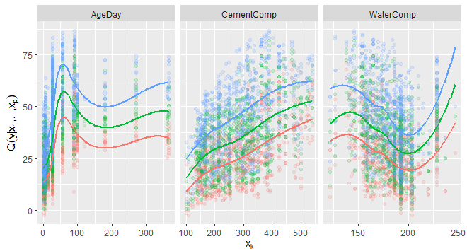
In Figure 4 the marginal effect plots based on the fitted quantiles, from the C-vine two-step model, for the three most influential predictors are given. The marginal effect of a predictor is its expected impact on the quantile estimator, where the expectation is taken over all other predictors. This is estimated using all fitted conditional quantiles and smoothed over the predictors considered.

Refer to caption — Figure 4: Marginal effect plots for the 3 most influential predictors on the concrete compressive strength for $\alpha$ values of $0.05$ (red colour), $0.5$ (green colour) and $0.95$ (blue color).

6.2 Riboflavin data set

The Riboflavin data set, available in the R package hdi, aims at quantile predictions of the log-transformed production rate of Bacillus subtilis using log-transformed expression levels of 4088 genes. To reduce the computational burden, we perform a pre-selection of the top 100 genes with the highest variance (Bühlmann and van de Geer, 2011), resulting in a subset with $p=100$ log-transformed gene expressions and $N=71$ samples. Random splitting of the subset into training set with 61 samples and evaluation set with 10 samples, is repeated for 100 times. For the C- and D-vine two-step ahead quantile regression the number of candidates is set to $k=10$ . Additionally, to further reduce the computational burden the additional variable selection from Section 4.1.1 is applied with the chosen subset containing 25% of all possible choices, where 15% are predictors having the highest partial correlation with the log-transformed Bacillus subtilis production rate and the remaining 10% are chosen randomly from the remaining predictors. Performance of competitive quantile regression models is reported in Table 7, where we see that the proposed C-vine two-step ahead quantile regression is the best performing model and outperforms both the D-vine one-step ahead quantile regression from Kraus and Czado, 2017 and the C-vine one-step ahead quantile regression to a large extent. Further, the second best performing method is the D-vine two-step ahead model which, while performing slightly worse than the C-vine two-step ahead model, also significantly outperforms both the C-vine and D-vine one-step ahead models.

Model	$\widehat{\mbox{IS}}_{0.05}$	$\widehat{\mbox{CL}}_{0.05}$	$\widehat{\mbox{CL}}_{0.5}$	$\widehat{\mbox{CL}}_{0.95}$
D-vine One-step	33.83	0.44	0.42	0.41
D-vine Two-step	30.57	0.44	0.38	0.33
C-vine One-step	34.52	0.49	0.43	0.38
C-vine Two-step	28.59	0.41	0.36	0.30

Table 7: Out-of-sample predictions

\widehat{\mbox{IS}}_{0.5}

\widehat{\mbox{CL}}_{0.05}

\widehat{\mbox{CL}}_{0.5}

\widehat{\mbox{CL}}_{0.95}

. The best performing model is highlighted in gray.

Since the predictors entering the C- and D-vine models yield a descending order of the predictors contributing to maximizing the conditional log-likelihood, the order indicates the influence of the predictors to the response variable. It is often of practical interest to know which gene expressions are of the highest importance for prediction. Since we repeat the random splitting of the subset for $R=100$ times, the importance of the gene expressions is ranked sequentially by choosing the one with the highest frequency of each element in the order excluding the gene expressions chosen in the previous steps. For instance, the most important gene expression is chosen as the one most frequently ranked first; the second most important gene is chosen as the one most frequently chosen as the second element in the order, excluding the most important gene selected in the previous step. The top ten most influential gene expressions using the C- and D-vine one- or two-step ahead models are recorded in Table 8.

Model/Position 1 2 3 4 5 6 7 8 9 10 D-vine One-step GGT YCIC MTA RPSE YVAK THIK ANSB SPOVB YVZB YQJB D-vine Two-step MTA RPSE THIK YMFE YCIC sigM PGM YACC YVQF YKPB C-vine One-step GGT YCIC MTA RPSE HIT BFMBAB PHRC YBAE PGM YHEF C-vine Two-step MTA RPSE THIK YCIC YURU PGM sigM YACC YKRM ASNB

Table 8: The 10 most influential gene expressions on the conditional quantile function, ranked based on their position in the order.

Figure 5 shows the marginal effects plots based on the fitted quantiles, from the C-vine two-step model, for the 10 most influential predictors on the log-transformed Bacillus subtilis production rate.

7 Summary and discussion

In this paper, we introduce a two-step ahead forward selection algorithm for nonparametric C- and D-vine copula based quantile regression. Inclusion of future information, obtained through considering the next tree in the two-step ahead algorithm, yields a significantly less greedy sequential selection procedure in comparison to the already existing one-step ahead algorithm for D-vine based quantile regression in Kraus and Czado, 2017. We extend the vine-based quantile regression framework to include C-vine copulas, providing an additional choice for the dependence structure. Further, for the first time, nonparametric bivariate copulas are used to construct vine copula-based quantile regression models. The nonparametric estimation overcomes the problem of possible family misspecification in the parametric estimation of bivariate copulas and allows for even more flexibility in dependence estimation. Additionally, under mild regularity conditions, the nonparametric conditional quantile estimator is shown to be consistent.
The extensive simulation study, including several different settings and data sets with different dimensions, strengths of dependence and tail dependencies, shows that the two-step ahead algorithm outperforms the one-step ahead algorithm in most scenarios. The results for the Concrete and Riboflavin data sets are especially interesting, as the C-vine two-step ahead algorithm has a significant improvement compared to the other algorithms. These findings provide strong evidence for the need of modeling the dependence structure following a C-vine copula. In addition, the two-step ahead algorithm allows controlling the computational intensity independently of the data dimensions through the number of candidate predictors and the additional variable selection discussed in Section 5. Thus, fitting vine based quantile regression models in high dimensions becomes feasible. As seen in several simulation settings, there is a significant gain by introducing additional dependence structures other then the D-vine based quantile regression. A further research area is developing similar forward selection algorithms for R-vine tree structures while optimising the conditional log-likelihood.
At each step of the vine building stage, we compare equal-sized models with the same number of variables. The conditional log-likelihood is suited for such a comparison. Other questions might come in handy, such as choosing between a C-vine, D-vine or R-vine information criteria. When maximum likelihood estimation is employed at all stages, the selection criteria by Akaike (AIC) (Akaike, 1973), the Bayesian information criterion (BIC) (Schwarz, 1978) and the focussed information criterion (FIC) (Claeskens and Hjort, 2003) might be used immediately. Ko et al., 2019 studied FIC and AIC specifically for the selection of parametric copulas. The copula information criterion in the spirit of the Akaike information criterion by Grønneberg and Hjort, 2014 can be used for selection among copula models with empirically estimated margins, while Ko and Hjort, 2019 studied such a criterion for parametric copula models. We plan a deeper investigation of the use of information criteria for nonparametrically estimated copulas and for vines in particular. Such a study is beyond the scope of this paper but could be interesting to study stopping criteria too for building vines.

Nonparametrically estimated vines are offering considerable flexibility. Their parametric counterparts, on the other hand, are enjoying simplicity. An interesting route for further research is to combine parametric and nonparametric components in the construction of the vines in an efficient way to bring the most benefit, which should be made tangible through some criterion such that guidance can be provided about which components should be modeled nonparametrically and which others are best modeled parametrically. For some types of models, such choice between a parametric and a nonparametric model has been investigated by Jullum and Hjort, 2017 via the focussed information criterion. This and alternative methods taking the effective degrees of freedom into account are worth further investigating for vine copula models.

Acknowledgments

We would like to thank the editor and the two referees for their comments, which helped to improve the manuscript. This work was supported by the Deutsche Forschungsgemeinschaft [DFG CZ 86/6-1], the Research Foundation Flanders and KU Leuven internal fund C16/20/002. The resources and services used in this work were provided by the VSC (Flemish Supercomputer Center), funded by the Research Foundation-Flanders (FWO) and the Flemish Government.

Appendix A Construction of the transformation local likelihood estimator of the copula density

Let the $N\times 2$ transformed sample matrix be

D=(S,T),

(7)

where the transformed samples $D_{n}=\big(S_{n}=\Phi^{-1}(U_{i}^{(n)}),T_{n}=\Phi^{-1}(U_{j}^{(n)})\big),n=1,\ldots,N$ , and $\Phi$ denotes the cumulative distribution function of a standard Gaussian distribution. The logarithm of the density $f_{S,T}$ of the transformed samples $(S_{n},T_{n}),n=1,\ldots,N$ is approximated locally by a bivariate polynomial expansion $P_{\bm{a}_{m}}$ of order $m$ with intercept $\tilde{a}_{m,0}$ such that the approximation is denoted by

\tilde{f}_{S,T}(\Phi^{-1}(u_{i}^{(n)}),\Phi^{-1}(u_{j}^{(n)}))=\exp\big\{\tilde{a}_{m,0}(\Phi^{-1}(u_{i}^{(n)}),\Phi^{-1}(u_{j}^{(n)}))\big\}.

The transformation local likelihood estimator is then defined as

\tilde{c}(u_{i}^{(n)},u_{j}^{(n)})=\frac{\tilde{f}_{S,T}(\Phi^{-1}(u_{i}^{(n)}),\Phi^{-1}(u_{j}^{(n)}))}{\phi(\Phi^{-1}(u_{i}^{(n)}))\phi(\Phi^{-1}(u_{j}^{(n)}))}.

(8)

To get the local polynomial approximation, we need a kernel function $K$ with 2 $\times$ 2 bandwidth matrix $\mbox{\boldmath$B$}_{N}$ . For some pair $(\check{s},\check{t})$ close to $(s,t)$ , $\log f_{ST}(\check{s},\check{t})$ is assumed to be well approximated, locally, by for instance a polynomial with $m=1$ (log-linear)

\displaystyle P_{\bm{a}_{1}}(\check{s}-s,\check{t}-t)=a_{1,0}(s,t)+a_{1,1}(s,t)(\check{s}-s)+a_{1,2}(s,t)(\check{t}-t),

or $m=2$ (log-quadratic)

	$\displaystyle P_{\bm{a}_{2}}(\check{s}-s,\check{t}-t)=a_{2,0}(s,t)+a_{2,1}(s,t)(\check{s}-s)+a_{2,2}(s,t)(\check{t}-t)$
		$\displaystyle+a_{2,3}(s,t)(\check{s}-s)^{2}+a_{2,4}(s,t)(\check{t}-t)^{2}+a_{2,5}(s,t)(\check{s}-s)(\check{t}-t).$

The coefficient vector of the polynomial expansion $P_{a_{m}}$ is denoted by $a_{m}(s,t)$ , where $a_{1}(s,t)=(a_{1,0}(s,t),\allowbreak a_{1,1}(s,t),a_{1,2}(s,t))$ for the log-linear approximation and $a_{2}(s,t)=(a_{2,0}(s,t),\ldots,a_{2,5}(s,t))$ for the log-quadratic. The estimated coefficient vector $\tilde{\mbox{\boldmath$a$}}_{m}(s,t)$ is obtained by a maximization problem in (9)

	$\displaystyle\tilde{\mbox{\boldmath$a$}}_{m}(s,t)=\arg\max_{a_{m}}\bigg\{\sum_{n=1}^{N}\mbox{\boldmath$K$}\bigg(\mbox{\boldmath$B$}_{N}^{-1/2}\begin{pmatrix}s-S_{n}\\ t-T_{n}\end{pmatrix}\bigg)P_{\bm{a}_{m}}(S_{n}-s,T_{n}-t)$						(9)
			$\displaystyle-N\Big\{\int\!\!\int_{\mathbbm{R}^{2}}\mbox{\boldmath$K$}\bigg(\mbox{\boldmath$B$}_{N}^{-1/2}\begin{pmatrix}s-\check{s}\\ t-\check{t}\end{pmatrix}\bigg)\exp\Big(P_{\bm{a}_{m}}(\check{s}-s,t-t)\Big)\mathrm{d}\check{s}\mathrm{d}\check{t}\Big\}\bigg\}.$				(9)

While it is well-known that kernel estimators suffer from the curse of dimensionality, in the vine construction only two-dimensional functions need to be estimated, this thus avoids problems with high-dimensionality.
We next explain as in Geenens et al., 2017 how a bandwidth selection is obtained. Consider the principal component decomposition for the $N\times 2$ sample matrix $D=(S,T)$ in (7), such that the $N\times 2$ matrix $(Q,R)$ follows

(Q,R)^{T}={W}D^{T},

(10)

where each row of $W$ is an eigenvector of $D^{T}D$ . We obtain an estimator of $f_{ST}$ through the density estimator of $f_{QR}$ , which can be estimated based on a diagonal bandwidth matrix $\text{diag}(h_{Q}^{2},h_{R}^{2})$ . Selecting the bandwidths $h_{Q}$ uses samples $Q_{n},n=1,\ldots,N$ as

\displaystyle h_{Q}=\arg\min_{h>0}\bigg\{\int_{-\infty}^{\infty}\Big\{\tilde{f}_{Q}^{(p)}\Big\}^{2}dq-\frac{2}{N}\sum_{n=1}^{N}\tilde{f}_{Q(-n)}^{(p)}(\hat{Q}_{n})\bigg\},

(11)

where $\tilde{f}_{Q}^{(p)}(p=1,2)$ are the local polynomial estimators for $f_{Q}$ , and $\tilde{f}_{Q(-n)}^{(p)}$ is the “leave-one-out” version of $\tilde{f}_{Q}^{(p)}$ computed by leaving out $Q_{n}$ . The procedure of selecting $h_{R}$ is similar. The bandwidth matrix for the bivariate copula density is then given by $\mbox{\boldmath$B$}_{N}=K_{N}^{(p)}{W}^{-1}\textrm{diag}(h_{Q}^{2},h_{R}^{2}){W}^{-1}$ where $K_{N}^{(p)}$ takes $N^{1/45}$ to ensure an asymptotic optimal bandwidth order for the local log-quadratic case ( $p=2$ ), see Geenens et al., 2017 for details. Selection for the k-nearest-neighbour type bandwidth is similar. The k-nearest-neighbour bandwidths denoted as $h^{\prime}_{Q}$ and $h^{\prime}_{R}$ are obtained by restricting the minimization in (11) in the interval $(0,1)$ , i.e.,

h^{\prime}_{Q}=\arg\min_{h^{\prime}_{Q}\in(0,1)}\bigg\{\int_{-\infty}^{\infty}\Big\{\tilde{f}_{Q}^{(p)}\Big\}^{2}dq-\frac{2}{N}\sum_{n=1}^{N}\tilde{f}_{Q(-n)}^{(p)}(\hat{Q}_{n})\bigg\}.

Estimating $f_{QR}$ at any $(q,r)$ is obtained by using its $k=K_{N}^{(p)}\cdot h^{\prime}_{Q}\cdot N$ nearest neighbours where $K_{N}^{(p)}$ takes $N^{-4/45}$ for $p=2$ . The R package rvinecopulib only implemented the bandwidth in (11) for the quadratic case with $p=2$ .

Appendix B Proof of Proposition 4.2

Proof.

We first show statement 1. By (3), the estimator $\hat{F}^{-1}_{Y|X_{1},\ldots,X_{p}}(\alpha|x_{1},\ldots,x_{p})=$
$\hat{F}^{-1}_{Y}\big(\hat{C}^{-1}_{V|U_{1},\ldots,U_{p}}(\alpha|\hat{u}_{1},\ldots,\hat{u}_{p})\big),$ where $\hat{u}_{j}=\hat{F}_{j}(x_{j}),j=1,\ldots,p$ denote variables on the u-scale. To avoid heavy notation, $N$ referring to the sample size will be omitted here. Following Wied and Weißbach, 2012; Silverman, 1978, to show the uniformly strong consistency of $\hat{F}^{-1}_{Y}\big(\hat{C}^{-1}_{V|U_{1},\ldots,U_{p}}(\alpha|\hat{u}_{1},\ldots,\hat{u}_{p})\big)$ , we show

\sup_{\alpha}\big|\hat{F}^{-1}_{Y}\big(\hat{C}^{-1}_{V|U_{1},\ldots,U_{p}}(\alpha|\hat{u}_{1},\ldots,\hat{u}_{p})\big)-F^{-1}_{Y}\big(C^{-1}_{V|U_{1},\ldots,U_{p}}(\alpha|u_{1},\ldots,u_{p})\big)\big|\to 0\ a.s.

To improve the readability and simplify the notation in the proof, we first introduce some shorthand notation. Define

D_{C,1}=\hat{F}^{-1}_{Y}\big(\hat{C}^{-1}_{V|U_{1},\ldots,U_{p}}(\alpha|\hat{u}_{1},\ldots,\hat{u}_{p})\big),D_{C,2}={F}^{-1}_{Y}\big(\hat{C}^{-1}_{V|U_{1},\ldots,U_{p}}(\alpha|\hat{u}_{1},\ldots,\hat{u}_{p})\big),

D_{C,3}=\hat{F}^{-1}_{Y}\big(C^{-1}_{V|U_{1},\ldots,U_{p}}(\alpha|u_{1},\ldots,u_{p})\big),D_{C,4}={F}^{-1}_{Y}\big(C^{-1}_{V|U_{1},\ldots,U_{p}}(\alpha|u_{1},\ldots,u_{p})\big),

and the two differences $D_{C}=D_{C,1}-D_{C,3}$ and $D_{F}=D_{C,3}-D_{C,4}.$
For all $\epsilon\geq 0$ ,

$\displaystyle 1$	$\displaystyle\geq$	$\displaystyle P\big(\sup_{\alpha}\big\|D_{C,1}-D_{C,4}\big\|\leq\epsilon\big)=P\big(\sup_{\alpha}\big\|D_{C,1}-D_{C,3}+D_{C,3}-D_{C,4}\big\|\leq\epsilon\big)$	(12)
	$\displaystyle=$	$\displaystyle P\big(\sup_{\alpha}\big\|D_{C}+D_{F}\big\|\leq\epsilon\big)$
	$\displaystyle\geq$	$\displaystyle P\big(\sup_{\alpha}\big\{\big\|D_{C}\big\|+\big\|D_{F}\big\|\big\}\leq\epsilon\big)\geq P\big(\sup_{\alpha}\big\|D_{C}\big\|+\sup_{\alpha}\big\|D_{F}\big\|\leq\epsilon\big)$
	$\displaystyle\geq$	$\displaystyle P\big(\big(\sup_{\alpha}\big\|D_{C}\big\|\leq\frac{3}{4}\epsilon\big)\cap\big(\sup_{\alpha}\big\|D_{F}\big\|\leq\frac{1}{4}\epsilon\big)\big)$
	$\displaystyle=$	$\displaystyle P\Big(\big(\sup_{\alpha}\big\|D_{C}\big\|\leq\frac{3}{4}\epsilon\big)\;\big\|\;\big(\sup_{\alpha}\big\|D_{F}\big\|\leq\frac{1}{4}\epsilon\big)\Big)\cdot P\big(\sup_{\alpha}\big\|D_{F}\big\|\leq\frac{1}{4}\epsilon\big).$

Denote the event $A=\sup_{\alpha}\big|D_{F}\big|\leq\frac{1}{4}\epsilon$ , $P(A)=1$ holds by the uniform strong consistency of the estimator of $F_{Y}^{-1}$ . Next,we show that the conditional probability in (12) is equal to 1.

	$\displaystyle P\big((\sup_{\alpha}\|D_{C}\|\leq\frac{3}{4}\epsilon)\;\big\|A\big)=P\big(\sup_{\alpha}\|D_{C,1}-D_{C,2}+D_{C,2}-D_{C,3}+D_{C,4}-D_{C,4}\|\leq\frac{3}{4}\epsilon\big\|A\big)$
		$\displaystyle\geq$	$\displaystyle P\big(\sup_{\alpha}\|D_{C,1}-D_{C,2}\|+\sup_{\alpha}\|D_{C,4}-D_{C,3}\|+\sup_{\alpha}\|D_{C,2}-D_{C,4}\|\leq\frac{3}{4}\epsilon\big\|A\big).$

This conditional probability is equal to 1, since the first and second supremum are less than or equal to $\frac{1}{4}\epsilon$ by conditioning on $A$ and due to the uniform consistency of $\hat{F}^{-1}_{Y}$ . The last supremum is less than or equal to $\frac{1}{4}\epsilon$ by Bartle and Joichi, 1961 on almost uniform convergence, applied to the continuous inverse distribution function $F^{-1}_{Y}$ , and taking the measurable space to be the probability space. First, $P\big(\sup_{\alpha}\big|\big(\hat{C}^{-1}_{V|U_{1},\ldots,U_{p}}(\alpha|\hat{u}_{1},\ldots,\hat{u}_{p})\big)-\big(C^{-1}_{V|U_{1},\ldots,U_{p}}(\alpha|u_{1},\ldots,u_{p})\big)\big|\leq\frac{1}{4}\epsilon\big)=1$ , which can be argued similar to (12) using the uniform consistency and continuity of the inverse of the h-functions. Next, (12) states $P(\sup_{\alpha}|D_{C,1}-D_{C,4}|\leq\epsilon)=1.$ We conclude that $\hat{F}^{-1}_{Y}\big(\hat{C}^{-1}_{V|U_{1},\ldots,U_{p}}(\alpha|\hat{u}_{1},\ldots,\hat{u}_{p})\big)$ is uniformly strong consistent.
To prove the weak consistency in 2, by Wied and Weißbach, 2012; Silverman, 1978, we only need to show $P(|D_{C,1}-D_{C,4}|\leq\epsilon)\to 1.$ Using the same technique as in (12) and a similar argument for proving statement 2 of Proposition 4.2 with Theorem 2 on convergence in measure in Bartle and Joichi, 1961, the weak consistency can be obtained.

∎

References

Akaike, (1973) Akaike, H. (1973). Information theory and an extension of the maximum likelihood principle. In Petrov, B. and Csáki, F., editors, Second International Symposium on Information Theory, pages 267–281. Akadémiai Kiadó, Budapest.
Athey et al., (2019) Athey, S., Tibshirani, J., Wager, S., et al. (2019). Generalized random forests. The Annals of Statistics, 47(2):1148–1178.
Bartle and Joichi, (1961) Bartle, R. G. and Joichi, J. T. (1961). The preservation of convergence of measurable functions under composition. Proceedings of the American Mathematical Society, 12(1):122–126.
Bartle and Sherbert, (2000) Bartle, R. G. and Sherbert, D. R. (2000). Introduction to real analysis. Wiley New York.
Bauer and Czado, (2016) Bauer, A. and Czado, C. (2016). Pair-copula bayesian networks. Journal of Computational and Graphical Statistics, 25(4):1248–1271.
Bedford and Cooke, (2002) Bedford, T. and Cooke, R. M. (2002). Vines–a new graphical model for dependent random variables. The Annals of Statistics, 30(4):1031–1068.
Belloni and Chernozhukov, (2011) Belloni, A. and Chernozhukov, V. (2011). $\ell$ 1-penalized quantile regression in high-dimensional sparse models. The Annals of Statistics, 39(1):82–130.
Bernard and Czado, (2015) Bernard, C. and Czado, C. (2015). Conditional quantiles and tail dependence. Journal of Multivariate Analysis, 138:104–126.
Breiman, (2001) Breiman, L. (2001). Random forests, machine learning 45. J. Clin. Microbiol, 2(30):199–228.
Bühlmann and van de Geer, (2011) Bühlmann, P. and van de Geer, S. (2011). Statistics for high-dimensional data: methods, theory and applications. Springer Science & Business Media.
Chang and Joe, (2019) Chang, B. and Joe, H. (2019). Prediction based on conditional distributions of vine copulas. Computational Statistics & Data Analysis, 139:45–63.
Charpentier et al., (2007) Charpentier, A., Fermanian, J.-D., and Scaillet, O. (2007). The estimation of copulas: Theory and practice. In Rank, J., editor, Copulas: from theory to application in finance, pages 35–64. London : Risk Books.
Chen et al., (2009) Chen, X., Koenker, R., and Xiao, Z. (2009). Copula-based nonlinear quantile autoregression. The Econometrics Journal, 12:S50–S67.
Cheng, (1995) Cheng, C. (1995). Uniform consistency of generalized kernel estimators of quantile density. The Annals of Statistics, 23(6):2285–2291.
Cheng, (1984) Cheng, K.-F. (1984). On almost sure representation for quantiles of the product limit estimator with applications. Sankhyā: The Indian Journal of Statistics, Series A.
Claeskens and Hjort, (2003) Claeskens, G. and Hjort, N. (2003). The focused information criterion. Journal of the American Statistical Association, 98:900–916. With discussion and a rejoinder by the authors.
Czado, (2019) Czado, C. (2019). Analyzing Dependent Data with Vine Copulas: A Practical Guide With R. Lecture Notes in Statistics. Springer International Publishing.
Dua and Graff, (2017) Dua, D. and Graff, C. (2017). UCI machine learning repository.
Durrett, (2010) Durrett, R. (2010). Probability: theory and examples. Cambridge university press.
Fenske et al., (2011) Fenske, N., Kneib, T., and Hothorn, T. (2011). Identifying risk factors for severe childhood malnutrition by boosting additive quantile regression. Journal of the American Statistical Association, 106(494):494–510.
Geenens, (2014) Geenens, G. (2014). Probit transformation for kernel density estimation on the unit interval. Journal of the American Statistical Association, 109(505):346–358.
Geenens et al., (2017) Geenens, G., Charpentier, A., and Paindaveine, D. (2017). Probit transformation for nonparametric kernel estimation of the copula density. Bernoulli, 23(3):1848–1873.
Gijbels and Matterne, (2021) Gijbels, I. and Matterne, M. (2021). Study of partial and average conditional kendall’s tau. Dependence Modeling, 9(1):82–120.
Gijbels and Mielniczuk, (1990) Gijbels, I. and Mielniczuk, J. (1990). Estimating the density of a copula function. Communications in Statistics-Theory and Methods, 19(2):445–464.
Gneiting and Raftery, (2007) Gneiting, T. and Raftery, A. E. (2007). Strictly proper scoring rules, prediction, and estimation. Journal of the American Statistical Association, 102(477):359–378.
Grønneberg and Hjort, (2014) Grønneberg, S. and Hjort, N. L. (2014). The copula information criteria. Scandinavian Journal of Statistics, 41(2):436–459.
Haff et al., (2010) Haff, I. H., Aas, K., and Frigessi, A. (2010). On the simplified pair-copula construction—simply useful or too simplistic? Journal of Multivariate Analysis, 101(5):1296–1310.
Joe, (1996) Joe, H. (1996). Families of m-variate distributions with given margins and m (m-1)/2 bivariate dependence parameters. Lecture Notes-Monograph Series, pages 120–141.
Joe, (2014) Joe, H. (2014). Dependence modeling with copulas. CRC press.
Jullum and Hjort, (2017) Jullum, M. and Hjort, N. L. (2017). Parametric or nonparametric: The FIC approach. Statistica Sinica, 27(3):951–981.
Ko and Hjort, (2019) Ko, V. and Hjort, N. L. (2019). Copula information criterion for model selection with two-stage maximum likelihood estimation. Econometrics and Statistics, 12:167 – 180.
Ko et al., (2019) Ko, V., Hjort, N. L., and Hobæk Haff, I. (2019). Focused information criteria for copulas. Scandinavian Journal of Statistics, 46(4):1117–1140.
Koenker, (2004) Koenker, R. (2004). Quantile regression for longitudinal data. Journal of Multivariate Analysis, 91(1):74–89.
(34) Koenker, R. (2005a). Quantile Regression. Cambridge University Press.
(35) Koenker, R. (2005b). Quantile Regression. Econometric Society Monographs. Cambridge University Press.
Koenker, (2011) Koenker, R. (2011). Additive models for quantile regression: Model selection and confidence bandaids. Brazilian Journal of Probability and Statistics, 25(3):239–262.
Koenker and Bassett, (1978) Koenker, R. and Bassett, G. (1978). Regression quantiles. Econometrica: journal of the Econometric Society.
Kolmogorov and Fomin, (1970) Kolmogorov, A. N. and Fomin, S. (1970). Introductory real analysis. Prentice-Hall.
Komunjer, (2013) Komunjer, I. (2013). Quantile Prediction, Chapter 17 in Handbook of Financial Econometrics, edited by Yacine Ait-Sahalia and Lars Peter Hansen. Elsevier.
Kraus and Czado, (2017) Kraus, D. and Czado, C. (2017). D-vine copula based quantile regression. Computational Statistics & Data Analysis, 110:1–18.
Li and Martin, (2017) Li, A. H. and Martin, A. (2017). Forest-type regression with general losses and robust forest. In International Conference on Machine Learning, pages 2091–2100.
Li et al., (2013) Li, Q., Lin, J., and Racine, J. S. (2013). Optimal bandwidth selection for nonparametric conditional distribution and quantile functions. Journal of Business & Economic Statistics, 31(1):57–65.
Meinshausen, (2006) Meinshausen, N. (2006). Quantile regression forests. Journal of Machine Learning Research, 7(Jun):983–999.
Nagler, (2018) Nagler, T. (2018). kdecopula: An R package for the kernel estimation of bivariate copula densities. Journal of Statistical Software, 84(7):1–22.
Nagler, (2019) Nagler, T. (2019). vinereg: D-Vine Quantile Regression. R package version 0.7.0.
Nagler et al., (2017) Nagler, T., Schellhase, C., and Czado, C. (2017). Nonparametric estimation of simplified vine copula models: comparison of methods. Dependence Modeling, 5(1):99–120.
(47) Nagler, T. and Vatter, T. (2019a). kde1d: Univariate Kernel Density Estimation. R package version 1.0.2.
(48) Nagler, T. and Vatter, T. (2019b). rvinecopulib: High Performance Algorithms for Vine Copula Modeling. R package version 0.5.1.1.0.
Noh et al., (2013) Noh, H., Ghouch, A. E., and Bouezmarni, T. (2013). Copula-based regression estimation and inference. Journal of the American Statistical Association, 108(502):676–688.
Noh et al., (2015) Noh, H., Ghouch, A. E., and Van Keilegom, I. (2015). Semiparametric conditional quantile estimation through copula-based multivariate models. Journal of Business & Economic Statistics, 33(2):167–178.
Parzen, (1962) Parzen, E. (1962). On estimation of a probability density function and mode. The Annals of Mathematical Statistics, 33(3):1065–1076.
R Core Team, (2020) R Core Team (2020). R: A Language and Environment for Statistical Computing. R Foundation for Statistical Computing, Vienna, Austria.
Ryzin, (1969) Ryzin, J. V. (1969). On strong consistency of density estimates. The Annals of Mathematical Statistics, 40(5):1765–1772.
Schwarz, (1978) Schwarz, G. (1978). Estimating the dimension of a model. The Annals of Statistics, 6(2):461–464.
Silverman, (1978) Silverman, B. W. (1978). Weak and strong uniform consistency of the kernel estimate of a density and its derivatives. The Annals of Statistics, pages 177–184.
Sklar, (1959) Sklar, M. (1959). Fonctions de repartition an dimensions et leurs marges. Publ. inst. statist. univ. Paris, 8:229–231.
Stoeber et al., (2013) Stoeber, J., Joe, H., and Czado, C. (2013). Simplified pair copula constructions—limitations and extensions. Journal of Multivariate Analysis, 119:101–118.
Tepegjozova, (2019) Tepegjozova, M. (2019). D- and c-vine quantile regression for large data sets. Masterarbeit, Technische Universität München, Garching b. München.
Van Keilegom and Veraverbeke, (1998) Van Keilegom, I. and Veraverbeke, N. (1998). Bootstrapping quantiles in a fixed design regression model with censored data. Journal of Statistical Planning and Inference, 69(1):115–131.
Wen and Wu, (2015) Wen, K. and Wu, X. (2015). An improved transformation-based kernel estimator of densities on the unit interval. Journal of the American Statistical Association, 110(510):773–783.
Wied and Weißbach, (2012) Wied, D. and Weißbach, R. (2012). Consistency of the kernel density estimator: a survey. Statistical Papers, 53(1):1–21.
Xiao and Koenker, (2009) Xiao, Z. and Koenker, R. (2009). Conditional quantile estimation for generalized autoregressive conditional heteroscedasticity models. Journal of the American Statistical Association, 104(488):1696–1712.
Yeh, (1998) Yeh, I.-C. (1998). Modeling of strength of high-performance concrete using artificial neural networks. Cement and Concrete research, 28(12):1797–1808.
Yu and Jones, (1998) Yu, K. and Jones, M. (1998). Local linear quantile regression. Journal of the American statistical Association, 93(441):228–237.
Yu and Moyeed, (2001) Yu, K. and Moyeed, R. A. (2001). Bayesian quantile regression. Statistics & Probability Letters, 54(4):437–447.
Zhu et al., (2021) Zhu, K., Kurowicka, D., and Nane, G. F. (2021). Simplified r-vine based forward regression. Computational Statistics & Data Analysis, 155:107091.