On the Minimax Spherical Designs

Weibo Fu Address: Department of Mathematics, Princeton University, Princeton, NJ 08544 Email address: wfu@math.princeton.edu , Guanyang Wang Address: Department of Statistics, Hill Center, Rutgers University, 110 Frelinghuysen Road, Piscataway, NJ 08854 Email address: guanyang.wang@rutgers.edu and Jun Yan Address: New York, NY 10036 Email address: yanjun9306@gmail.com

Date: Weibo Fu is a Ph.D. student in Department of Mathematics, Princeton University, email: wfu@math.princeton.edu. Guanyang Wang is a tenure-track assistant professor in Department of Statistics, Rutgers University, email guanyan.wang@rutgers.edu. Jun Yan has email: yanjun9306@gmail.com

Abstract.

Distributing points on a (possibly high-dimensional) sphere with minimal energy is a long-standing problem in and outside the field of mathematics. This paper considers a novel energy function that arises naturally from statistics and combinatorial optimization, and studies its theoretical properties. Our result solves both the exact optimal spherical point configurations in certain cases and the minimal energy asymptotics under general assumptions. Connections between our results and the L1-Principal Component analysis and Quasi-Monte Carlo methods are also discussed.

Key words and phrases:

minimax spherical design, minimal energy, discrepancy

1. Introduction

The problem of distributing points on a sphere with minimal energy has attracted much interest in various branches of science. Mathematically, let $p$ be a positive integer. We denote by $S^{p-1}=\left\{v\in\mathbb{R}^{p}:\|v\|=1\right\}$ the unit sphere in $\mathbb{R}^{p}$ , where $\|\cdot\|$ stands for the standard Euclidean norm. For each positive integer $n$ and a predefined energy function $E_{n,p}:(S^{p-1})^{n}\rightarrow\mathbb{R}_{\geq 0}$ , we are interested in finding the minimal energy

(1.1)

\mathcal{E}_{n,p}:=\inf_{\underline{u}\in(S^{p-1})^{n}}E_{n,p}(\underline{u})

where $\underline{u}=(u_{1},\cdots,u_{n})$ is a set of $n$ points on the unit sphere, and the corresponding optimal configurations (i.e., minimizers of the above energy function)

(1.2)

\underline{u}^{\star}:=\argmin_{\underline{u}\in(S^{p-1})^{n}}E_{n,p}(\underline{u}).

The minimal energy, unsurprisingly, depends on the energy function $E_{n,p}$ . Finding the minimal energy and the corresponding optimal configurations is a fundamental problem in extremal geometry. In the existing literature, the energy function usually takes the form $\sum\limits_{i\neq j}f(\lVert u_{i}-u_{j}\rVert)$ where $f:\mathbb{R}_{\geq 0}\rightarrow\mathbb{R}_{\geq 0}$ is a decreasing function. For example, on the unit $2$ -sphere ( $p=3$ ), the problem is known as the Smale’s seventh problem [18] when $f(x)=1/\log x$ , the Thomson problem [20] when $f(x)=1/x$ , the generalized Thomson problem or Riesz energy problem when $f(x)=1/x^{\alpha}$ for some $\alpha>0$ . Moreover, the problem is known as the Tammes problem [19] if $E_{n,p}(\underline{u}):=1/\min\lVert u_{i}-u_{j}\rVert$ . For the general $p$ -sphere, the optimal configurations are naturally connected with the well-known spherical design problem [7]. The mentioned problems are interconnected with each other, but also exciting fields independently, attracting many researchers. Taking the Thomson problem as an example, the exact optimal configurations for $S^{2}$ have only been solved for $n\leq 6$ and $n=12$ , where the case $n=5$ is solved using a sophisticated computer-assisted proof [17]. The asymptotics for the minimal energy of the generalized Thomson problem under different regimes are derived in [21] [22] [12]. We also refer the interested readers to [6], [11] [16] and the references therein for other related results.

In this paper, we consider a new energy function defined as

(1.3)

E_{n,p}(\underline{u}):=\max_{v\in S^{p-1}}\sum_{i=1}^{n}\lvert u_{i}\cdot v\rvert.

The optimal configurations which minimize (1.3) are called the minimax spherical designs as it can be written as:

(1.4)

\underline{u}^{\star}:=\argmin_{\underline{u}\in(S^{p-1})^{n}}\max_{v\in S^{p-1}}\sum_{i=1}^{n}\lvert u_{i}\cdot v\rvert.

The minimax spherical design is also related to the traditional $t$ -designs for spheres [7] and projective spaces [10]. However, their math formulations are different from our setup. In $t$ -designs, the fixed parameter $t$ stands for the degree of polynomials. A $t$ -design is a collection of points $X$ on the space of interest such that the integration over polynomials with degree no larger than $t$ matchs their averages on $X$ . In our case, the fixed parameter $n$ is the number of points on the sphere, and we look for $n$ points that minimizes the energy function as described in (1.4).

One can observe that the new energy function (1.3) is invariant under the elementwise-reflection over the origin, that is, $E_{n,p}(u_{1},\cdots,u_{n})=E_{n,p}(s_{1}u_{1},\cdots,s_{n}u_{n})$ where $(s_{1},\cdots,s_{n})$ is an arbitrary vector in $\{-1,1\}^{n}$ . Therefore, minimizing (1.3) over $n$ vectors on the $p-1$ -sphere is equivalent to minimizing (1.3) over the upper hemisphere. Therefore the minimax design can also be viewed as a way of distributing points evenly on a hemisphere, or equivalently the real projective space $\mathbb{RP}^{p-1}$ . As we will see later, this new energy functional arises naturally and has applications in combinatorial optimization, L1-Principal Component analysis (L1-PCA) and quasi-Monte Carlo. Moreover, as we will see in Lemma 2.1, finding the minimal energy (1.3) is equivalent to the combinatorial optimization problem (2.2). Formula 2.2 shares many similarities with the $L^{2}$ or spherical discrepancy [1, 5], and therefore our techniques may be of independent interest.

In this paper we consider both the exact optimal configurations under certain circumstances and the asymptotics of the minimal energy (1.3) under general assumptions. Our results are briefly summarized and discussed below:

•
We derive the exact minimax spherical deisgns and the corresponding minimal energy in the following three cases:
1. (1)
  
  Case 1: $p\geq n$ , the minimax design is the set of $n$ mutually orthogonal vectors with $\mathcal{E}_{n,p}=\sqrt{n}$ .
2. (2)
  
  Case 2: $p=2,n$ arbitrary, the minimax design is the evenly spaced points on the upper semi-circle with $\mathcal{E}_{n,2}=\sin^{-1}(\frac{\pi}{2n})$ (see also Figure 1 for illustration of the case $n=5$ ).
3. (3)
  
  Case 3: $p=3,n=4$ , the minimax design is of the so-called triangular pyramid type (see Definition 2) with $\mathcal{E}_{4,3}=\sqrt{5}$ . See also Figure 2 for illustrations.
We want to point out that Case 1 and Case 2 are essentially known (see, for example, [23]) but under different notions. Case 3 and has not been studied before which is more interesting and complicated. As side products, we characterized the local minimas of the energy function (1.3) and therefore obtained all the local minimas when $p=3,n=4$ . For the sake of completeness, we give independent proofs for all the three cases.

•

We derive the asymptotics of the minimal energy $\mathcal{E}_{n,p}$ defined in (1.1) and construct the asymptotically minimax designs. To be more precise, we prove:

(1)

When $p$ is arbitrarily fixed and $n\rightarrow\infty$ , we have

(1.5)

\frac{\Gamma(p/2)}{\sqrt{\pi}\Gamma((p+1)/2)}\leq\frac{\mathcal{E}_{n,p}}{n}\leq\frac{\Gamma(p/2)}{\sqrt{\pi}\Gamma((p+1)/2)}+C_{p}n^{-\frac{1}{p}}.

In other words, $\mathcal{E}_{n,p}\sim\frac{\Gamma(p/2)}{\sqrt{\pi}\Gamma((p+1)/2)}n$ .

(2)

When $n,p$ are two arbitrary positive integers with $n>p$ , we have $\mathcal{E}_{n,p}=\Theta(n/\sqrt{p})$ . More precisely:

(1.6) $\sqrt{\frac{2}{\pi}}\cdot\frac{n}{\sqrt{p+1}}<\mathcal{E}_{n,p}<\frac{\sqrt{5}}{2}\cdot\frac{n}{\sqrt{p}}.$

Moreover, we construct the configurations that attain the minimal energy asymptotically using the sphere’s area-regular partitions. We further conjecture the quantity $\mathcal{E}_{n,p}/n$ which represents the average energy is decreasing with $n$ when $p$ is fixed, but we do not know how to prove it.

Figure 1. The spherical design for

n=5,p=2

. The five blue vectors

\{v_{1},v_{2},\cdots,v_{5}\}

are five evenly spaced points on the semicircle, the rest five red vectors

\{v_{1}^{\prime},v_{2}^{\prime},\cdots,v_{5}^{\prime}\}

are the antipodal points of

\{v_{1},v_{2},\cdots,v_{5}\}

Figure 2. The spherical design for

n=3,p=4

. The four blue vertex of the triangular pyramid forms a spherical design. The four red vectors are the antipodal points.

Interestingly, the proof techniques for the exact minimax spherical designs and the asymptotics are quite different. Finding the exact minimax spherical designs relies on combinatorial methods. For example, the combinatorial trick given in Lemma 2.1 reduces the problem of maximizing a function (1.3) over a compact region into an issue of optimizing a function over a finite (but still exponentially large) set. Moreover, by allowing infinitesimal variations at the local minima, we are able to get extra incidence relations Lemma 2.5, and exploit them to better understand and analyze the general cases. With additional combinatorial arguments, these incidence relations help us completely settle down the problem for $n=4,p=3$ . In contrast, though the original problem itself is deterministic, the asymptotic results mostly rely on probabilistic methods. The lower bound in (1.5) is proved directly using probability arguments, and the upper bound combines probabilistic arguments with results in area-regular partitions for a unit sphere.

The rest of this paper is organized as follows. Section 2 solves the minimal energy and the corresponding minimax spherical designs for Case 1 - Case 3 mentioned above. Section 3 studies the asymptotic behaviors of the minimal energy $\mathcal{E}_{n,p}$ , and construct the asymptotically minimax designs. Section 4 discusses two applications: L1-PCA and Quasi-Monte Carlo. Several unsolved problems are discussed at the end of each section.

Acknowledgement

The authors would like to thank Persi Diaconis, Andrea Ottolini, and Xiaoming Huo for helpful comments and discussions.

2. Exact minimax designs

This section focuses on solving the minimal energy and the corresponding minimax designs in the three cases mentioned in Section 1. We start with proving Lemma 2.1 which will be useful throughout this section. Case 1 can also be viewed as an application of Lemma 2.1, and is proved in Proposition 2.2. Case 2 and Case 3 are proved in Proposition 2.4 and 2.6 separately. In particular, Case 3 is technically most complicated, and the proof relies on repeatedly using the idea and result of the key lemma – Lemma 2.5.

For a fix set of $n$ points $\underline{u}=(u_{1},\cdots,u_{n})$ on the unit $p$ -sphere $S^{p-1}$ , finding the energy $E_{n,p}(\underline{u})$ is equivalent to maxizing the function $g_{\underline{u}}(v):=\sum_{i=1}^{n}\lvert u_{i}\cdot v\rvert$ over $S^{p-1}$ . The following lemma (also proved in [2]) shows that the above problem is equivalent to a discrete combinatorial optimization problem.

Lemma 2.1.

With the energy function $E_{n,p}$ defined as in (1.3), for each $\underline{u}=(u_{1},\cdots,u_{n})\in(S^{p-1})^{n}$ , we have:

(2.1)

E_{n,p}(\underline{u})=\max_{v\in S^{p-1}}\sum_{i=1}^{n}\lvert u_{i}\cdot v\rvert=\max_{\delta\in\{-1,1\}^{n}}\lVert\sum_{i=1}^{n}\delta_{i}u_{i}\rVert.

Proof.

	$\displaystyle E_{n,p}(\underline{u})$	$\displaystyle=\max_{v\in S^{p-1}}\sum_{i=1}^{n}\lvert u_{i}\cdot v\rvert=\max_{v\in S^{p-1}}\sum_{i=1}^{n}\max_{\delta_{i}\in\{-1,1\}}u_{i}\cdot(\delta_{i}v)$
		$\displaystyle=\max_{v\in S^{p-1}}\max_{\delta\in\{-1,1\}^{n}}\big(\sum_{i=1}^{n}(\delta_{i}u_{i})\cdot v\big)$
		$\displaystyle=\max_{\delta\in\{-1,1\}^{n}}\max_{v\in S^{p-1}}\big(\sum_{i=1}^{n}(\delta_{i}u_{i})\cdot v\big)$
		$\displaystyle=\max_{\delta\in\{-1,1\}^{n}}\lVert\sum_{i=1}^{n}\delta_{i}u_{i}\rVert,$

where the last equality follows from the Cauchy-Schwarz inequality. After fixing $\delta\in\{-1,1\}^{n}$ , it is straightforward from Cauchy-Schwarz inequality that the quantity $\big(\sum_{i=1}^{n}(\delta_{i}u_{i})\cdot v\big)$ is no larger than $\lVert\sum_{i=1}^{n}\delta_{i}u_{i}\rVert\lVert v\rVert=\lVert\sum_{i=1}^{n}\delta_{i}u_{i}\rVert$ and is maximized by taking

v=\frac{\sum_{i=1}^{n}\delta_{i}u_{i}}{\lVert\sum_{i=1}^{n}\delta_{i}u_{i}\rVert}.

∎

Lemma 2.1 suggests, instead of searching for all the points on the sphere $S^{p-1}$ , it suffices to maximize the vectors’ Euclidean norm over a finite set of the vectors which are of the form $\sum_{i=1}^{n}\delta_{i}u_{i}$ . Consequently, the minimal energy can be equivalently written as:

(2.2)

\mathcal{E}_{n,p}=\min_{\begin{subarray}{c}\underline{u}\in(S^{p-1})^{n}\end{subarray}}\max_{\begin{subarray}{c}\delta\in\{-1,1\}^{n}\end{subarray}}\|\sum_{i=1}^{n}\delta_{i}u_{i}\|.

The problem for $p=1$ is trivial. For $n\leq p$ , it is easy to prove the above minimal energy (2.2) equals $\sqrt{n}$ , where the equality holds if and only if all the $u_{i}$ are orthogonal to each other.

Proposition 2.2 (Case 1: $n\leq p$ ).

For any positive integers $n,p$ , we have $\mathcal{E}_{n,p}\geq\sqrt{n}$ , where the equality holds if and only if $n\leq p$ and all the $u_{i}$ are orthogonal to each other.

Proof.

Consider the following equality

\sum_{\begin{subarray}{c}\delta\in\{\pm 1\}^{n}\end{subarray}}\|\sum_{i=1}^{n}\delta_{i}v_{i}\|^{2}=n2^{n},

which is true for every $\{v_{1},\cdots,v_{n}\}$ as we can expand the expression and cancel out all the cross-terms. We immediately have $n2^{n}\leq 2^{n}\max_{\delta\in\{\pm 1\}^{n}}\|\sum_{i=1}^{n}\delta_{i}v_{i}\|^{2}$ . Taking the mininum over $\{v_{1},\cdots,v_{n}\}$ on the RHS yields $\mathcal{E}_{n,p}\geq\sqrt{n}$ . The equality holds if and only if $\|\sum_{i=1}^{n}\delta_{i}v_{i}\|^{2}=n$ for any $\delta_{i}\in\{\pm 1\},~1\leq i\leq n$ . Therefore,

\|v_{n}+\sum_{i=1}^{n-1}\delta_{i}v_{i}\|^{2}=\|-v_{n}+\sum_{i=1}^{n-1}\delta_{i}v_{i}\|^{2}=n,

implying $v_{n}\perp\sum_{i=1}^{n-1}\delta_{i}v_{i}$ , which shows $v_{n}\perp v_{i}$ for all $1\leq i\leq n-1$ . We win by an easy induction. ∎

2.1. Case 2: $p=2$ , $n$ arbitrary

We now turn to Case 2. The minimal energy result depends on the following lemma.

Lemma 2.3.

Let $k$ be a positive integer. Fix $\theta\geq 0$ , let $A_{k}^{\theta}$ be the bounded region

A_{k}^{\theta}:=\left\{(\theta_{1},\cdots,\theta_{k})\in[0,\pi]^{k}|\sum_{i=1}^{k}\theta_{i}=\theta,~\theta_{i}+\theta_{i+1}\leq\pi,~1\leq i\leq k-1~\mathrm{and}~\theta_{k}+\theta_{1}\leq\pi\right\}.

We define a function $C$ on $A_{k}^{\theta}$

	$\displaystyle C:A_{k}^{\theta}$	$\displaystyle\to$	$\displaystyle\mathbb{R}_{\geq 0}$
	$\displaystyle\underline{\theta}=(\theta_{1},\cdots,\theta_{k})$	$\displaystyle\mapsto$	$\displaystyle\sum\limits_{i=1}^{k}\cos(\theta_{i}).$

Suppose $A_{k}^{\theta}$ is non-empty, or equivalently $\theta\leq\frac{k\pi}{2}$ , then $C$ attains its maximal value at $\underline{\theta}=(\frac{\theta}{k},\cdots,\frac{\theta}{k})$ with $C(\frac{\theta}{k},\cdots,\frac{\theta}{k})=k\cos(\frac{\theta}{k})$ . In particular, if $\theta<\frac{k\pi}{2}$ , then the only maximal value is attained at $\underline{\theta}=(\frac{\theta}{k},\cdots,\frac{\theta}{k})$ .

Proof.

For easing notations, we regard indices of $\theta$ as elements in $\mathbb{Z}/k\mathbb{Z}$ . In particular, $\theta_{k+1}=\theta_{1}$ . When $\theta=\frac{k\pi}{2}$ and $k$ is odd, the definition of $A_{k}^{\theta}$ forces $\theta_{1}=\theta_{2}=\cdots=\theta_{k}=\frac{\pi}{2}$ . When $\theta=\frac{k\pi}{2}$ and $k$ is even, it is clear that we can take $\theta_{1}=\theta_{2}=\cdots=\theta_{k}=\frac{\pi}{2}$ which attains the maximum $C(\underline{\theta})=0$ .

Now we assume $\theta<\frac{k\pi}{2}$ . Since $A_{k}^{\theta}$ is compact, function $C$ attains its maximal at some $\underline{\theta}=(\theta_{1},\cdots,\theta_{k})\in A_{k}^{\theta}$ . We claim that if $\underline{\theta}\neq(\frac{\theta}{k},\cdots,\frac{\theta}{k})$ , there must exist $\theta_{i}$ such that $\theta_{i}>\theta_{i+1}$ and $\theta_{i+1}+\theta_{i+2}<\pi$ . To see this, pick a $\theta_{i}$ such that $\theta_{i}=\max\{\theta_{1},\cdots,\theta_{k}\}$ , $\theta_{i}>\theta_{i+1}$ . If the claim is not true, then $\theta_{i+1}+\theta_{i+2}=\pi$ . $\theta_{i+2}=\pi-\theta_{i+1}\geq\theta_{i}$ , therefore $\theta_{i+2}=\max\{\theta_{1},\cdots,\theta_{k}\}=\theta_{i}$ . Now replace $\theta_{i}$ with $\theta_{i+2}$ , we get $\theta_{i+2}=\theta_{i+4}$ . Hence $\theta_{i}=\theta_{i+2p}$ for all $p\in\mathbb{Z}$ . If $k$ is odd, then all $\theta_{i}$ ’s are equal. If $k$ is even, then $\underline{\theta}=(\theta_{1},\pi-\theta_{1},\cdots,\theta_{1},\pi-\theta_{1})$ , $\theta=\frac{k\pi}{2}$ . Both are against the assumption. Therefore, the claim is proved.

After choosing the aforementioned index $i$ , we pick a small angle $\varepsilon>0$ such that $\theta_{i}-\varepsilon>\theta_{i+1}+\varepsilon$ and $(\theta_{i+1}+\varepsilon)+\theta_{i+2}<\pi$ . Consider a new vector $\underline{\theta^{\prime}}$ which has the $i$ -index $\theta_{i}-\varepsilon$ , $i+1$ -th index $\theta_{i+1}+\varepsilon$ and equals $\underline{\theta}$ elsewhere. Straghtforward calculation gives $C(\underline{\theta}^{\prime})-C(\underline{\theta})=\cos(\theta_{i}-\varepsilon)+\cos(\theta_{i+1}+\varepsilon)-\cos(\theta_{i})-\cos(\theta_{i+1})>0$ , which contradicts the maximal assumption. Therefore, the only maximal value of $C$ is attained at $(\frac{\theta}{k},\cdots,\frac{\theta}{k})$ , as desired.

∎

Now we are ready to solve the $p=2$ case. The minimax design is the evenly spaced points on the upper semi-circle or the evenly spaced points on the unit circle after adding all the antipodal points.

Proposition 2.4.

(Case 2: $p=2$ , n arbitrary)

\mathcal{E}_{n,2}=\min_{\begin{subarray}{c}v_{i}\in S^{1}\\ 1\leq i\leq n\end{subarray}}\max_{\begin{subarray}{c}\delta\in\{\pm 1\}^{n}\end{subarray}}\|\sum_{i=1}^{n}\delta_{i}v_{i}\|=\sin^{-1}(\frac{\pi}{2n}).

Under the standard identification $\mathbb{C}\simeq\mathbb{R}^{2}$ , $E_{n,2}(v_{1},\cdots,v_{n})=\mathcal{E}_{n,2}$ if and only if $\{\pm v_{1},\cdots,\pm v_{n}\}$ is obtained from a rotation (by a group element of $\mathrm{SO}_{2}(\mathbb{R})$ ) of $\{1,e^{\frac{\pi i}{n}},e^{\frac{2\pi i}{n}},\cdots,e^{(2n-1)\frac{\pi i}{n}}\}$ .

Proof.

Consider the unordered set $\{\pm v_{1},\cdots,\pm v_{n}\}\subset S^{1}$ , we reorder it such that $v_{1},v_{2},\cdots,v_{n},v_{n+1}:=-v_{1},v_{n+2}:=-v_{2},\cdots,v_{2n}:=-v_{m}$ is of the anti-clockwise order. Let $S_{l}:=\sum\limits_{i=l}^{n}v_{i}-\sum\limits_{j=1}^{l-1}v_{i}$ for $1\leq l\leq n$ and $S_{l}:=-S_{l-n}$ for $n+1\leq l\leq 2n$ . Let $S:=2\sum\limits_{l=1}^{n}\|S_{l}\|^{2}=\sum\limits_{l=1}^{2n}\|S_{l}\|^{2}$ .

For convenience, we regard all the indices in $\mathbb{Z}/2n\mathbb{Z}$ . For each $1\leq k\leq n-1$ , we use $\langle k\rangle$ to denote the cyclic group generated by $k$ in $\mathbb{Z}/2n\mathbb{Z}$ . It is known that the greatest common divisor $\mathrm{gcd}(k,2n)=\frac{2n}{|\langle k\rangle|}$ , and there are $\mathrm{gcd}(k,2n)$ cosets $C^{k}_{1},\cdots C^{k}_{\mathrm{gcd}(k,2n)}$ in $\mathbb{Z}/2n\mathbb{Z}$ for $\langle k\rangle$ . Let $S^{k}:=\sum\limits_{j=1}^{2n}v_{j}\cdot v_{j+k}=\sum\limits_{i=1}^{\mathrm{gcd}(k,2n)}\sum\limits_{j\in C^{k}_{i}}v_{j}\cdot v_{j+k}$ . Notice that $v_{j}+v_{j+n}=0$ ,

(2.3)

S^{k}+S^{n-k}=\sum\limits_{j=1}^{2n}v_{j}\cdot v_{j+k}+v_{j+k}\cdot v_{j+n}=0.

For each $1\leq k\leq\lfloor\frac{n}{2}\rfloor$ , since the angle between $v_{i}$ and $v_{i+2k}$ is at most $\pi$ , we have $\arccos(v_{i}\cdot v_{i+k})+\arccos(v_{i+k}\cdot v_{i+2k})\leq\pi$ . Moreover,

\sum\limits_{i=1}^{\mathrm{gcd}(k,2n)}\sum\limits_{j\in C^{k}_{i}}\arccos(v_{j}\cdot v_{j+k})=\sum\limits_{i=1}^{\mathrm{gcd}(k,2n)}\frac{2k\pi}{\mathrm{gcd}(k,2n)}=2k\pi.

We can therefore apply Lemma 2.3, which shows $S^{k}\geq 2n\cos(\frac{k\pi}{n})$ .

Now we calculate $S$

$\displaystyle S$	$\displaystyle=$	$\displaystyle 2n^{2}+2\sum_{k=1}^{n-1}(n-k)S^{k}$
	$\displaystyle\stackrel{{\scriptstyle(\ref{+=0})}}{{=}}$	$\displaystyle 2n^{2}+2\sum_{k=1}^{\lfloor\frac{n}{2}\rfloor}(n-2k)S^{k}$
	$\displaystyle\geq$	$\displaystyle 2n(n+2\sum_{k=1}^{\lfloor\frac{n}{2}\rfloor}(n-2k)\cos(\frac{k\pi}{n}))$
	$\displaystyle=$	$\displaystyle\frac{4n}{1-\cos(\frac{\pi}{n})}.$

This implies $\|S_{l}\|^{2}\geq\frac{2}{1-\cos(\frac{\pi}{n})}$ for some $1\leq l\leq n$ , and therefore

(2.4)

E_{n,2}(v_{1},\cdots,v_{n})^{2}=\max_{\begin{subarray}{c}\delta\in\{\pm 1\}^{n}\\ 1\leq i\leq n\end{subarray}}\|\sum_{i=1}^{n}\delta_{i}v_{i}\|^{2}\geq\frac{2}{1-\cos(\frac{\pi}{n})}=\sin^{-2}(\frac{\pi}{2n}).

Since (2.4) holds for any $v_{1},\cdots v_{n}$ , we prove $\mathcal{E}_{n,2}^{2}\geq\sin^{-2}(\frac{\pi}{2n}).$ Moreover, the equality holds if and only if the global maximum in Lemma 2.3 is attained, which means $\{\pm v_{1},\cdots,\pm v_{m}\}$ is evenly distributed on $S^{1}$ . Therefore $\{v_{1},\cdots v_{n}\}$ is a minimax design for $p=2$ if and only if $\{\pm v_{1},\cdots,\pm v_{n}\}$ is obtained from a rotation (by a group element of $\mathrm{SO}_{2}(\mathbb{R})$ ) of $\{1,e^{\frac{\pi i}{n}},e^{\frac{2\pi i}{n}},\cdots,e^{(2n-1)\frac{\pi i}{n}}\}$ . ∎

2.2. Case 3: $p=3$ , $n=4$

We now turn our attention to the $p=3,n>3$ case. It turns out that finding the global minimal of $E_{n,3}$ is quite difficult, as the function usually has more than one local minimal. Now we can only find all the local minimals and thus solve the case $p=3,n=4$ . We need a few more definitions and lemmas to study the properties of local minimas.

Consider the function

l:(S^{p-1})^{n}\to\mathbb{R}_{\geq 0},~~l(v_{1},\cdots,v_{n}):=\max_{\begin{subarray}{c}\delta\in\{-1,1\}^{n}\end{subarray}}\|\sum_{i=1}^{n}\delta_{i}v_{i}\|^{2}.

We say $l$ attains its local minimal at $\underline{v}=(v_{1},\cdots,v_{n})$ if $l(\underline{v})$ is the minimal value of $l$ in a neighborhood of $\underline{v}$ in $(S^{p-1})^{n}$ .

For each fixed $\underline{v}\in(S^{p-1})^{n}$ and each $\alpha=(\alpha_{1},\cdots,\alpha_{n})\in\{\pm 1\}^{n}$ , we define $V_{\alpha}:=\sum\limits_{i=1}^{n}\alpha_{i}v_{i}$ . We also denote by $\pm M_{\underline{v}}:=\{\beta\in\{\pm 1\}^{n}|\|V_{\beta}\|^{2}=l(\underline{v})\}$ the index set which contains all the binary antipodal combinations of $v$ that attains $l(\underline{v})$ . It is clear that $\pm M_{\underline{v}}$ is invariant under sign flips, that is, $\alpha\in\pm M_{\underline{v}}$ is equivalent to $-\alpha\in\pm M_{\underline{v}}$ . Therefore we can choose $M_{\underline{v}}\subset\pm M_{\underline{v}}$ such that $\pm M_{\underline{v}}=M_{\underline{v}}\cup-M_{\underline{v}}$ , and $M_{\underline{v}}\cap-M_{\underline{v}}=\emptyset$ , where $-M_{\underline{v}}:=\{\alpha\in\{\pm 1\}^{n}|-\alpha\in M_{\underline{v}}\}$ . The next lemma studies the behavior of the local minimals of the function $l$ .

Lemma 2.5.

Suppose $l$ attains its local minimal at $\underline{v}=(v_{1},\cdots,v_{n})$ . For each $1\leq i\leq n$ and $\alpha\in M_{\underline{v}}$ , there exist $c^{i}_{\alpha}\in\mathbb{R}$ such that the vector $(c^{i}_{\alpha})_{\alpha}\neq\vec{0}\in\mathbb{R}^{|M_{\underline{v}}|}$ , and $\sum\limits_{\alpha\in M_{\underline{v}}}c^{i}_{\alpha}V_{\alpha}\in\mathbb{R}^{p}$ is a scalar multiple of $v_{i}$ for every $1\leq i\leq n$ .

Proof.

Let $T_{i}$ be the tangent space of $v_{i}$ on $S^{p-1}$ translated to the orgin as a linear subspace of $\mathbb{R}^{p}$ (comprising by vectors orthogonal to $v_{i}$ ). We define a linear map $D$ (which can be viewed as essentially a directional derivative) from $\prod\limits_{i=1}^{n}T_{i}$ to $\mathbb{R}^{|M_{\underline{v}}|}$ as follows.

	$\displaystyle D:\prod\limits_{i=1}^{n}T_{i}$	$\displaystyle\to$	$\displaystyle\mathbb{R}^{\|M_{\underline{v}}\|}$
	$\displaystyle(t_{i})_{1\leq i\leq n}$	$\displaystyle\mapsto$	$\displaystyle(\langle V_{\alpha},\sum\limits_{j=1}^{n}\alpha_{j}t_{j}\rangle)_{\alpha\in M_{\underline{v}}}$

By the minimal assumption, we claim:

Claim 1.

The image of $D$ does not intersect with $\mathbb{R}_{<0}^{|M_{\underline{v}}|}$ , in other words, every vector in the image of $D$ must have at least one non-negative coordinate.

Assume for the claim is true, then $D$ is clearly not surjective. Since $D$ is a linear but not surjective map, there exists a nonzero vector which is orthogonal to the image of $D$ . In other words, we can find a non-zero vector $(c_{\alpha})_{\alpha}\in\mathbb{R}^{|M_{\underline{v}}|}$ such that

(2.5)

\sum_{\alpha\in M_{\underline{v}}}c_{\alpha}\langle V_{\alpha},\sum\limits_{j=1}^{n}\alpha_{j}t_{j}\rangle=0,~\mathrm{for~any~}(t_{i})_{1\leq i\leq n}\text{ with }t_{i}\in T_{i},1\leq i\leq n.

Taking $c_{\alpha}^{i}:=c_{\alpha}\alpha_{i}$ , as

0=\sum_{\alpha\in M_{\underline{v}}}c_{\alpha}\langle V_{\alpha},\sum\limits_{j=1}^{n}\alpha_{j}t_{j}\rangle=\sum\limits_{i=1}^{n}\langle\sum\limits_{\alpha\in M_{\underline{v}}}c_{\alpha}^{i}V_{\alpha},t_{i}\rangle,

we conclude that $\langle\sum\limits_{\alpha\in M_{\underline{v}}}c_{\alpha}^{i}V_{\alpha},t_{i}\rangle=0$ for any $t_{i}\in T_{i}$ , therefore the vector $\sum\limits_{\alpha\in M_{\underline{v}}}c_{\alpha}^{i}V_{\alpha}$ is orthogonal to the tanget space $T_{i}$ and is in turn a scalar multiple of $v_{i}$ , as desired.∎

We conclude Lemma 2.5 by proving Claim 1:

Proof of Claim 1.

Assume for contradiction that there exists a vector $t^{\circ}:=(t^{\circ}_{i})_{i\in\{1,2,\cdots,n\}}\in\prod\limits_{i=1}^{n}T_{i}$ such that $\langle V_{\alpha},\sum\limits_{j=1}^{n}\alpha_{j}t^{\circ}_{j}\rangle<0$ for every $\alpha\in M_{\underline{v}}$ . We may assume without loss of generality that $||t^{\circ}_{i}||\leq 1$ for all $1\leq i\leq m$ . We can then pertube each $v_{i}$ a little bit to construct a new set of vectors $\underline{\tilde{v}}$ which has a smaller value of $l$ , and therefore contradicts with the assumption that $l$ attains local minimum at $\underline{v}$ .

Let $r:=\max_{\alpha\in M_{\underline{v}}}\langle V_{\alpha},\sum\limits_{j=1}^{n}\alpha_{j}t^{\circ}_{j}\rangle<0$ and $\Delta=l(\underline{v})-\max_{\alpha\notin\pm M_{\underline{v}}}\lVert V_{\alpha}\rVert>0$ . Choose a small $\epsilon>0$ which satisfies

(2.6)

(2nl(\underline{v})+n^{2})\varepsilon+2n^{2}\varepsilon^{2}+n^{2}\varepsilon^{3}<-2r,

and

(2.7)

\epsilon<\frac{\Delta}{4n}.

Set $\underline{\tilde{v}}:=(\tilde{v}_{1},\cdots,\tilde{v}_{n})$ where $\tilde{v}_{i}:=\frac{v_{i}+\varepsilon t^{\circ}_{i}}{||v_{i}+\varepsilon t^{\circ}_{i}||}$ . For every $\alpha\in M_{\underline{v}}$ , we calculate $\lVert\sum_{i=1}^{n}\alpha_{i}\tilde{v}_{i}\rVert^{2}$ as:

	$\displaystyle\lVert\sum_{i=1}^{n}\alpha_{i}\tilde{v}_{i}\rVert^{2}=\lVert\sum_{i=1}^{n}\alpha_{i}\frac{v_{i}+\varepsilon t^{\circ}_{i}}{\lVert v_{i}+\varepsilon t^{\circ}_{i}\rVert}\rVert^{2}$	$\displaystyle=\lVert\sum_{i=1}^{n}\bigg(\alpha_{i}\big(\frac{1}{\lVert v_{i}+\varepsilon t^{\circ}_{i}\rVert}-1\big)(v_{i}+\varepsilon t_{i}^{\circ})\bigg)+V_{\alpha}+\varepsilon\sum_{i=1}^{n}\alpha_{i}t_{i}^{\circ}\rVert^{2}$
		$\displaystyle\leq\bigg(\sum_{i=1}^{n}(\lVert v_{i}+\varepsilon t_{i}^{\circ}\rVert-1)+\lVert V_{\alpha}+\varepsilon\sum_{i=1}^{n}\alpha_{i}t_{i}^{\circ}\rVert\bigg)^{2}$
		$\displaystyle\leq\bigg(n\varepsilon^{2}+\lVert V_{\alpha}+\varepsilon\sum_{i=1}^{n}\alpha_{i}t_{i}^{\circ}\rVert\bigg)^{2}$
		$\displaystyle=n^{2}\varepsilon^{4}+\lVert V_{\alpha}+\varepsilon\sum_{i=1}^{n}\alpha_{i}t_{i}^{\circ}\rVert^{2}+2n\varepsilon^{2}\lVert V_{\alpha}+\varepsilon\sum_{i=1}^{n}\alpha_{i}t_{i}^{\circ}\rVert$
		$\displaystyle\leq\lVert V_{\alpha}\rVert^{2}+n^{2}\varepsilon^{2}+2r\epsilon+n^{2}\varepsilon^{4}+2nl(\underline{v})\varepsilon^{2}+2n^{2}\varepsilon^{3}<\lVert V_{\alpha}\rVert^{2}$

where the first and second inequality are triangle inequalities and the last inequality is immediate after applying inequality 2.6. Meanwhile, for every $(\alpha_{1},\cdots,\alpha_{n})\in\{\pm 1\}^{n}$ , the norm difference between $\sum_{i=1}^{n}\alpha_{i}v_{i}$ and the perturbed vector $\sum_{i=1}^{n}\alpha_{i}\tilde{v}_{i}$ can be bounded by:

	$\displaystyle\lVert\sum_{i=1}^{n}\alpha_{i}(v_{i}-\tilde{v}_{i})\ \rVert$	$\displaystyle\leq\sum_{i=1}^{n}\lVert v_{i}-\tilde{v}_{i}\rVert=\sum_{i=1}^{n}\lVert v_{i}-(v_{i}+\varepsilon t_{i}^{\circ})+(1-\frac{1}{\sqrt{1+\varepsilon^{2}}})(v_{i}+\varepsilon t_{i}^{\circ})\rVert$
		$\displaystyle\leq\sum_{i=1}^{n}\bigg(\varepsilon+\sqrt{1+\varepsilon^{2}}-1\bigg)\leq 2n\epsilon<\frac{\Delta}{2}.$

Therefore, for every $\alpha\notin\pm M_{\underline{v}}$ we have,

\lVert\sum_{i=1}^{n}\alpha_{i}\tilde{v}_{i}\rVert<\lVert\sum_{i=1}^{n}\alpha_{i}v_{i}\rVert+\frac{\Delta}{2}\leq l(\underline{v})-\frac{\Delta}{2},

for every $\alpha\in\pm M_{\underline{v}}$ , we have,

\lVert\sum_{i=1}^{n}\alpha_{i}\tilde{v}_{i}\rVert<l(\underline{v}).

Combining the two cases above, we have $l(\underline{\tilde{v}})=\max_{\alpha\in\{\pm 1\}^{n}}\lVert\sum_{i=1}^{n}\alpha_{i}\tilde{v}_{i}\rVert<l(\underline{v})$ , which contradicts with the local minimal assumption. ∎

We single out two types of configurations when $n=3,~p=4$ .

For $\underline{v}=(v_{1},v_{2},v_{3},v_{4}),~v_{i}\in\mathbb{R}^{3}$ up to permutations of $\{\pm v_{1},\pm v_{2},\pm v_{3},\pm v_{4}\}$ and rotations of $\mathbb{R}^{3}$ (under action of $\mathrm{O}(3)$ ), we define the cube type and the triangular pyramid type as follows (see also 3 for illustrations):

Definition 1 (Cube Type).

The set of vectors $\underline{v}=(v_{1},v_{2},v_{3},v_{4})\in(S^{2})^{4}$ is defined to be of the cube type if $\{\pm v_{1},\pm v_{2},\pm v_{3},\pm v_{4}\}$ are $8$ vertices of the inscribed cube inside $S^{2}$

Definition 2 (Triangular Pyramid Type).

The set of vectors $\underline{v}=(v_{1},v_{2},v_{3},v_{4})\in(S^{2})^{4}$ is defined to be of the triangular pyramid type if $\pm v_{1}$ are north and south poles and $v_{2},v_{3},v_{4}$ are vertices of an equilateral triangle on the equator.

Figure 3. Left: Cube Type, Right: Triangular Pyramid Type. Notice that we flip the sign of

v_{3}

in the right subfigure for convention such that

v_{1}+v_{2}+v_{3}+v_{4}

attains the maximum of

\|\sum_{i=1}^{4}\delta_{i}v_{i}\|^{2}

Proposition 2.6.

Suppose $p=3,~n=4$ . If $l$ attains its local minimal at $\underline{v}=(v_{1},v_{2},v_{3},v_{4})$ where $\spn\{v_{1},\cdots,v_{4}\}=\mathbb{R}^{3}$ and $v_{i}\neq\pm v_{j}$ for any two indices $i\neq j$ , then $\underline{v}$ is either of cube type or of triangular pyramid type. If $\underline{v}$ is of cube type, $l(\underline{v})=\frac{16}{3}$ . If $\underline{v}$ is of triangular pyramid type, $l(\underline{v})=5$ . In particular, $l$ attains its global minimal at triangular pyramid type configurations, and

\min_{\begin{subarray}{c}\underline{v}\in(S^{2})^{4}\end{subarray}}\max_{\begin{subarray}{c}\delta\in\{\pm 1\}^{4}\end{subarray}}\|\sum_{i=1}^{4}\delta_{i}v_{i}\|^{2}=5.

Proof.

Firstly, straightforward calculation verifies the value of $l$ under the cube type equals $\frac{16}{3}$ , and the value of $l$ under the triangular pyramid type equals $5$ . Now we show that $\underline{v}=(v_{1},v_{2},\cdots,v_{4})$ will not attain the global minimal of function $l$ if $\dim(\spn(v_{1},v_{2},v_{3},v_{4})<3$ or $v_{i}=\pm v_{j}$ for some indices $i,j$ . Suppose $\dim(\spn(v_{1},v_{2},v_{3},v_{4})<3$ , then the problem reduces to Case 2 as discussed in Section 2.1, and we know the minimal value of $l$ equals $\sin(\pi/8)^{-2}\approx 6.828$ . Suppose $v_{i}=\pm v_{j}$ for some $i,j$ , we may assume without loss of generality that $v_{1}=v_{2}$ , then we claim the minimal of $l$ under this extra assumption ( $v_{1}=v_{2}$ ) equals $6=\lVert 2v1\lVert^{2}+\lVert v_{2}\lVert^{2}+\lVert v_{3}\lVert^{2}$ , and the minimum is attained when $v_{1},v_{3},v_{4}$ are mutually orthogonal. In other words,

\min_{\begin{subarray}{c}\underline{v}\in(S^{2})^{4}\\ v_{1}=v_{2}\end{subarray}}\max_{\begin{subarray}{c}\delta\in\{\pm 1\}^{4}\end{subarray}}\|\sum_{i=1}^{4}\delta_{i}v_{i}\|^{2}=6.

The proof is essentially the same as Proposition 2.2. Since values are larger than $5$ – the function value of $l$ under the triangular pyramid configuration, we may assume without loss of generality that $\spn\{v_{1},\cdots,v_{4}\}=\mathbb{R}^{3}$ and $v_{i}\neq v_{j}$ for any $i\neq j\in\{1,2,3,4\}$ .

Next, suppose $\underline{v}$ attains the local minimum of $l$ , we study the cardinality of the set $M_{\underline{v}}$ . We make the following claim, which will be proved at the end of this section.

Claim 2.

Suppose $\underline{v}=(v_{1},v_{2},v_{3},v_{4})$ satisfies the assumption in Proposition 2.6, then $|M_{\underline{v}}|\geq 3$ .

Given $|M_{\underline{v}}|\geq 3$ , we now discuss two possible cases for $M_{\underline{v}}$ separately. The two cases eventually correspond to the cube design and the triangular pyramid design, as we will see shortly.

•

Case 1: Every pair of elements in $M_{\underline{v}}$ are differed by exactly two indices. In other words, for any $\alpha$ and $\beta$ in $M_{\underline{v}}$ , there are exactly two indices $1\leq i_{1}\neq i_{2}\leq 4$ such that $\alpha_{i_{1}}=-\beta_{i_{1}},~\alpha_{i_{2}}=-\beta_{i_{2}}$ .
•

Case 2: The complement of Case 1. In other words, there exist $\alpha$ and $\beta$ in $M_{\underline{v}}$ such that they differ by one or three indices.

If $M_{\underline{v}}$ satisfies Case 1, we can make suitable relabelling such that

\{(1,1,1,1),~(1,1,-1,-1),~(1,-1,1,-1)\}\subset M_{\underline{v}}

and therefore

(2.8)

\|v_{1}+v_{2}+v_{3}+v_{4}\|^{2}=\|v_{1}+v_{2}-v_{3}-v_{4}\|^{2}=\|v_{1}-v_{2}+v_{3}-v_{4}\|^{2}.

Expanding 2.8 yields

(2.9)

\langle v_{1},v_{2}\rangle+\langle v_{3},v_{4}\rangle=\langle v_{1},v_{3}\rangle+\langle v_{2},v_{4}\rangle=-(\langle v_{1},v_{4}\rangle+\langle v_{2},v_{3}\rangle).

Now we further claim $|M_{\underline{v}}|=3$ in Case 1, as otherwise by the same argument we have:

(2.10)

\|v_{1}+v_{2}+v_{3}+v_{4}\|^{2}=\|v_{1}+v_{2}-v_{3}-v_{4}\|^{2}=\|v_{1}-v_{2}+v_{3}-v_{4}\|^{2}=\|v_{1}-v_{2}-v_{3}+v_{4}\|^{2}.

Expanding 2.10 and summing up the four terms cancels out all the cross-terms and gives us $\|v_{1}+v_{2}+v_{3}+v_{4}\|^{2}=4$ , which implies $\mathcal{E}_{4,3}\leq\sqrt{4}=2$ . However, by the averaging trick in the proof of Proposition 2.2, we know $\mathcal{E}_{4,3}\geq 2$ where the inequality holds if and only if the four vectors $v_{1},v_{2},v_{3},v_{4}$ are mutually orthogonal. In more details, we have an invariant

\sum_{\begin{subarray}{c}\delta\in\{\pm 1\}^{4}\end{subarray}}\|\sum_{i=1}^{4}\delta_{i}v_{i}\|^{2}=4\times 2^{4}.

If $\mathcal{E}_{4,3}=2$ , by the pigeonhole principle, $\|\sum\limits_{i=1}^{4}\delta_{i}v_{i}\|^{2}=4$ for all $\delta\in\{\pm 1\}^{4}$ , and $v_{i}\cdot v_{j}=0$ for all $i\neq j$ . This contradicts with the setting $p=3$ . Therefore $|M_{\underline{v}}|=3$ , as claimed.

For now, we define the following notation.

M_{1}:=v_{1}+v_{2}+v_{3}+v_{4},~M_{2}:=v_{1}+v_{2}-v_{3}-v_{4},~M_{3}:=v_{1}-v_{2}+v_{3}-v_{4}.

By Formula 2.5 in the proof of Lemma 2.5, there exists a vector $(x,y,z)\neq(0,0,0)$ such that

(2.11)

x\langle M_{1},t_{1}+t_{2}+t_{3}+t_{4}\rangle+y\langle M_{2},t_{1}+t_{2}-t_{3}-t_{4}\rangle+z\langle M_{3},t_{1}-t_{2}+t_{3}-t_{4}\rangle=0

for any $t_{i}$ in the tangent space of $v_{i}$ on $S^{2}$ . Expanding 2.11 and collecting terms with respect to $t_{i}$ yields

xM_{1}+yM_{2}+zM_{3}\parallel v_{1},~xM_{1}+yM_{2}-zM_{3}\parallel v_{2},~xM_{1}-yM_{2}+zM_{3}\parallel v_{3},~xM_{1}-yM_{2}-zM_{3}\parallel v_{4},

where $v\parallel w$ means that $v$ is parallel to $w$ in the usual Euclidean space.

Setting $a=x+y-z,~b=x-y+z,~c=x-y-z$ , the parallel relationship is further equivalent to

av_{2}+bv_{3}+cv_{4}\parallel v_{1},~av_{1}+cv_{3}+bv_{4}\parallel v_{2},~bv_{1}+cv_{2}+av_{4}\parallel v_{3},~cv_{1}+bv_{2}+av_{3}\parallel v_{4}.

As $\{v_{1},v_{2},v_{3},v_{4}\}$ spans the whole space $\mathbb{R}^{3}$ , there exists $(p_{1},p_{2},p_{3},p_{4})\neq(0,0,0,0)$ which is unique up to a scalar multiple such that $p_{1}v_{1}+p_{2}v_{2}+p_{3}v_{3}+p_{4}v_{4}=\vec{0}$ . Therefore by the parallel relations,

[p_{2}:p_{3}:p_{4}]=[a:b:c],~[p_{1}:p_{3}:p_{4}]=[a:c:b],

[p_{1}:p_{2}:p_{4}]=[b:c:a],~[p_{1}:p_{2}:p_{3}]=[c:b:a].

From the above relation we can derive that $[a:b:c]\in\{[1:1:1],[1:1:-1],[1:-1:1],[1:-1:-1]\}.$ By the fact that $M_{i}$ are nonzero vectors, the only possibility is that

[a:b:c]=[1:1:-1],~v_{1}-v_{2}-v_{3}+v_{4}=\vec{0}.

Combining $\|v_{1}-v_{2}-v_{3}+v_{4}\|=0$ , together with equation (2.9) and the fact that $\|v_{4}\|=1$ , one can solve the inner products of any pairs of $\{v_{1},v_{2},v_{3},v_{4}\}$ . The Gram matrix $G:=(\langle v_{i},v_{j}\rangle)_{1\leq i,j\leq 4}$ can be calculated as:

G=\begin{pmatrix}1&1/3&1/3&-1/3\\ 1/3&1&-1/3&1/3\\ 1/3&-1/3&1&1/3\\ -1/3&1/3&1/3&1\\ \end{pmatrix},

which corresponds to the cube type.

Otherwise, $M_{\underline{v}}$ satisfies case 2. Suitable relabelling allows us to assume that $(1,1,1,1),~(1,1,-1,-1),~(1,-1,-1,-1)\in M_{\underline{v}}$ . Similarly, we define

M_{1}:=v_{1}+v_{2}+v_{3}+v_{4},~M_{2}:=v_{1}+v_{2}-v_{3}-v_{4},~M_{3}:=v_{1}-v_{2}-v_{3}-v_{4}.

In contrary to Case 1, we will show $|M_{\underline{v}}|\geq 4$ in Case 2. Suppose $|M_{\underline{v}}|=3$ , similar to case 1, Lemma 2.5 guarantees the existence of a non-zero vector $(x,y,z)$ such that

x\langle M_{1},t_{1}+t_{2}+t_{3}+t_{4}\rangle+y\langle M_{2},t_{1}+t_{2}-t_{3}-t_{4}\rangle+z\langle M_{3},t_{1}-t_{2}-t_{3}-t_{4}\rangle=0,

for any $t_{i}$ in the tangent space of $v_{i}$ on $S^{2}$ . Equivalently, we have

(2.12)

xM_{1}+yM_{2}+zM_{3}\parallel v_{1},~xM_{1}+yM_{2}-zM_{3}\parallel v_{2},~xM_{1}-yM_{2}-zM_{3}\parallel v_{3},v_{4}.

By our assumption, two lines spanned by $v_{3}$ and $v_{4}$ are distinct, hence the third parallel relationship in 2.12 shows

(2.13)

xM_{1}-yM_{2}-zM_{3}=\vec{0}.

Plugging 2.13 back into the first two parallel relationship in 2.12 shows

xM_{1}\parallel v_{1},~yM_{2}\parallel v_{2}.

If $y=0$ , one deduces $M_{1}\parallel M_{3}\parallel v_{1}$ . Since $\|M_{1}\|=\|M_{3}\|$ by definition, we have

\displaystyle v_{2}+v_{3}+v_{4}=\vec{0},~\|M_{1}\|=\|M_{3}\|=1,

which is impossible. Similarly, the case $x=0$ can be ruled out. Therefore it suffices to discuss the case where both $x$ and $y$ are nonzero. Since we have

M_{1}\parallel v_{1},~M_{2}\parallel v_{2}.

Write $M_{1}=\lambda_{1}v_{1}$ and $M_{2}=\lambda_{2}v_{2}$ , we can use the relationship

(1-\lambda_{1})v_{1}+v_{2}+v_{3}+v_{4}=v_{1}+(1-\lambda_{2})v_{2}-v_{3}-v_{4}=0

to solve $\lambda_{1}=2,\lambda_{2}=2$ , therefore

v_{3}+v_{4}=v_{1}-v_{2},

and $M_{3}=0$ , which is also a contradiction. Therefore we know $|M_{\underline{v}}|\geq 4$ .

Given $|M_{\underline{v}}|\geq 4$ , we now discuss on the fourth vector in $M_{\underline{v}}$ other than
$(1,1,1,1),~(1,1,-1,-1),~(1,-1,-1,-1)\in M_{\underline{v}}$ . Firstly, if $(1,-1,1,1)\in M_{\underline{v}}$ , from

\|M_{1}\|=\|M_{2}\|=\|M_{3}\|=\|v_{1}-v_{2}+v_{3}+v_{4}\|

we have

v_{1}\perp v_{2}\perp v_{3}+v_{4}.

It can be directly checked that $\underline{v}$ is of the triangular pyramid type. Let $e_{3}=v_{1}\times v_{2}$ . Suppose $v_{3}=av_{1}+bv_{2}+xe_{3}$ , then $v_{4}=-av_{1}-bv_{2}+xe_{3}$ for $(a,b,x)\in S^{2}$ . Therefore $v_{3}-v_{4}=2(av_{1}+bv_{2})$ . We also know $\lVert M_{i}\rVert^{2}=1^{2}+1^{2}+(2x)^{2}=2+4x^{2}$ for any $i$ , by the maximal property of $M_{i}$ , we have,

\|v_{1}+v_{2}\pm 2(av_{1}+bv_{2})\|^{2}=4a^{2}+4b^{2}\pm 4(a+b)+2\leq 2+4x^{2}=2+4(1-a^{2}-b^{2})

\|v_{1}-v_{2}\pm 2(av_{1}+bv_{2})\|^{2}=4a^{2}+4b^{2}\pm 4(a-b)+2\leq 2+4x^{2}=2+4(1-a^{2}-b^{2}).

We have

\max{2(a^{2}+b^{2})\pm(a+b),2(a^{2}+b^{2})\pm(a-b)}\leq 1.

Without loss of generality, $a$ , $b\geq 0$ .

2(a^{2}+b^{2})+\sqrt{a^{2}+b^{2}}\leq 2(a^{2}+b^{2})+(a+b)\leq 1,

hence $a^{2}+b^{2}\leq\frac{1}{4}$ , therefore $l(\underline{v})^{2}=\lVert M_{i}\rVert^{2}\geq 2+4x^{2}=2+4(1-a^{2}-b^{2})\geq 2+4\times\frac{3}{4}=5$ , and the inequality attains equality when $\underline{v}$ is of the triangular pyramid type. In other words, up to reflections and index permutations, the Gram matrix $G:=(\langle v_{i},v_{j}\rangle)_{1\leq i,j\leq 4}$ is given by:

G=\begin{pmatrix}1&0&0&0\\ 0&1&1/2&-1/2\\ 0&1/2&1&1/2\\ 0&-1/2&1/2&1\end{pmatrix}.

The remaining cases can be argued using a similar but slightly more complicated way. Suppose that $(1,1,-1,-1)\notin M_{\underline{v}}$ , we know up to equivalence that either $(1,1,1,-1)$ or $(1,-1,1,-1)$ is in $M_{\underline{v}}$ . We will do the case where $(1,-1,1,-1)\in M_{\underline{v}}$ by contradiction, and the other case can be proved in the same way.

Suppose $(1,-1,1,-1)\in M_{\underline{v}}$ , we claim that $|M_{\underline{v}}|\geq 5$ . Otherwise, we can again write $M_{4}:=v_{1}-v_{2}+v_{3}-v_{4}$ . It can be shown from Lemma 2.5 that there exists $(x,y,z,w)\neq(0,0,0,0)$ such that

xM_{1}+yM_{2}+zM_{3}+wM_{4}\parallel v_{1},~xM_{1}+yM_{2}-zM_{3}-wM_{4}\parallel v_{2},

xM_{1}-yM_{2}-zM_{3}+wM_{4}\parallel v_{3},~xM_{1}-yM_{2}-zM_{3}-wM_{4}\parallel v_{4}.

Set

a=x+y-z-w,~b=x+y+z-w,~c=x-y+z+w,

d=x-y+z-w,~e=x-y-z+w,~f=x-y-z-w.

The parallel relations are then translated to

av_{2}+ev_{3}+fv_{4}\parallel v_{1},~av_{1}+dv_{3}+cv_{4}\parallel v_{2},

ev_{1}+dv_{2}+bv_{4}\parallel v_{3},~fv_{1}+cv_{2}+bv_{3}\parallel v_{4}.

Using the nondegeneracy of $\{v_{1},v_{2},v_{3},v_{4}\}$ (there exists a unique vector $(p_{1},p_{2},p_{3},p_{4})$ up to a scalar multiple such that $p_{1}v_{1}+p_{2}v_{2}+p_{3}v_{3}+p_{4}v_{4}=\vec{0}$ ), we deduce that

ab=ce=df\Rightarrow(x+y-w)^{2}=(x-y+w)^{2}=(x-y-w)^{2}

\Rightarrow(x,y,w)=(1,1,1)~\mathrm{or}~(1,0,0)~\mathrm{or}~(0,1,0)~\mathrm{or}~(0,0,1)

up to a scalar multiple. If $(x,y,w)=(1,1,1)$ , by the parallel relations, we deduce that

z=0,~v_{1}+v_{4}=v_{2}+v_{3},

which means

M_{3}=2v_{1},~|M_{3}|^{2}=4,~l(\underline{v})=4,

we have discussed in Proposition 2.2 that this is equivalent to the case that $v_{i}$ ’s are orthogonal to each other, yielding a contradiction. If $(x,y,w)=(1,0,0)$ (and similarly for the rest two cases),

M_{1}-zM_{3}=\vec{0},~M_{1}\parallel M_{3}\parallel v_{1}.

Since $\|M_{1}\|=\|M_{3}\|$ , $v_{2}+v_{3}+v_{4}=\vec{0}$ , we conclude $l(\underline{v})=\|M_{1}\|=\|M_{3}\|=1$ , which is also a contradiction.

Given $|M_{\underline{v}}|\geq 5$ , $\{(1,1,1,1),(1,1,-1,-1),(1,-1,-1,-1),(1,-1,1,-1)\}\subset M_{\underline{v}}$ , and $(1,-1,-1,1)\notin M_{\underline{v}}$ (otherwise $v_{i}$ ’s are all orthogonal to each other). In all the other cases, $M_{\underline{v}}$ contains four elements $\gamma,\delta,\sigma,\tau$ such that $\gamma_{i_{1}}=\gamma_{i_{2}},~\delta_{i_{1}}=\delta_{i_{2}},~\sigma_{i_{1}}=\sigma_{i_{2}},~\tau_{i_{1}}=\tau_{i_{2}}$ for two different indices $1\leq i_{1}\neq i_{2}\leq 4$ , reducing to the situation that $v_{1}\perp v_{2}\perp v_{3}+v_{4}$ , and as discussed before, corresponding to the triangular pyramid type. ∎

We conclude the proof of Proposition 2.6 by showing Claim 2.

Proof of Claim 2.

First, we claim $|M_{\underline{v}}|\geq 2$ . Suppose the contrary, since Lemma 2.5 shows the linear map from $\prod\limits_{i=1}^{n}T_{i}$ to $\mathbb{R}^{|M_{\underline{v}}|}=\mathbb{R}$ is not surjective, we immediately have $D$ is the zero map, a clear contradiction.

Suppose $|M_{\underline{v}}|=2$ and $M_{\underline{v}}=\{\alpha,\beta\}$ . The case where $\{V_{\alpha},V_{\beta}\}$ is linear independent has already been excluded by Lemma 2.5 as well, since it is shown that the non-zero linear combinations of $\{V_{\alpha},V_{\beta}\}$ will generates $\spn\{v_{1},v_{2},v_{3},v_{4}\}$ , which is of dimension $3$ , a contradiction.

It only remains to discuss the case where $\{V_{\alpha},V_{\beta}\}$ is linearly dependent. Since $\|V_{\alpha}\|=\|V_{\beta}\|$ , we have $V_{\alpha}=\pm V_{\beta}$ . We can assume $V_{\alpha}=V_{\beta}$ as otherwise we may simply choose $M_{\underline{v}}=\{\alpha,-\beta\}$ . Again, after suitable relabelling we can assume $V_{\alpha}=v_{1}+v_{2}+v_{3}+v_{4}$ , and $V_{\beta}$ is either $v_{1}+v_{2}+v_{3}-v_{4}$ or $v_{1}+v_{2}-v_{3}-v_{4}$ or $v_{1}-v_{2}-v_{3}-v_{4}$ . For the first case $v_{4}=0$ . For the second case $v_{3}$ , $v_{4}$ spans the same line (contradicts with the setting of Proposition 2.6). For the third case $V_{\beta}=v_{1}$ with unit length which contradicts with Proposition 2.2. All the cases are excluded and we conclude $|M_{\underline{v}}|\geq 3$ . ∎

Combining Proposition 2.2, 2.4, 2.6, the following theorem is immediate.

Theorem 2.7.

The minimal energy defined in (1.1) and the corresponding spherical minimax design can be explicitly derived in the following three cases:

•

Case 1: $p\geq n$ , the minimax design is the set of $n$ mutually orthogonal vectors with $\mathcal{E}_{n,p}=\sqrt{n}$ .
•

Case 2: $p=2,n$ , the minimax design is the evenly spaced points on the upper semi-circle with $\mathcal{E}_{n,2}=\sin^{-1}(\frac{\pi}{2n})$ ,
•

Case 3: $p=3,n=4$ , the minimax design is of the so-called triangular pyramid type (see Definition 2) with $\mathcal{E}_{3,4}=\sqrt{5}$ .

Proof.

Combining proposition 2.2, 2.4, and 2.6 and Theorem 2.7 automatically follows. ∎

Alas, we find our method very difficult to generalize to other cases such as $p=3$ and $n=5$ . It seems that finding the exact minimax spherical designs for general $n,p$ is a particularly challenging task. Instead of giving the exact results, we will study the asymptotic behaviors of $\mathcal{E}_{n,p}$ in the next section.

3. Asymptotic Results

We are interested in the asymptotic behavior of the quantity:

(3.1)

\displaystyle\mathcal{E}_{n,p}

\displaystyle:=\min_{\underline{u}\in(S^{p-1})^{n}}E_{n,p}(\underline{u})=\min_{u_{1},\cdots,u_{n}\in S^{p-1}}\max_{v\in S^{p-1}}\sum_{i=1}^{n}\lvert u_{i}\cdot v\rvert

under different regimes. We assume $n>p$ henceforth as otherwise the problem is solved in Section 2, Case 1. Before stating and proving our main results, we introduce two auxiliary lemmas. The first lemma shows some basic properties of a random variable uniformly distributed on $S^{p-1}$ .

Lemma 3.1 (Distribution of the first coordinate on the $p$ -sphere).

Let $v$ be a random variable which is uniformly distributed on the $S^{p-1}$ , then the first coordinate $v_{1}$ has the following probability density function on $[-1,1]:$

(3.2)

\displaystyle f_{v_{1}}(s)=\frac{(1-s^{2})^{\frac{p}{2}-\frac{3}{2}}}{B(\frac{p-1}{2},\frac{1}{2})},

where $B$ is the Beta function. Moreover, for any fixed $u\in S^{p-1}$ ,

(3.3)

\displaystyle\mathbb{E}_{v\sim\operatorname{Unif}(S^{p-1})}\lvert v\cdot u\rvert=\mathbb{E}_{v\sim\operatorname{Unif}(S^{p-1})}\lvert v_{1}\rvert=\frac{\Gamma(p/2)}{\sqrt{\pi}\Gamma((p+1)/2)}

Proof.

For the first part, let $Z_{1},Z_{2},\cdots,Z_{p}$ be independent and identically distributed (i.i.d.) standard normal random variables. It is well known that the following random vector:

\bigg(\frac{Z_{1}}{\sqrt{\sum_{i=1}^{p}Z_{i}^{2}}},\frac{Z_{2}}{\sqrt{\sum_{i=1}^{p}Z_{i}^{2}}}\cdots,\frac{Z_{p}}{\sqrt{\sum_{i=1}^{p}Z_{i}^{2}}}\bigg)^{\intercal}

is uniformly distributed on the sphere. Therefore,

(3.4)

\displaystyle\mathbb{P}\bigg(\bigg\lvert\frac{Z_{1}}{\sqrt{\sum_{i=1}^{p}Z_{i}^{2}}}\bigg\rvert\leq s\bigg)=\mathbb{P}\bigg(\frac{\sum_{i=2}^{p}Z_{i}^{2}}{Z_{1}^{2}}\geq\frac{1}{s^{2}}-1\bigg)=\mathbb{P}\bigg(\frac{\sum_{i=2}^{p}Z_{i}^{2}}{(p-1)Z_{1}^{2}}\geq\frac{(1/{s^{2}}-1)}{p-1}\bigg),

where the RHS of (3.4) can be expressed by the CDF of the $F_{p-1,1}$ distribution which has known density function. Taking the derivative of (3.4) with respect to $s$ and (3.2) follows.

To prove (3.3), we observe that the uniform distribution on $S^{p-1}$ is rotational invariant, therefore the quantity $\mathbb{E}_{v\sim\operatorname{Unif}(S^{p-1})}\lvert v\cdot u\rvert$ does not depend on $u$ . We may simply choose $u=e_{1}=(1,0,\cdots,0)^{\intercal}$ which proves the first equality of (3.3). The second equality of (3.3) are straightforward. ∎

Let $\sigma_{p}$ be the standard Euclidean Lebesgue measure on the unit sphere $S^{p-1}$ . Let $\{\mathcal{R}_{1},\mathcal{R}_{2},\cdots,\mathcal{R}_{n}\}$ be a disjoint collection such that $\mathcal{R}_{i}\subset S^{p-1}$ for each $i$ . The collection is called an area-regular partition if $\cup_{i}\mathcal{R}_{i}=S^{p-1}$ and $\sigma_{p}(\mathcal{R}_{i})=\frac{\sigma_{p}(S^{p-1})}{n}$ for every $i$ .

The second auxiliary lemma is about the area regular partitions of $S^{p-1}$ , see [3] [12] for proofs.

Lemma 3.2 (Area-regular partition).

For each $n,p\in\mathbb{N}$ , there exists an area-regular partition $\{\mathcal{R}_{1},\mathcal{R}_{2},\cdots,\mathcal{R}_{n}\}$ of the unit sphere $S^{p-1}$ such that:

\max_{i}\text{diam~}\mathcal{R}_{i}\leq C_{p}n^{-1/p},

where $C_{p}$ is a constant depending only on $p$ , $\text{diam~}\mathcal{R}_{i}:=\max_{x,y\in\mathcal{R}_{i}}\|x-y\|$ .

With all the lemmas in hand, now we are ready to prove the asymptotic results of $\mathcal{E}_{n,p}$ . We first consider the case that $p$ is a fixed positive integer and $n$ goes to infinity.

Theorem 3.3 (Asymptotics for $p$ fixed, $n\rightarrow\infty$ ).

With all the notations as above, we have the following:

(3.5)

\displaystyle\frac{\Gamma(p/2)}{\sqrt{\pi}\Gamma((p+1)/2)}\leq

\displaystyle\frac{\mathcal{E}_{n,p}}{n}\leq\frac{\Gamma(p/2)}{\sqrt{\pi}\Gamma((p+1)/2)}+C_{p}n^{-\frac{1}{p}}.

The above result shows $\mathcal{E}_{n,p}$ grows linearly with $n$ at the rate of $\frac{\Gamma(p/2)}{\sqrt{\pi}\Gamma((p+1)/2)}$ . The proof relies on a probabilistic argument. More precisely, we aim to show the following:

\mathcal{E}_{n,p}\approx\mathbb{E}_{v,\underline{u}}(\sum_{i=1}^{n}\lvert u_{i}\cdot v\rvert),

where $v,u_{1},\cdots,u_{n}$ are independent and identically distributed (i.i.d.) uniform random variables on $S^{p-1}$ .

Proof.

We start with proving the lower bound of (3.5), observe that for any $\underline{u}\in(S^{p-1})^{n}$ ,

E_{n,p}(\underline{u})=\max_{v\in S^{p-1}}\sum_{i=1}^{n}\lvert u_{i}\cdot v\rvert\geq\mathbb{E}_{v\sim\operatorname{Unif}(S^{p-1})}(\sum_{i=1}^{n}\lvert u_{i}\cdot v\rvert)=\sum_{i=1}^{n}\mathbb{E}_{v\sim\operatorname{Unif}(S^{p-1})}(\lvert u_{i}\cdot v\rvert).

In view of Lemma 3.1, we have:

\mathbb{E}_{v\sim\operatorname{Unif}(S^{p-1})}\lvert u_{i}\cdot v\rvert=\mathbb{E}_{v\sim\operatorname{Unif}(S^{p-1})}\lvert e_{1}\cdot v\rvert=\frac{\Gamma(p/2)}{\sqrt{\pi}\Gamma((p+1)/2)},

where $e_{1}=(1,0,\cdots,0)^{\intercal}$ . It is then clear that

E_{n,p}(\underline{u})\geq n\frac{\Gamma(p/2)}{\sqrt{\pi}\Gamma((p+1)/2)},

for any $\underline{u}$ . Taking infimum over $\underline{u}\in(S^{p-1})^{n}$ yields

\mathcal{E}_{n,p}\geq n\frac{\Gamma(p/2)}{\sqrt{\pi}\Gamma((p+1)/2)},

which proves the LHS of (3.5).

To prove the RHS of 3.5, let $\{\mathcal{R}_{1},\mathcal{R}_{2},\cdots,\mathcal{R}_{n}\}$ be the area-regular partition given by Lemma 3.2. For each $i$ , we pick an arbitrary $u_{i}\in\mathcal{R}_{i}$ . Then it is clear that

(3.6)

\displaystyle\mathcal{E}_{n,p}\leq\max_{v\in S^{p-1}}\sum_{i=1}^{n}\lvert u_{i}\cdot v\rvert.

On the other hand, for each fixed $v_{0}\in S^{p-1}$ ,

(3.7)		$\displaystyle\mathbb{E}_{w\sim\operatorname{Unif}(S^{p-1})}\lvert w\cdot v_{0}\rvert$	$\displaystyle=\frac{\int_{S^{p-1}}\|w\cdot v_{0}\|\sigma_{p}(dw)}{\sigma_{p}(S^{p-1})}=\frac{\sum_{i=1}^{n}\int_{\mathcal{R}_{i}}\|w\cdot v_{0}\|\sigma_{p}(dw)}{\sigma_{p}(S^{p-1})}$
(3.8)			$\displaystyle=\frac{\sum_{i=1}^{n}\mathbb{E}_{w\sim\operatorname{Unif}(\mathcal{R}_{i})}\lvert w\cdot v_{0}\rvert}{n}.$

For each $w\in\mathcal{R}_{i}$ , we have:

\displaystyle\bigl\lvert\lvert w\cdot v_{0}\rvert-\lvert u_{i}\cdot v_{0}\rvert\bigr\rvert\leq\lvert(w-u_{i})\cdot v_{0}\rvert\leq\text{diam~}\mathcal{R}_{i}\leq C_{p}n^{-1/p}

in view of the triangle inequality and Cauchy-Schwarz inequality. Therefore,

\displaystyle\lvert u_{i}\cdot v_{0}\rvert\leq\mathbb{E}_{w\sim\operatorname{Unif}(\mathcal{R}_{i})}\lvert w\cdot v_{0}\rvert+C_{p}n^{-1/p},

and $\sum_{i=1}^{n}\lvert u_{i}\cdot v_{0}\rvert$ can be upper bounded by

	$\displaystyle\sum_{i=1}^{n}\lvert u_{i}\cdot v_{0}\rvert$	$\displaystyle\leq\big(\sum_{i=1}^{n}\mathbb{E}_{w\sim\operatorname{Unif}(\mathcal{R}_{i})}\lvert w\cdot v_{0}\rvert\big)+C_{p}n^{(p-1)/p}$
		$\displaystyle=n\mathbb{E}_{w\sim\operatorname{Unif}(S^{p-1})}\lvert w\cdot v_{0}\rvert+C_{p}n^{(p-1)/p}$
		$\displaystyle=n\cdot\bigg(\frac{\Gamma(p/2)}{\sqrt{\pi}\Gamma((p+1)/2)}+C_{p}n^{-\frac{1}{p}}\bigg).$

The above inequality holds for every $v_{0}\in S^{p-1}$ , thus taking supremum over $v_{0}$ yields

\displaystyle\mathcal{E}_{n,p}\leq E_{n,p}(\underline{u})=\max_{v\in S^{p-1}}\sum_{i=1}^{n}\lvert u_{i}\cdot v\rvert\leq n\cdot\bigg(\frac{\Gamma(p/2)}{\sqrt{\pi}\Gamma((p+1)/2)}+C_{p}(n^{-\frac{1}{p}})\bigg),

which completes the proof of the RHS of (3.5). ∎

The above proof also gives us the construction of an asymptotically minimax design. The next corollary is immediate.

Corollary 1.

Let $p$ be fixed, and $\{\mathcal{R}_{1},\mathcal{R}_{2},\cdots,\mathcal{R}_{n}\}$ be an area-regular partition of $S^{p-1}$ given by Lemma 3.2. For each $i$ , we pick an $u_{i}\in\mathcal{R}_{i}$ uniformly. Then $\underline{u^{\star}}:=(u_{1},u_{2},\cdots,u_{n})$ is an asymptotically minimax design. In other words, $E_{n,p}(\underline{u^{\star}})\rightarrow\mathcal{E}_{n,p}$ as $n\rightarrow\infty$ .

If we allow both $n,p$ to be arbitrarily large, the next result shows $\mathcal{E}_{n,p}$ is always at the magnitude of $\Theta(\frac{n}{\sqrt{p}})$ .

Theorem 3.4.

Let $n,p$ be two arbitrary positive integers with $n>p$ ,

(3.9)

\displaystyle\sqrt{\frac{2}{\pi}}\cdot\frac{n}{\sqrt{p+1}}<\mathcal{E}_{n,p}<\frac{\sqrt{5}}{2}\cdot\frac{n}{\sqrt{p}}.

Proof.

We start with the lower bound in (3.9). Theorem 3.3 shows $\mathcal{E}_{n,p}\geq n\frac{\Gamma(p/2)}{\sqrt{\pi}\Gamma((p+1)/2)}$ for any $n,p$ . Using the Gautschi’s inequality

\displaystyle\frac{\Gamma(x+1)}{\Gamma(x+s)}<(x+1)^{1-s}\qquad\text{if}~~x>0,s\in(0,1)

with $x=\frac{p-1}{2}$ and $s=\frac{1}{2}$ , we have

\displaystyle n\frac{\Gamma(p/2)}{\sqrt{\pi}\Gamma((p+1)/2)}>\frac{n}{\sqrt{\pi}}\sqrt{\frac{2}{p+1}},

as desired.

For the upper bound, we write $n=kp+r$ with $k\in\mathbb{N}^{+}$ and $0\leq r\leq p-1$ . For every $i\in\{1,\cdots,n\}$ , we choose $u_{i}=e_{m_{i}}\in S^{p-1}$ with $m_{i}=i\mod p$ , where $e_{k}$ denotes the unit vector with all the entries zero except for a one on the $k$ -th coordinate. In view of Lemma 2.1, the energy $E_{n,p}(u_{1},\cdots,u_{n})$ can be calculated explicitly as:

\displaystyle E_{n,p}(u_{1},\cdots,u_{n})

\displaystyle=\lVert\sum_{i=1}^{n}u_{i}\rVert=\sqrt{r(k+1)^{2}+(p-r)k^{2}}=\sqrt{pk^{2}+2kr+r},

which can be upper bounded by

\displaystyle E_{n,p}(u_{1},\cdots,u_{n})

\displaystyle=\sqrt{\frac{(pk+r)^{2}+(p-r)r}{p}}\leq\sqrt{\frac{n^{2}+\frac{p^{2}}{4}}{p}}<\frac{\sqrt{5}}{2}\cdot\frac{n}{\sqrt{p}},

which concludes the proof. ∎

We conclude this section with the following conjecture.

Conjecture 1.

Let $R_{p}(n):=\frac{\mathcal{E}_{n,p}}{n}$ be the ‘average energy’ of the minimax design on $S^{p-1}$ . For each fixed $p$ , we conjecture: $R_{p}(n)$ is a non-increasing sequence with $n$ .

There are several evidences supporting Conjecture 1. Firstly, the first $p$ terms of $R_{p}(n)$ equals exactly $1$ , while its limit equals $\frac{\Gamma(p/2)}{\sqrt{\pi}\Gamma((p+1)/2)}<1$ . Secondly, it is not hard to show $R_{p}(2n)\leq R_{p}(n)$ for every $n$ as $\mathcal{E}_{2n,p}$ is upper bounded by $2\mathcal{E}_{n,p}$ (we can repeatly choose each vector in the minimax design of $\mathcal{E}_{n,p}$ twice). Lastly, all the existing non-asymptotic results in Section 2 support our conjecture. When $p=2$ , the results in Section 2.1 confirms our conjecture. When $p=3$ , we have $R_{3}(3)=\frac{\sqrt{3}}{3}>R_{3}(4)=\frac{\sqrt{5}}{4}$ .

4. Applications

4.1. L1-Principal Component analysis

Principal component analysis (PCA) is a widely-used technique in statistical analysis for dimension reduction. However, the standard L2-PCA approaches are known to suffer from outliers. Let $X$ be a data matrix with $n$ observations and $p$ features, the first principal component (PC1) of the classical L2-PCA looks for a $p$ -dimensional vector $w_{(1)}\in S^{p-1}$ which maximizes the L2 norm:

(4.1)

w_{(1)}:=\argmax_{w\in S^{p-1}}\lVert Xw\rVert_{2}=\argmax_{w\in S^{p-1}}w^{\intercal}X^{\intercal}Xw.

To increase the robustness of the PCA algorithm, one proposal is to maximize the L1 norm instead of the L2 norm, the first principal component of the L1-PCA can be similarly defined as:

(4.2)

v_{(1)}:=\argmax_{v\in S^{p-1}}\lVert Xv\rVert_{1}=\argmax_{v\in S^{p-1}}\sum_{i=1}^{n}\lvert v\cdot x_{i}\rvert,

where $x_{1},\cdots,x_{n}\in\mathbb{R}^{p}$ are the rows of the data matrix $X$ . It is clear that (4.2) is precisely the new energy function we have defined in 1.3. L1-PCA is often prefered than L2-PCA when the dataset has outliers or corrupted observations. Applications include image reconstruction [13], robust subspace factorization [8], regression analysis [15] and so on. Although immense progresses have been made in the study of L1-PCA methods, most of the existing results focus on proposing efficient and accurate algorithms for solving (4.2), see [15] [13] [14] for examples. Our results are directly applicable to study the behavior of L1-PCA methods in the worst-case scenario. For example, suppose we have normalized all the observations such that $x_{i}\in S^{p-1}$ for every $i$ , then Theorem 3.3 and 3.4 imply the following result directly.

Proposition 4.1.

Let $X=[x_{1}^{\intercal},x_{2}^{\intercal},\cdots,x_{n}^{\intercal}]^{\intercal}\in\mathbb{R}^{n\times p}$ be a normalized data matrix, then when $p$ is fixed and $n\rightarrow\infty$ , we have

(4.3)

\frac{\Gamma(p/2)}{\sqrt{\pi}\Gamma((p+1)/2)}\leq\frac{\min\limits_{\{x_{1},\cdots,x_{n}\}\in(S^{p-1})^{n}}\max\limits_{v\in S^{p-1}}\lVert Xv\rVert_{1}}{n}\leq\frac{\Gamma(p/2)}{\sqrt{\pi}\Gamma((p+1)/2)}+C_{p}n^{-\frac{1}{p}}.

For arbitrary positive integers $n,p>0$ , we have

(4.4)

\sqrt{\frac{2}{\pi(p+1)}}\leq\frac{\min\limits_{\{x_{1},\cdots,x_{n}\}\in(S^{p-1})^{n}}\max\limits_{v\in S^{p-1}}\lVert Xv\rVert_{1}}{n}\leq\sqrt{\frac{5}{4p}}.

The quantity $\frac{\max\limits_{v\in S^{p-1}}\lVert Xv\rVert_{1}}{n}\in[0,1]$ has natural statistical interpretations. It can be viewed as a measure for the proportion of the normalized data matrix $X$ explained by the first principal component, similar to the concept ‘Proportion of Variance Explained’ (PVE) in L2-PCA. In one extreme case (best case) where all the vectors lie on the same line, it is clear that the first principal component equals $x_{1}$ up to a sign flip. In this case we also have the ratio $\frac{\max\limits_{v\in S^{p-1}}\lVert Xv\rVert_{1}}{n}$ equals $1$ . Proposition (4.1) shows, under the worst-case scenario, the first principal component of L1-PCA can still explain $\Theta(\frac{1}{\sqrt{p}})$ of the original data. A natural follow-up problem is to consider the proportion of the original data explained by the next few principal components or ask for the number of principal components that contain a prefixed proportion of the data. We hope to answer these questions in our future works.

4.2. Quasi-Monte Carlo for surface integrals on the unit sphere

Numerical integration is an important problem in many scientific areas. Given a bounded Riemannian manifold $M\subset\mathbb{R}^{p}$ and an integration $I(f):=\int_{M}f(x)\sigma(dM)$ of interest, the standard Monte Carlo method samples independent and uniformly distributed points $x_{1},\cdots,x_{n}$ on $M$ , and estimate the integration by $\hat{I}(f):=\frac{\sum\limits_{i=1}^{n}f(x_{i})}{n}$ . By the Law of Large Numbers (LLN) and the Central Limit Theorem (CLT), the expected error of the Monte Carlo approximation is in the order of $O(n^{-1/2})$ .

When $M$ is taken to be the unit sphere $S^{p-1}$ , the spherical Quasi-Monte Carlo (QMC) seeks for $n$ points $\{u_{1},\cdots,u_{n}\}$ on the unit sphere such that the error between the empirical average of $f(u_{i})$ converges to $I(f)$ at a faster rate than the baseline $O(n^{-1/2})$ . It turns out that QMC designs are closely connected with the minimax spherical designs. Let $(u_{1},u_{2},\cdots,u_{n})$ be the asymptotically minimax spherical design selected according to Corollary 1. Then the following result from [4] shows $(u_{1},\cdots,u_{n})$ are better than the Monte Carlo method under certain smoothness assumptions.

Theorem 4.2 (Theorem 24 in [4], reformulated).

For fixed $n,p$ , let $(u_{1},\cdots,u_{n})\in(S^{p-1})^{n}$ be a set of points chosen as above. Let $\mathbb{H}^{s}(S^{p-1})$ be the Sobolev space with smoothness parameter $s$ of functions in $L^{2}(S^{p-1})$ (see [9] Chapter 5 for a detailed definition). Then the following holds for $s\in(\frac{p}{2},\frac{p}{2}+1)$ :

(4.5)

\frac{\beta^{\prime}}{n^{s/p}}\leq\sqrt{\mathbb{E}\bigg(\sup_{f\in\mathbb{H}^{s}(S^{p-1})}\big(\frac{\sum_{i=1}^{n}f(u_{i})}{n}-I(f)\big)^{2}\bigg)}\leq\frac{\beta}{n^{s/p}}

where $\beta$ and $\beta^{\prime}$ are two positive constants depending on the $\mathbb{H}^{s}(S^{p-1})$ norm but not on $n$ .

In addition to the theoretical results that consider the worst-case scenario, we also provide numerical evidence showing the QMC designs can be significantly more accurate than the Monte Carlo methods.

Example 1 (QMC design for on the unit sphere $S^{2}$ ).

The asymptotically minimax spherical design can be efficiently implemented on $S^{2}$ . For simplicity, we assume $n=(k+1)^{2}$ for some positive integer $k$ . We can evenly partition both the $z$ -axis and the longitudes into $k$ pieces. Then the sphere are naturally partitioned into $(k+1)^{2}$ pieces by the $k^{2}$ intersections. It can be directly verified that each piece has the same area, and each piece has diameter less than $4\pi n^{-\frac{1}{2}}$ . See also Figure 4 for illustrations. Therefore, by randomly choosing points on each piece, we get an asymptotically minimax spherical design of $S^{2}$ .

Figure 4. An area-regular partition of

S^{2}

Here consider three functions, $f_{1}(\vec{x})=x_{1}^{2}$ , $f_{2}(\vec{x})=1/\lVert\vec{x}-(1,1,1)\rVert$ , and $f_{3}(\vec{x})=\exp(x_{1}-x_{2})$ . The spherical surface integrals of each function can be evaluated analytically as below:

		$\displaystyle\int_{S^{2}}f_{1}(x)\sigma(dx)=\frac{4\pi^{2}}{3},$
		$\displaystyle\int_{S^{2}}f_{2}(x)\sigma(dx)=\frac{4\pi^{2}}{\sqrt{3}},$
		$\displaystyle\int_{S^{2}}f_{3}(x)\sigma(dx)=2^{\frac{3}{2}}\pi\sinh(\sqrt{2}).$

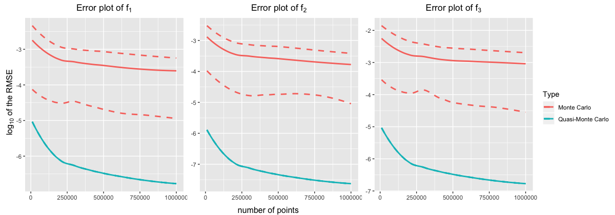
Therefore, we estimate each integral using both the Monte Carlo and the QMC methods and compare their performances. We choose $n\in[10^{4},10^{6}]$ , and implement both the Monte Carlo method and the Quasi-Monte Carlo method, each is repeated $50$ times for every fixed $n$ . The Root Mean Square Error (RMSE) of both methods are plotted below.

Refer to caption — Figure 5. Error plots of the Monte Carlo and the Quasi-Monte Carlo method for estimating the integral of $f_{1},f_{2},f_{3}$ on $S^{2}$ . The horizontal axis stands for the number of points used for estimation. The vertical axis stands for the logarithm of the root mean square error under base $10$ . Red and green solid lines correspond to the Monte Carlo and Quasi-Monte Carlo method, respectively. Red dotted lines are the $90\%$ confidence intervals of the Monte Carlo estimations based on $50$ independently repeated experiments.

Figure 5 suggests two important advantages of the QMC method, in contrast to the Monte Carlo method. Firstly, for all three test functions, QMC method offers several orders of magnitude better accuracy than the Monte Carlo method. Secondly, QMC method converges to ground truth at an order of magnitude faster than the Monte Carlo method. For all three test functions, when $n$ is increasing from $n_{1}=10^{4}$ to $n_{2}=100n_{1}=10^{6}$ , the error of the QMC method decreases to $\sim 1\%$ of the original, while the error using the Monte Carlo method only decreases to $\sim 10\%$ of the original.

Both theoretical and empirical studies have shown promising results of the QMC method, but many challenges remain. Computationally, it is unknown to us how to design efficient and implementable QMC designs when $p\gg 3$ . Mathematically, Theorem 4.2 concerns the convergence rate of a special asymptotically spherical minimax design. We do not know whether the exact spherical minimax design can achieve better convergence bounds than (4.5) or not.

References

[1] Noga Alon and Joel H Spencer, The probabilistic method, John Wiley & Sons, 2016.
[2] S Borodachov, D Hardin, and E Saff, Asymptotics for discrete weighted minimal riesz energy problems on rectifiable sets, Transactions of the American Mathematical Society 360 (2008), no. 3, 1559–1580.
[3] J Bourgain and J Lindenstrauss, Distribution of points on spheres and approximation by zonotopes, Israel Journal of Mathematics 64 (1988), no. 1, 25–31.
[4] Johann Brauchart, E Saff, I Sloan, and R Womersley, QMC designs: optimal order quasi Monte Carlo integration schemes on the sphere, Mathematics of computation 83 (2014), no. 290, 2821–2851.
[5] Bernard Chazelle, The discrepancy method: randomness and complexity, Cambridge University Press, 2001.
[6] Henry Cohn and Abhinav Kumar, Universally optimal distribution of points on spheres, Journal of the American Mathematical Society 20 (2007), no. 1, 99–148.
[7] Philippe Delsarte, Jean-Marie Goethals, and Johan Jacob Seidel, Spherical codes and designs, Geometry and Combinatorics, Elsevier, 1991, pp. 68–93.
[8] Chris Ding, Ding Zhou, Xiaofeng He, and Hongyuan Zha, R1-PCA: rotational invariant L1-norm principal component analysis for robust subspace factorization, Proceedings of the 23rd International Conference on Machine learning, 2006, pp. 281–288.
[9] Lawrence C. Evans, Partial Differential Equations (Graduate Studies in Mathematics, V. 19) GSM/19, American Mathematical Society, June 1998.
[10] Stuart G Hoggar, t-Designs in projective spaces, European Journal of Combinatorics 3 (1982), no. 3, 233–254.
[11] Ali Katanforoush and Mehrdad Shahshahani, Distributing points on the sphere, I, Experimental Mathematics 12 (2003), no. 2, 199–209.
[12] Arno Kuijlaars and E Saff, Asymptotics for minimal discrete energy on the sphere, Transactions of the American Mathematical Society 350 (1998), no. 2, 523–538.
[13] Nojun Kwak, Principal component analysis based on L1-norm maximization, IEEE transactions on pattern analysis and machine intelligence 30 (2008), no. 9, 1672–1680.
[14] Panos P Markopoulos, Sandipan Kundu, Shubham Chamadia, and Dimitris A Pados, Efficient L1-norm principal-component analysis via bit flipping, IEEE Transactions on Signal Processing 65 (2017), no. 16, 4252–4264.
[15] Michael McCoy and Joel A Tropp, Two proposals for robust PCA using semidefinite programming, Electronic Journal of Statistics 5 (2011), 1123–1160.
[16] Edward B Saff and Amo BJ Kuijlaars, Distributing many points on a sphere, The mathematical intelligencer 19 (1997), no. 1, 5–11.
[17] Richard Evan Schwartz, The five-electron case of Thomson’s problem, Experimental Mathematics 22 (2013), no. 2, 157–186.
[18] Steve Smale, Mathematical problems for the next century, The mathematical intelligencer 20 (1998), no. 2, 7–15.
[19] Pieter Merkus Lambertus Tammes, On the origin of number and arrangement of the places of exit on the surface of pollen-grains, Recueil des travaux botaniques néerlandais 27 (1930), no. 1, 1–84.
[20] Joseph John Thomson, XXIV. on the structure of the atom: an investigation of the stability and periods of oscillation of a number of corpuscles arranged at equal intervals around the circumference of a circle; with application of the results to the theory of atomic structure, The London, Edinburgh, and Dublin Philosophical Magazine and Journal of Science 7 (1904), no. 39, 237–265.
[21] Gerold Wagner, On means of distances on the surface of a sphere (lower bounds), Pacific Journal of Mathematics 144 (1990), no. 2, 389–398.
[22] by same author, On means of distances on the surface of a sphere. ii.(upper bounds), Pacific Journal of Mathematics 154 (1992), no. 2, 381–396.
[23] Chuanping Yu and Xiaoming Huo, Optimal projections in the distance-based statistical methods, Statistical Modeling in Biomedical Research, Springer, 2020, pp. 263–308.

On the Minimax Spherical Designs

Abstract.

Key words and phrases:

1. Introduction

Acknowledgement

2. Exact minimax designs

Lemma 2.1.

Proof.

Proposition 2.2 (Case 1: n≤pn\leq p).

Proof.

2.1. Case 2: p=2p=2, nn arbitrary

Lemma 2.3.

Proof.

Proposition 2.4.

Proof.

2.2. Case 3: p=3p=3, n=4n=4

Lemma 2.5.

Proof.

Claim 1.

Proof of Claim 1.

Definition 1 (Cube Type).

Definition 2 (Triangular Pyramid Type).

Proposition 2.6.

Proof.

Claim 2.

Proof of Claim 2.

Theorem 2.7.

Proof.

3. Asymptotic Results

Lemma 3.1 (Distribution of the first coordinate on the pp-sphere).

Proof.

Lemma 3.2 (Area-regular partition).

Theorem 3.3 (Asymptotics for pp fixed, n→∞n\rightarrow\infty).

Proof.

Corollary 1.

Theorem 3.4.

Proof.

Conjecture 1.

4. Applications

4.1. L1-Principal Component analysis

Proposition 4.1.

4.2. Quasi-Monte Carlo for surface integrals on the unit sphere

Theorem 4.2 (Theorem 24 in [4], reformulated).

Example 1 (QMC design for on the unit sphere S2S^{2}).

References

Proposition 2.2 (Case 1: $n\leq p$ ).

2.1. Case 2: $p=2$ , $n$ arbitrary

2.2. Case 3: $p=3$ , $n=4$

Lemma 3.1 (Distribution of the first coordinate on the $p$ -sphere).

Theorem 3.3 (Asymptotics for $p$ fixed, $n\rightarrow\infty$ ).

Example 1 (QMC design for on the unit sphere $S^{2}$ ).