regularization for convolutional kernel tensors to avoid unstable gradient problem in convolutional neural networks

As we know, each convolution arithmetic corresponds to a linear structured transformation matrix. We use $vec(X)$ to denote the vectorization of $X$. If $X$ is a matrix, $vec(X)$ is the column vector got by stacking the columns of $X$ on top of one another. If $X$ is a tensor, $vec(X)$ is the column vector got by stacking the columns of the flattening of $X$ along the first index (see [5] for more on flattening of a tensor). We use $*$ to denote the convolution arithmetic in deep learning. Given a kernel $K$, the output $Y=K*X$ can be reshaped through

where $M$ is the linear transformation matrix.

When training the deep neural networks, gradient exploding and vanishing are fundamental obstacles. It’s helpful to make the largest singular value of $M$ be smaller for controlling exploding gradients and it’s helpful to make the smallest singular value of $M$ be larger for controlling vanishing gradients. In this paper we will give three regularization terms about convolutional kernel $K$ to change the singular values of $M$ and show how to carry out gradient type methods for them.

When we refer to convolution in deep learning, there is no flip operation and only element-wise multiplication and addition are performed. Besides, in the field of deep learning, depending on different strides and padding patterns, there are many different forms of convolution arithmetic[4]. Without losing generality, in this paper we will adopt the same convolution with unit strides. We use $\ulcorner\cdot\urcorner$ is to round a number to the nearest integer greater than or equal to that number. If a convolutional kernel is a matrix $K\in\mathbb{R}^{k\times k}$ and the input is a matrix $X\in\mathbb{R}^{N\times N}$, each entry of the output $Y\in\mathbb{R}^{N\times N}$ is produced by

where $m=\ulcorner k/2\urcorner$, , and $X_{i,j}=0$ if $i\leq 0$ or $i>N$, or $j\leq 0$ or $j>N$.

In convolutional neural networks, usually there are multi-channels and a convolutional kernel is represented by a 4 dimensional tensor. If a convolutional kernel is a 4 dimensional tensor $K\in\mathbb{R}^{k\times k\times g\times h}$ and the input is 3 dimensional tensor $X\in\mathbb{R}^{N\times N\times g}$, each entry of the output $Y\in\mathbb{R}^{N\times N\times h}$ is produced by

where $m=\ulcorner k/2\urcorner$ and $X_{i,j,d}=0$ if $i\leq 0$ or $i>N$, or $j\leq 0$ or $j>N$.

In the community of deep learning, there have been papers devoted to enforcing the orthogonality or spectral norm regularization on the weights of a neural network [1, 3, 12, 19]. The difference between our paper and papers including [1, 3, 12, 19] and the references therein is about how to handle convolutions. They enforce the constraint directly on the $h\times(gkk)$ matrix reshaped from the kernel $K\in\mathbb{R}^{k\times k\times g\times h}$, while we enforce the the constraint on the transformation matrix $M$ corresponding to the convolution kernel $K$. In [13], the authors project a convolutional layer onto the set of layers obeying a bound on the operator norm of the layer and use numerical results to show this is an effective regularizer. A drawback of the method in [13] is that projection can prevent the singular values of the transformation matrix being large but can’t avoid the singular values to be too small.

In [7, 8, 17], regularization methods are proposed to let the corresponding transformation matrices be orthogonal, where the approach is to minimize the norm of $M^{T}M-I$. In this paper we propose new regularization methods for the convolutional kernel tensor $K$, which can reduce the largest singular value and increase the smallest singular value of $M$ independently or simultaneously depending on the need in the training process.

The rest of the paper is organized as follows. As we have mentioned, the input channels and the output channels maybe more than one so the kernel is usually represented by a tensor $K\in\mathbb{R}^{k\times k\times g\times h}$. In Section 2, we propose the penalty functions and calculate the partial derivatives for the case that the kernel $K$ is a $k\times k$ matrix. In Section 3, we propose the penalty functions and calculate the partial derivatives for the case that $K$ is a $k\times k\times g\times h$ tensor. In Section 4, we present numerical results to show the method is feasible and effective. In Section 5, we will give some conclusions and discuss some work that may be done in the future.

When the numbers of input channels and the output channels are both $1$, the convolutional kernel are a $k\times k$ matrix. Assuming the data matrix is $N\times N$, we use a $3\times 3$ matrix as a convolution kernel to show the associated structured transformation matrix. Let $K$ be the convolutional kernel,

Then the transformation matrix $M$ such that $vec(Y)=Mvec(X)$ for $Y=K*X$ is

where

In this case, the transformation matrix $M$ corresponding to the convolutional kernel $K$ is a $N^{2}\times N^{2}$ doubly block banded Toeplitz matrix, i.e., a block banded Toeplitz matrix with its blocks are banded Toeplitz matrices. For the details about Toeplitz matrices, please see references [2, 10]. We will let $n=N^{2}$ and use $\mathcal{T}$ to denote the set of all matrices like $M$ in (2), i.e., doubly block banded Toeplitz matrices with the fixed bandth.

For a matrix $M\in\mathcal{T}$, The value of $K_{p,q}$ will appear in different $(i,j)$ indexes. We use $\Omega$ to denote this index set, to which each $(i,j)$ index corresponding to $K_{p,q}$ belongs. That is to say, we have $m_{ij}=K_{p,q}$ for each $(i,j)\in\Omega$ and $m_{ij}\neq K_{p,q}$ for each $(i,j)$ that doesn’t satisfy $(i,j)\in\Omega$.

In this section we consider the case of multi-channel convolution. First we show the transformation matrix corresponding to multi-channel convolution. At each convolutional layer, we have convolution kernel $K\in\mathbb{R}^{k\times k\times g\times h}$ and the input $X\in\mathbb{R}^{N\times N\times g}$; element $X_{i,j,d}$ is the value of the input unit within channel $d$ at row $i$ and column $j$. Each entry of the output $Y\in\mathbb{R}^{N\times N\times h}$ is produced by

where $X_{i,j,d}=0$ if $i\leq 0$ or $i>N$, or $j\leq 0$ or $j>N$. By inspection, $vec(Y)=Mvec(X)$, where $M$ is as follows

and each $M_{(c)(d)}\in\mathcal{T}$, i.e., $M_{(c)(d)}$ is a $N^{2}\times N^{2}$ doubly block banded Toeplitz matrix corresponding to the portion $K_{:,:,d,c}$ of $K$ that concerns the effect of the $d$-th input channel on the $c$-th output channel.

Similar as the proof in Section 2, we have the following theorem.

Then the gradient descent algorithm for the penalty function $\|M\|_{F}^{2}$ can be devised, where the number of channels maybe more than one.

We present the detailed gradient descent algorithm for the three different penalty functions, where in Algorithm3.3, $min(g,h)$ denotes the smaller one of $g$ and $h$.

The numerical tests were performed on a laptop (3.0 Ghz and 16G Memory) with MATLAB R2016b. We use $M$ to denote the transformation matrix corresponding to the convolutional kernel. The largest singular value and smallest singular value of $M$ (denoted as “$\sigma_{max}(M)$ and $\sigma_{min}(M)$), the iteration steps (denoted as “iter”) are demonstrated to show the effectiveness of our method. Numerical experiments are implemented on extensive test problems. In this paper we present the numerical results for some random generated multi-channel convolution kernels, where $K$ is generated by the following command

rand(’state’,1);
$K=rand(k,k,g,h);$

We consider kernels of different sizes with $3\times 3$ filters, namely $K\in\mathbb{R}^{3\times 3\times g\times h}$ for various values of $g,h$. For each kernel, we use $20\times 20\times g$ as the size of input data matrix. We then minimize the three different penalty functions using Algorithm 3.1, 3.2 and 3.3 respectively. We show the effects of changing the singular values of $M$. We present in Figures the results for $3\times 3\times 3\times 1$ and $3\times 3\times 1\times 3$ kernels. In the figures 4.1 and 4.3, we show the convergence of $\sigma_{max}(M)$ on the left axis scale and $\sigma_{min}(M)$ on the right axis scale.

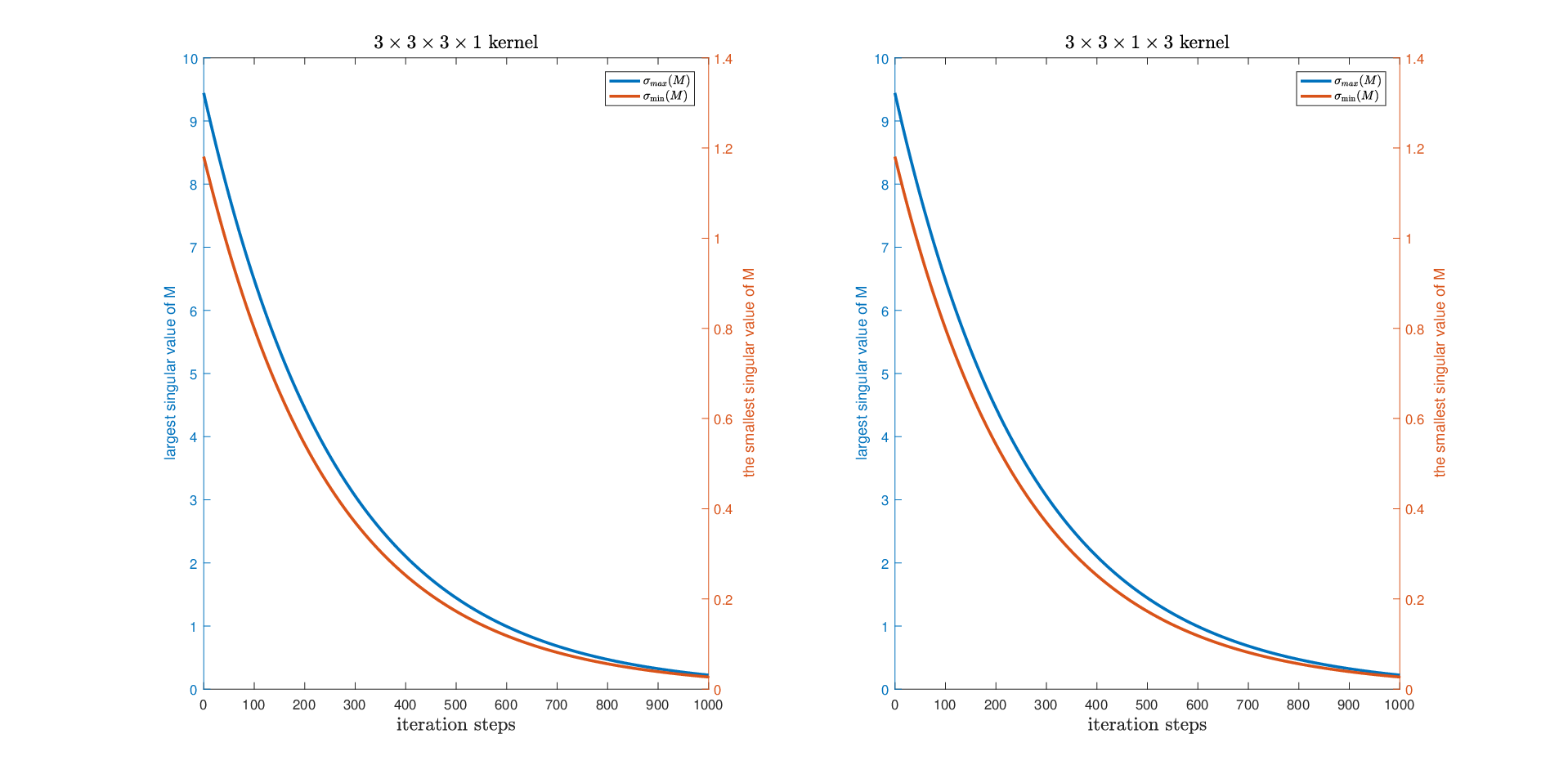
Numerical experiments are done on other random generated examples, including random kernels with each entry uniformly distributed on $[0,1]$. The convergence figures of $\sigma_{max}(M)$ and $\sigma_{min}(M)$ are similar with the subfigures presented in the paper.

The efficiency of each method, i.e., the needed iteration steps to let $\sigma_{max}(M)$ and $\sigma_{min}(M)$ be bounded in a satisfying interval, is related with the step size $\lambda$. In our numerical experiments, for Algorithms 3.1 and 3.3 we use the step size $\lambda=1e-5$ while for Algorithms 3.2 we use the step size $\lambda=1e-4$. We can’t definitely tell how to choose the optimal step size currently.

In this paper, we provide a new regularization method to regularize the weights of convolutional layers in deep neural networks. We give new regularization terms about convolutional kernels to change the singular values of the corresponding structured transformation matrices. We propose gradient decent algorithms for the regularization terms. This method is shown to be effective.

In future, we will continue to devise other forms of penalty functions for convolutional kernels to constrain the singular values of corresponding transformation matrices.

References

- [1] Andrew Brock, Theodore Lim, James M Ritchie, and Nick Weston. Neural photo editing with introspective adversarial networks. In ICLR, 2017.
- [2] R. Chan and X. Jin, An Introduction to Iterative Toeplitz Solvers, SIAM, Philadelphia, 2007.
- [3] Moustapha Cisse, Piotr Bojanowski, Edouard Grave, Yann Dauphin, Nicolas Usunier. Parseval Networks: Improving Robustness to Adversarial Examples. In ICML, 2017.
- [4] Vincent Dumoulin, Francesco Visin. A guide to convolution arithmetic for deep learning. ArXiv, 2018.
- [5] G.-H. Golub and C.-F. Van Loan, Matrix computations, Johns Hopkins University Press, Baltimore, 2012.
- [6] I. J. Goodfellow, J. Shlens, and C. Szegedy. Explaining and harnessing adversarial examples. In ICLR, 2015.
- [7] P. Guo, Q. Ye. On Regularization of Convolutional Kernels in Neural Networks, ArXiv 2019.
- [8] P. Guo. A Frobenius norm regularization method for convolutional kernels to avoid unstable gradient problem, ArXiv 2019.
- [9] S. Hochreiter, Y. Bengio, P. Frasconi, J. Schmidhuber, et al. Gradient flow in recurrent nets: the difficulty of learning long-term dependencies, In Field Guide to Dynamical Recurrent Networks, IEEE Press, 2001.
- [10] X. Jin, Developments and Applications of Block Toeplitz Iterative Solvers, Science Press, Beijing, 2002.
- [11] Kovaevi, Jelena and Chebira, Amina. An introduction to frames, Now Publishers Inc, Boston, 2008.
- [12] Takeru Miyato, Toshiki Kataoka, Masanori Koyama, Yuichi Yoshida. Spectral Normalization for Generative Adversarial Networks. In ICLR, 2018.
- [13] Hanie Sedghi, Vineet Gupta and Philip M. Long. The Singular Values of Convolutional Layers. In ICLR, 2019.
- [14] G. W. Stewart. Matrix Algorithms: Volume II. Eigensystems, SIAM, 2001.
- [15] C. Szegedy, W. Zaremba, I. Sutskever, J. Bruna, D. Erhan, I. J. Goodfellow, and R. Fergus. Intriguing properties of neural networks. In ICLR, 2014.
- [16] Y. Tsuzuku, I. Sato, and M. Sugiyama. Lipschitz-Margin Training: Scalable Certification of Perturbation Invariance for Deep Neural Networks. In NIPS, 2018.
- [17] Jiayun Wang, Yubei Chen, Rudrasis Chakraborty, and Stella X. Yu. Orthogonal Convolutional Neural Networks. ArXiv 2019
- [18] C. Zhang, S. Bengio, M. Hardt, B. Recht, and O. Vinyals. Understanding deep learning requires rethinking generalization. In ICLR, 2017.
- [19] Yuichi Yoshida, Takeru Miyato. Spectral Norm Regularization for Improving the Generalizability of Deep Learning, ArXiv 2017.