跳到论文正文
W Papers独立论文阅读器 arXiv:2102.04166 论文正文 计算阅读时间 · 0%
引用这篇论文根据当前论文元数据生成,正式投稿前建议核对。


License: CC BY 4.0
arXiv:2102.04166v2 [math.NA] 29 Jun 2021

Analysis and application of an overlapped FEM-BEM for wave propagation in unbounded and heterogeneous media

V. Domínguez Thanks: Department of Estadística, Informática y Matemáticas, Universidad Pública de Navarra, Tudela, Spain/ Institute for Advanced Materials (INAMAT), Pamplona, Spain. Email: victor.dominguez@unavarra.es    M. Ganesh Thanks: Department Applied Mathematics and Statistics Department, Colorado School of Mines, Golden, CO, USA. Email: mganesh@mines.edu
August 11, 2026
Abstract

An overlapped continuous model framework, for the Helmholtz wave propagation problem in unbounded regions comprising bounded heterogeneous media, was recently introduced and analyzed by the authors (J. Comput. Phys., 403, 109052, 2020). The continuous Helmholtz system incorporates a radiation condition (RC) and our equivalent hybrid framework facilitates application of widely used finite element methods (FEM) and boundary element methods (BEM), and the resulting discrete systems retain the RC exactly. The FEM and BEM discretizations, respectively, applied to the designed interior heterogeneous and exterior homogeneous media Helmholtz systems include the FEM and BEM solutions matching in artificial interface domains, and allow for computations of the exact ansatz based far-fields. In this article we present rigorous numerical analysis of a discrete two-dimensional FEM-BEM overlapped coupling implementation of the algorithm. We also demonstrate the efficiency of our discrete FEM-BEM framework and analysis using numerical experiments, including applications to non-convex heterogeneous multiple particle Janus configurations. Simulations of the far-field induced differential scattering cross sections (DSCS) of heterogeneous configurations and orientation-averaged (OA) counterparts are important for several applications, including inverse wave problems. Our robust FEM-BEM framework facilitates computations of such quantities of interest, without boundedness or homogeneity or shape restrictions on the wave propagation model.

Dedicated to the memory of Francisco-Javier “Pancho” Sayas (1968-2019).

AMS subject classifications: 65N30, 65N38, 65F10, 35J05

Keywords: Helmholtz, Heterogeneous, Unbounded, Wave Propagation, Finite Element Methods, Integral Equations, Nyström Boundary Element Methods, Janus Configurations

1 Introduction

Simulation of scattered acoustic and electromagnetic fields, and hence understanding the impact of refractive indices of wave propagation media, are crucial for a large class of applications [6, 24, 31, 33]. The term Janus particles was mentioned in a Nobel Prize lecture [9] about three decades ago, and since then additional interests include understanding the effect of a class of piecewise-continuous heterogeneous refractive indices induced Janus configurations. A simple Janus particle is designed by combining two distinct homogeneous refractive indices, and Janus configurations in general may comprise multiple particles or complex structures with heterogeneous material properties. The example configuration Ω0\Omega_{0}, of the type illustrated in Figure 1, has been investigated for synthesis and applications, see for example [29, 39, 38, 34].

Figure 1: An incident wave uincu^{\rm inc} impinging on a given Janus-type heterogeneous multiple-particle configuration (Ω0\Omega_{0}) in ℝ2\mathbb{R}^{2}. Our framework introduces two artificial boundaries Σ\Sigma and Γ\Gamma, and hence two overlapped computational regions: (i) a bounded FEM-domain Ω2\Omega_{2} (with boundary Σ\Sigma) and (ii) an unbounded BEM-region ℝ2∖Ω¯1\mathbb{R}^{2}\setminus\overline{\Omega}_{1} (exterior to the smooth interface Γ\Gamma). The FEM and BEM solutions are constrained to match in the overlapped region Ω12:=(ℝ2∖Ω¯1)∩Ω2{\Omega_{12}:=}(\mathbb{R}^{2}\setminus\overline{\Omega}_{1})\cap\Omega_{2}.

Developing numerical methods to understand scattering effects by Janus configurations (even with simple structures) has been an active area of research, see for example the Janus spherical acoustic configuration effect research [33, 21] published in 2020 and references therein. Motivated by details in the book [33], authors of [21] numerically investigated scattering effects of homogeneous spheres with two standard (sound-soft and transmission) boundary properties, leading to solving the Helmholtz equation with two distinct boundary conditions and the Sommerfeld radiation condition (SRC), for the unknown scattered- and far-fields.

As described in [33, 21], to understand the impact of Janus-type wave configurations, accurate simulations of certain quantities of interests (QoI) are important. The two key QoI are the far-field intensity based differential scattering cross sections (DSCS) and also the configuration orientation effect QoI, the orientation-averaged (OA) DSCS. Simulation of the OA-DSCS is equivalent to simulating far-fields generated by the configuration, such as Ω0\Omega_{0} in Figure 1, with the incident wave uincu^{\rm inc} impinging Ω0\Omega_{0} from hundreds of directions surrounding the configuration. The key numerical tool in [21] is the stable far-fields based T-matrix framework that was analyzed (with a priori bounds) and implemented in [14, 13]. For nonlinear inverse problems based applications that use the far-field (with phase or phase-less DSCS) data, efficient simulation of far-fields (such as at each Newton-type iterations) are important, see for example the 2019 book [6] and extensive references therein.

Far-field computations based numerical schemes for such QoI and tools, in general, do not allow for configurations with heterogeneous structures and unbounded regions. This is mainly because numerical partial differential equation (PDE) algorithms mainly apply either the ubiquitous finite element method (FEM) or the boundary element method (BEM). The FEM requires a bounded domain for finite number of tessellations, and the BEM requirement of the fundamental solution is practical mainly for a homogeneous medium PDE. The FEM is applied to a variational formulation equation of the PDE that involves domain integrals, and the BEM discretizes an equivalent boundary integral equation (BIE) for the boundary unknown in a chosen ansatz for the scattered field, in conjunction with the fundamental solution [6, 31].

Accordingly for wave propagation models with a bounded heterogeneous medium (Ω0\Omega_{0}), to apply the FEM, an artificial truncation of the unbounded region using, typically, a polygonal boundary Σ\Sigma (as in Figure 1) is introduced and a wave absorbing boundary condition (ABC) on Σ\Sigma is imposed, ignoring the SRC. The standard variational formulation on the boundary polygonal domain (such as Ω2\Omega_{2} in Figure 1) for the heterogeneous Helmholtz PDE with ABC on Σ\Sigma is sign-indefinite [24, 16] and this non-coercive restriction was removed recently by developing, analyzing, and implementing a new sign-definite variational formulation [17]. Another option to exactly incorporate the SRC is, for example, by ignoring the heterogeneity and consider instead the homogeneous model exterior to the polygonal boundary Σ\Sigma or exterior to a smooth boundary Γ\Gamma (as in Figure 1). The artificial smooth boundary choice is especially suitable for developing high-order spectrally accurate approximation of the scattered field in the homogeneous medium using high-order BEMs.

For Janus-type configurations, it is important to avoid restrictions in either of the above two options by using both the FEM and BEM. This can be achieved by appropriately coupling the FEM and BEM solutions, depending on the choices of the artificial boundaries to compute the interior (heterogeneous) and exterior (homogeneous) media solutions. Such FEM-BEM coupling mathematical frameworks have been developed and analyzed only by a few authors, but several researchers implemented the associated FEM-BEM computational frameworks.

The widely used FEM-BEM coupling is obtained by choosing one artificial (FEM appropriate) polygonal boundary Σ\Sigma, see for example the review article [36] and references therein. In addition to analysis difficulties [36], this approach introduces restricted regularity for the solution exterior to Σ\Sigma. The high-order regularity based (BEM appropriate) single smooth boundary choice Γ\Gamma was subsequently developed in [26, 27]. For recent implementations of the single artificial boundary based FEM-BEM framework with high-order accuracy we refer to [15, 16, 19], and associated analysis issues are highlighted in [15, Section 6]. Using two artificial interfaces a mathematical framework was developed over four decades ago in [25] and was subsequently used in [8, 22]. A domain-overlapped framework [illustrated in Figure 1 with overlapped region (ℝ2∖Ω¯1)∩Ω2(\mathbb{R}^{2}\setminus\overline{\Omega}_{1})\cap\Omega_{2}] was developed recently by the authors in [10] that takes advantage of a polygonal boundary (Σ\Sigma) required for a wide-class FEM, and a smooth boundary (Γ\Gamma) for high-order spectral BEM. Mathematical analysis of the continuous framework in [10] establishes the equivalence and regularity of the decomposed model.

In this work we present rigorous numerical analysis of the FEM-BEM adaptive coupling framework introduced in [10] for solving the Helmholtz acoustic/electromagnetic wave propagation problem on the plane with a bounded heterogeneous region, and demonstrate efficiency of the numerical algorithm for complex Janus-type heterogeneous configurations with computational experiments. The algorithm works on a suitable partition of the plane defined from a polygonal domain containing a smooth curve that surround all heterogeneity. The overlapped partition is made up of the bounded polygonal domain containing the heterogeneity, and the unbounded homogeneous region exterior to the smooth curve.

On the bounded domain of the partition we approximate the solution by a FEM with classical continuous piecewise polynomials on triangular grids, whereas a high-order Nyström BEM is used to compute the scattered wave in the unbounded region. Both solutions are coupled by demanding to coincide in the two artificial boundaries that ensures the FEM and BEM solutions matching in the intersecting common domain of the partition. We prove that the convergence of the scheme in natural norms is of the same order as the best approximations of the projection in the FEM and BEM finite dimensional spaces. In addition, since the Nyström method is super-algebraically convergent, only a relatively few degrees of freedom are required in the BEM solver to keep the error of the same order as the FEM solution, and hence the algorithm facilitates accurate far field, DSCS, and OA-DSCS computations.

The rest of this article is organized as follows: In Section 2, we recall the Helmholtz model and an equivalent decomposition decomposition framework, both at continuous level. In Section 3 we setup a discrete counterpart of the decomposition framework and the overlapped FEM-BEM algorithm. Rigorous numerical analysis of the FEM-BEM algorithm establishing optimal order convergence, of the hybridized numerical solutions, in Section 4 forms the main theoretical contribution of the article that include references to several results proven in the two Appendix sections of this article. In Section 5, we computationally demonstrate the described algorithm and theoretically analysis using three distinct sets of experiments, in conjunction with the theory and practical applicability, including implementation of the algorithm for multiple-particle Janus-type configurations with non-smooth solutions, and also for complex structured heterogeneous regions.

2 Helmholtz model and decomposition framework

Throughout the article, let nn be a piecewise-continuous refractive index with heterogeneity restricted to a bounded domain Ω0⊂ℝ2\Omega_{0}\subset\mathbb{R}^{2}, and in the exterior we take n|Ω0c≡1n|_{\Omega_{0}^{\rm c}}\equiv 1 so that the exterior Ω0c(:=ℝ2∖Ω0¯CLOSE\Omega_{0}^{\rm c}~(:=\mathbb{R}^{2}\setminus\overline{\Omega_{0}}) is a free-space unbounded medium.

The scattered field usu^{s} is induced by an incident wave uincu^{\rm inc} (with wavenumber k>0k>0) from the exterior region impinging on the heterogeneous medium Ω0\Omega_{0}. It is convenient to assume that that incident field satisfies the homogeneous Helmholtz equation Δ​v+k2​v=0\Delta v+k^{2}v=0 in all of the plane ℝ2\mathbb{R}^{2}, although it is sufficient to take it to satisfy outside of a compact set in ℝ2\mathbb{R}^{2} containing, say, a point-source. Physically appropriate incident waves such as the plane-wave and point-source have these properties.

We seek the total wave field u(:=us+uinc)∈Hloc1​(ℝ2)u~(:=u^{s}+u^{\rm inc})\in H^{1}_{\rm loc}(\mathbb{R}^{2}), representing acoustic or electromagnetic fields, satisfying the uniquely solvable problem governed by the variable coefficient Helmholtz equation and the SRC (with 𝒙^:=𝒙/|𝒙|∈𝕊1\widehat{\bm{x}}:=\bm{x}/|\bm{x}|\in\mathbb{S}^{1}):

|Δ​u+k2​n2​u=0,in ​ℝ2,∂𝒙^us−i​k​us=o(|𝒙|−1/2),as |𝒙|→∞.\left|\begin{array}[]{rcl}\Delta u+k^{2}n^{2}\>u&=&0,\quad\text{in }\mathbb{R}^{2},\\ \partial_{{\widehat{\bm{x}}}}u^{s}-\mathrm{i}k{u}^{s}&=&o(|{{\bm{x}}|^{-1/2}}),\quad\text{as }|{{\bm{x}}}|\to\infty.\end{array}\right. (2.1)

We note that in the heterogeneous medium Ω0\Omega_{0}, usu^{s} is the interior unknown field and is the solution of inhomogeneous Helmholtz equation with inhomogeneous term f=−(Δ​uinc+k2​n2​uinc)f=-(\Delta u^{\rm inc}+k^{2}n^{2}\>u^{\rm inc}). For the unknown scattered field usu^{s} exterior to Ω0\Omega_{0}, in (2.1), the SRC

lim|𝒙|→∞|𝒙|1/2​(∂us​(𝒙)∂𝒙^−i​k​us​(𝒙))=0.\lim_{|\bm{x}|\to\infty}|\bm{x}|^{1/2}\left(\frac{\partial u^{s}(\bm{x})}{\partial{\widehat{\bm{x}}}}-\mathrm{i}ku^{s}(\bm{x})\right)=0. (2.2)

holds uniformly in all directions 𝒙^=𝒙/|𝒙|∈𝕊1\widehat{\bm{x}}=\bm{x}/|\bm{x}|\in\mathbb{S}^{1}. The scattered field usu^{s} is a radiating field and, as a consequence of the SRC, its behavior at infinity is captured by the far-field u∞∈L2​(𝕊1)u^{\infty}\in L^{2}(\mathbb{S}^{1}), where

u∞​(𝒙^)=lim|𝒙|→∞|𝒙|1/2​e−i​k​|𝒙|​us​(𝒙).u^{\infty}(\widehat{\bm{x}})=\lim_{|\bm{x}|\to\infty}|\bm{x}|^{1/2}e^{-\mathrm{i}k|\bm{x}|}u^{s}(\bm{x}). (2.3)

For the total field uu induced by a plane wave with incident direction 𝒅^∈𝕊1\widehat{\bm{d}}\in\mathbb{S}^{1}, it is appropriate to denote the associated far-field as u∞​(𝒙^,𝒅^)=u∞​(θ,ϕ)u^{\infty}(\widehat{\bm{x}};\widehat{\bm{d}})=u^{\infty}(\theta;\phi), with 𝒙^=p⁡(θ)=(cos⁡θ,sin⁡θ)\widehat{\bm{x}}=p(\theta)={(\cos\theta,\sin\theta)} and 𝒅^=p⁡(ϕ)=(cos⁡ϕ,sin⁡ϕ)\widehat{\bm{d}}=p(\phi)={(\cos\phi,\sin\phi)}, for some θ,ϕ∈[0,2​π)\theta,\phi\in[0,2\pi). The single-incident plane wave QoI DSCS and multiple-incident plane waves QoI OA-DSCS are then given by [33, 21]

uDSCS​(θ,ϕ)=|u∞​(θ,ϕ)|2;uDSCSOA​(θ)=12​π​∫02​π|u∞​(θ,ϕ)|2​𝑑ϕ.u_{\rm DSCS}(\theta;\phi)=|u^{\infty}(\theta;\phi)|^{2};\qquad u^{\rm OA}_{\rm DSCS}(\theta)=\frac{1}{2\pi}\int_{0}^{2\pi}|u^{\infty}(\theta;\phi)|^{2}\,{\rm d}\phi. (2.4)

Clearly, computation of the uDSCSOAu^{\rm OA}_{\rm DSCS} with high-accuracy requires discretization of the above integral with over thousand discrete incident direction angles ϕ\phi, leading to solving the same number of Helmholtz model (2.1)-(2.2) for many distinct inputs. This motivates the difficulty of evaluating uDSCSOAu^{\rm OA}_{\rm DSCS} Janus-type configurations with piecewise-continuous refractive indices defined on non-trivial geometries.

For the given wave propagation problem (2.1), next we recall an equivalent decomposition framework introduced and analyzed in [10]. The framework introduce two artificial curves Γ\Gamma and Σ\Sigma with interior Ω1\Omega_{1} and Ω2\Omega_{2}, respectively, satisfying Ω¯0⊂Ω1⊂Ω¯1⊂Ω2\overline{\Omega}_{0}\subset\Omega_{1}\subset\overline{\Omega}_{1}\subset\Omega_{2}, with the assumption that Γ\Gamma is smooth and Σ\Sigma is a polygonal boundary. A sketch of the different domains is displayed in Figure 1. We denote henceforth Ω1c:=ℝ2∖Ω¯1\Omega_{1}^{\rm c}:=\mathbb{R}^{2}\setminus\overline{\Omega}_{1}. At continuous level, it is convenient to consider the decomposition framework using operators defined on classical Sobolev spaces. To this end, for a general domain D∈ℝ2D\in\mathbb{R}^{2} with boundary ∂D\partial D and for real mm, let Hm​(D)H^{m}(D) denote the classical Sobolev space.

We also consider Hs​(∂D)H^{s}(\partial D) which is well defined for any ss if DD is smooth. Recall that in this case the trace operator γ∂D:Hs+1/2​(D)→Hs​(∂D)\gamma_{\partial D}:H^{s+1/2}(D)\to H^{s}(\partial D) is continuous for any s>0s>0 as consequence of the Sobolev Trace Theorems, see for example [7] or [30, Ch 4].

For Lipschitz domains Ω\Omega with boundary Σ=∂Ω\Sigma=\partial\Omega, such as the chosen polygonal domain Ω2\Omega_{2}, Hs​(Σ)H^{s}(\Sigma) is defined only for s∈[−1,1]s\in[-1,1] [1, 20, 30]. We then commit a (slight) abuse of notation and set for s>1s>1

Hs​(Σ)={γΣ​u:u∈Hs+1/2​(D)}.H^{s}(\Sigma)=\left\{\gamma_{\Sigma}u\ :\ u\in H^{s+1/2}(D)\right\}. (2.5)

In (2.5) the open domain DD is chosen such that Σ⊂D¯\Sigma\subset\overline{D}, and the space is endowed with the image norm. It is known that the space is independent of DD and, for s∈(0,1)s\in(0,1), it is a classical Sobolev space. Thus, using the definitions, the trace operator γΣ:Hs+1/2​(D)→Hs​(Σ)\gamma_{\Sigma}:H^{s+1/2}(D)\to H^{s}(\Sigma) is continuous for s∈(0,1)∪(1,∞)s\in(0,1)\cup(1,\infty).

The decomposition framework starts with an interior and an exterior Helmholtz problem:

  • •

    (Interior Dirichlet Helmholtz problem in Ω2\Omega_{2} with polygonal boundary Σ\Sigma):
    Given fΣ∈H1/2​(Σ)f_{\Sigma}\in H^{1/2}(\Sigma), find ωint∈H1​(Ω2)\omega_{\rm int}\in H^{1}(\Omega_{2}) so that

    |Δ​ωint+k2​n2​ωint=0,in ​Ω2,γΣ​ωint=fΣ.\left|\begin{array}[]{rcl}\Delta\omega_{\rm int}+k^{2}n^{2}\>\omega_{\rm int}&=&0,\quad\text{in }\Omega_{2},\\ \gamma_{\Sigma}\omega_{\rm int}&=&f_{\Sigma}.\end{array}\right. (2.6)
  • •

    (Exterior Dirichlet Helmholtz problem in Ω1c\Omega_{1}^{\rm c} with smooth boundary Γ\Gamma):
    Given fΓ∈H1/2​(Γ)f_{\Gamma}\in H^{1/2}(\Gamma), find ωext∈Hloc1​(Ω1c)\omega_{\rm ext}\in H^{1}_{\rm loc}(\Omega_{1}^{\rm c}) so that

    |Δ​ωext+k2​ωext=0,in ​Ω1c,γΓ​ωext=fΓ,∂𝒙^ωext−i​k​ωext=o(|𝒙|−1/2).\left|\begin{array}[]{rcl}\Delta\omega_{\rm ext}+k^{2}\omega_{\rm ext}&=&0,\quad\text{in }\Omega_{1}^{\rm c},\\ \gamma_{\Gamma}\omega_{\rm ext}&=&f_{\Gamma},\\ \partial_{{\widehat{\bm{x}}}}\omega_{\rm ext}-{\rm i}k\omega_{\rm ext}&=&o({|\bm{x}|^{-1/2}}).\end{array}\right. (2.7)

The SRC in (2.7) ensures that the exterior Dirichlet problem is uniquely solvable [6, 31] for all wavenumbers kk. For the interior Dirichlet Helmholtz problem (2.6) the well-posedness does not hold for all wavenumbers kk [24], and throughout this article we assume that the wavenumber kk is such that ωint\omega_{\rm int} is the unique solution of (2.6). The well-posedness assumption for the interior Dirichlet Helmholtz problems in Ω2\Omega_{2} (and in the overlapped region Ω12:=Ω1c∩Ω2\Omega_{12}:=\Omega_{1}^{c}\cap\Omega_{2}) can be easily avoided, for example, by modifying the artificial boundaries Σ\Sigma and Γ\Gamma [10, Section 2.1].

It is convenient to use operators to describe the continuous decomposition framework. To this end, corresponding to the interior Dirichlet problem (2.6) we consider two operators KΩ2​Σ,KΓ​Σ\mathrm{K}_{\Omega_{2}\Sigma},\mathrm{K}_{\Gamma\Sigma}; and associated with the exterior problem (2.7) we consider two operators KΩ1c​Γ,KΣ​Γ\mathrm{K}_{\Omega_{1}^{\rm c}\Gamma},\mathrm{K}_{\Sigma\Gamma}. These pairs of operators are defined, using the unique solution ωint\omega_{\rm int} of (2.6) and ωext\omega_{\rm ext} of (2.7) and their traces respectively on Γ\Gamma and Σ\Sigma, as follows:

KΩ2​Σ​fΣ=ωint,KΓ​Σ​fΣ=γΓ​ωint;KΩ1c​Γ​fΓ=ωext,KΣ​Γ​fΓ=γΣ​ωext.\mathrm{K}_{\Omega_{2}\Sigma}f_{\Sigma}=\omega_{\rm int},\qquad\mathrm{K}_{\Gamma\Sigma}f_{\Sigma}=\gamma_{\Gamma}\omega_{\rm int};\qquad\quad\mathrm{K}_{\Omega_{1}^{\rm c}\Gamma}f_{\Gamma}=\omega_{\rm ext},\quad\mathrm{K}_{\Sigma\Gamma}f_{\Gamma}=\gamma_{\Sigma}\omega_{\rm ext}. (2.8)

In [10], the authors proved that the unique solution uu of (2.1) can be constructed in two steps as follows:

  1. 1.

    Find fΣ:Σ→ℂf_{\Sigma}:\Sigma\to\mathbb{C} and fΓ:Γ→ℂf_{\Gamma}:\Gamma\to\mathbb{C} so that

    |fΣ−KΣ​Γ​fΓ=γΣ​uinc,−KΓ​Σ​fΣ+fΓ=−γΓ​uinc.\left|\begin{array}[]{ccccrcl}f_{\Sigma}&-&\mathrm{K}_{\Sigma\Gamma}f_{\Gamma}&=&\gamma_{\Sigma}u^{\rm inc},\\ -\mathrm{K}_{\Gamma\Sigma}f_{\Sigma}&+&f_{\Gamma}&=&-\gamma_{\Gamma}u^{\rm inc}.\end{array}\right. (2.9a)
  2. 2.

    Construct

    u={KΩ2​ΣfΣ,in Ω2,KΩ1c​ΓfΓ+uinc,in Ω1c.u=\begin{cases}\mathrm{K}_{\Omega_{2}\Sigma}f_{\Sigma},\quad&\text{in $\Omega_{2}$},\\ \mathrm{K}_{\Omega_{1}^{\rm c}\Gamma}f_{\Gamma}+u^{\rm inc},\quad&\text{in $\Omega_{1}^{\rm c}$}.\end{cases} (2.9b)

The boundary unknowns system (2.9a) can be written in matrix-valued operator form as

(ℐ−𝒦)​[fΣfΓ]=[γΣ​uinc−γΓ​uinc],𝒦:=[KΣ​ΓKΓ​Σ].\left({\cal I}-{\cal K}\right)\begin{bmatrix}f_{\Sigma}\\ f_{\Gamma}\end{bmatrix}=\begin{bmatrix}[r]\gamma_{\Sigma}u^{\rm inc}\\ -\gamma_{\Gamma}u^{\rm inc}\end{bmatrix},\qquad{\cal K}:=\begin{bmatrix}&\mathrm{K}_{\Sigma\Gamma}\\ \mathrm{K}_{\Gamma\Sigma}&\end{bmatrix}. (2.10)

(ℐ{\cal I} is obviously the identity matrix operator.) It is not difficult to see that the off-diagonal block 𝒦:H0​(Σ)×H0​(Γ)→Hs​(Σ)×Hs​(Γ){\cal K}:H^{0}(\Sigma)\times H^{0}(\Gamma)\to H^{s}(\Sigma)\times H^{s}(\Gamma) is continuous for any s≥0s\geq 0[10].

The following result summarizes the equivalence of the decomposition framework to the original problem (2.1) at the continuous level.

Theorem 2.1.

Assume that the only solution to problem

|Δ​v+k2​v=0,in ​Ω12=Ω1∩Ω2c,γΓ​v=0,γΣ​v= 0\left|\begin{array}[]{rcl}\Delta v+k^{2}v&=&0,\quad\text{in }\Omega_{12}=\Omega_{1}\cap\Omega_{2}^{c},\\ \gamma_{\Gamma}v&=&0,\quad\gamma_{\Sigma}v\,=\,0\end{array}\right. (2.11)

is the trivial one. Then ℐ−𝒦:Hs​(Σ)×Hs​(Γ)→Hs​(Σ)×Hs​(Γ){\cal I}-{\cal K}:H^{s}(\Sigma)\times H^{s}(\Gamma)\to H^{s}(\Sigma)\times H^{s}(\Gamma) is invertible for any s≥0s\geq 0. Therefore (2.9a) is uniquely solvable. Furthermore, uu defined by (2.9b) is the unique solution of the full Helmholtz problem (2.1).

Proof.

This result is proven in [10]. We will give here a sketch of the proof for the sake of completeness. By Fredholm alternative it suffices to show that ℐ−𝒦{\cal I}-{\cal K} is one-to-one. We note that any if (fΣ∗,fΓ∗)∈N⁡(ℐ−𝒦)(f_{\Sigma}^{*},f_{\Gamma}^{*})\in N({\cal I}-{\cal K}) then ω12:=(KΩ2​Σ​fΣ∗−KΩ1c​Γ​fΓ∗)|Ω12\omega_{12}:=(\mathrm{K}_{\Omega_{2}\Sigma}f_{\Sigma}^{*}-\mathrm{K}_{\Omega_{1}^{\rm c}\Gamma}f_{\Gamma}^{*})|_{\Omega_{12}} is a solution for (2.11). By hypothesis, ω12=0\omega_{12}=0. Hence, uu in (2.9b) is well defined for uinc=0u^{\rm inc}=0. The well-posedness of the scattering problem (2.1), implies that u=0u=0. In particular, KΩ1c​Γ​fΓ∗|Ω2c=0\mathrm{K}_{\Omega_{1}^{\rm c}\Gamma}f_{\Gamma}^{*}{|_{\Omega_{2}^{c}}}=0, and from the analytic continuation principle KΩ1c​Γ​fΓ⋆=0\mathrm{K}_{\Omega_{1}^{\rm c}\Gamma}{f^{\star}_{\Gamma}}=0. Therefore, also KΩ2​Σ​fΣ∗|Ω12=0{\mathrm{K}_{\Omega_{2}\Sigma}f_{\Sigma}^{*}|_{\Omega_{12}}}=0 and hence (fΣ∗,fΓ∗)=𝟎(f_{\Sigma}^{*},f_{\Gamma}^{*})={\bf 0}. ∎

Remark 2.2.

For the OA-DSCS calculations with a large number of incident plane waves uincu^{\rm inc}, a marked advantage of our equivalent formulation (2.9a)-(2.9b) compared to the original model problem (2.1) [with a large number of inhomogeneous terms f=−(Δ​uinc+k2​n2​uinc)f=-(\Delta u^{\rm inc}+k^{2}n^{2}\>u^{\rm inc}) in Ω0\Omega_{0}] is that the interior and exterior homogeneous problems KΩ2​Σ​fΣ,KΩ1c​Γ​fΓ\mathrm{K}_{\Omega_{2}\Sigma}f_{\Sigma},\mathrm{K}_{\Omega_{1}^{\rm c}\Gamma}f_{\Gamma} (and hence their traces KΓ​Σ​fΣ,KΣ​Γ​fΓ\mathrm{K}_{\Gamma\Sigma}f_{\Sigma},\mathrm{K}_{\Sigma\Gamma}f_{\Gamma}) can be setup independently of the incident waves. Since the unknowns fΣf_{\Sigma} and fΓf_{\Gamma} are defined, respectively, only on boundary curves Σ\Sigma and Γ\Gamma, these unknowns can represented by a few boundary unknowns (or boundary basis functions) and hence the associated Helmholtz problems setup KΩ2​Σ​fΣ,KΩ1c​Γ​fΓ\mathrm{K}_{\Omega_{2}\Sigma}f_{\Sigma},\mathrm{K}_{\Omega_{1}^{\rm c}\Gamma}f_{\Gamma} is a naturally parallel process for computational purposes.

3 Discrete decomposition FEM-BEM framework

The numerical discretization of the continuous decomposition framework (2.9) is essentially obtained by replacing the four continuous operators in (2.8) using appropriate FEM and BEM based discrete counterparts. For KΩ2​Σ\mathrm{K}_{\Omega_{2}\Sigma} we will use the standard FEM with continuous piecewise polynomial elements on a triangular conformal mesh of Ω2\Omega_{2} [24].

For the BEM certainly an extensive range of methods is at our disposal in the literature [6, 31]. We will restrict ourselves to the spectrally accurate Nyström method [28, 6] .This scheme provides a discretization of the key boundary integral operators of the associated Calderon calculus; in this article we will use only make use of the discrete Single- and Double-Layer operators that converge super-algebraically, and it is not difficult to implement. A disadvantage of the Nyström method is that it requires an accurate differentiable parameterization of the boundary. This is because the method is based on splitting the integral operators into regular and singular parts for which appropriate decompositions and factorizations of the kernels of the operators are needed. This is not a severe restriction in our case since Γ\Gamma is an auxiliary user-chosen artificial curve and therefore can be taken to be simple and smooth.

In the next two subsections we recall the standard FEM and Nyström procedure and conclude this section with the discrete FEM-BEM decomposition framework required for the main focus of this work on the numerical analysis of the FEM-BEM algorithm [10] .

The FEM procedure

Let {𝒯h}h\{\mathcal{T}_{h}\}_{h} be a sequence of regular triangular meshes with hh denoting the discrete parameter, the diameter of the largest element of the grid. We then write h→0h\to 0 to mean that the maximum of the diameters of the elements tends to 0. A technical mesh assumption, not restrictive in practice, described in detail in Assumption 1 below, will be used in our proofs to ensure (i) a faster convergence of the FEM in stronger norms around Γ\Gamma (see Theorem B.1 in Appendix); and (ii) the stability of the full method.

On 𝒯h{\cal T}_{h}, we construct the finite dimensional FEM space

ℙh,d:={vh∈𝒞0(Ω2):uh|Th∈ℙd,∀Th∈𝒯h},\mathbb{P}_{h,d}:=\{{v}_{h}\in{\cal C}^{0}(\Omega_{2}):\ u_{h}|_{T_{h}}\in\mathbb{P}_{d},\ \forall T_{h}\in{\cal T}_{h}\},

where ℙd\mathbb{P}_{d} is the space of bivariate polynomial of degree dd. Then given fΣh∈γΣ​ℙh,df_{\Sigma}^{h}\in\gamma_{\Sigma}\mathbb{P}_{h,d}, we define

KΩ2​Σh:γΣ​ℙh,d→ℙh,d\mathrm{K}_{\Omega_{2}\Sigma}^{h}:\gamma_{\Sigma}\mathbb{P}_{h,d}\to\mathbb{P}_{h,d}

as KΩ2​Σh​fΣh:=uh\mathrm{K}_{\Omega_{2}\Sigma}^{h}f_{\Sigma}^{h}:=u_{h} that is the unique of the standard FEM discrete system:

|uh∈ℙh,dbk,n​(uh,vh)=0,∀vh∈ℙh,d∩H01​(Ω2)γΣ​uh=fΣh,bk,n(u,v):=∫Ω2∇u⋅∇v−k2∫Ω2n2uv.\left|\begin{array}[]{l}u_{h}\in\mathbb{P}_{h,d}\\ b_{k,n}(u_{h},v_{h})=0,\quad\forall v_{h}\in\mathbb{P}_{h,d}\cap H_{0}^{1}(\Omega_{2})\\ \gamma_{\Sigma}u_{h}=f_{\Sigma}^{h},\end{array}\right.\qquad b_{k,n}(u,v):=\int_{\Omega_{2}}\nabla u\cdot\nabla v-k^{2}\int_{\Omega_{2}}n^{2}\,uv. (3.1)

It is well known that KΩ2​Σh\mathrm{K}_{\Omega_{2}\Sigma}^{h} [24] is well defined for any sufficiently fine mesh. Notice also that KΩ2​Σh\mathrm{K}_{\Omega_{2}\Sigma}^{h} is defined on the discrete space γΣ​ℙh,d\gamma_{\Sigma}\mathbb{P}_{h,d}, the trace finite element space on the boundary Σ\Sigma. Hence, with the help of

QΣh:𝒞0​(Σ)→γΣ​ℙh,d,{\rm Q}^{h}_{\Sigma}:{\cal C}^{0}(\Sigma)\to\gamma_{\Sigma}\mathbb{P}_{h,d}, (3.2)

the nodal interpolation operator on γΣ​ℙh,d\gamma_{\Sigma}\mathbb{P}_{h,d} defined by the finite element space, we have

KΩ2​Σh​QΣh≈KΩ2​Σ,\mathrm{K}_{\Omega_{2}\Sigma}^{h}{\rm Q}^{h}_{\Sigma}\approx\mathrm{K}_{\Omega_{2}\Sigma},

providing an optimal approximation in ℙh,d\mathbb{P}_{h,d} for sufficiently smooth Dirichlet data fΣhf_{\Sigma}^{h} (see Theorem 4.1 in the next section).

The BEM procedure

Let

𝐱=(x1​(t),x2​(t)):ℝ→Γ{\bf x}=(x_{1}(t),x_{2}(t)):\mathbb{R}\to\Gamma (3.3)

be a smooth 2​π−2\pi-periodic parameterization of Γ\Gamma. We denote by SLk{\rm SL}_{k}, DLk{\rm DL}_{k}, the (parameterized) layer potentials, defined for 𝒛∈ℝ2∖Γ{\bm{z}}\in\mathbb{R}^{2}\setminus\Gamma as,

(SLk​φper)​(𝒛)\displaystyle({\rm SL}_{k}\varphi_{{\rm per}})({\bm{z}}) :⁣=\displaystyle:= ∫02​πΦk​(𝒛−𝐱⁡(t))​φper​(t)​𝑑t,\displaystyle\int_{0}^{2\pi}\Phi_{k}({\bm{z}}-{\bf x}(t))\varphi_{{\rm per}}(t)\,{\rm d}t,\,\quad
(DLk​gper)​(𝒛)\displaystyle({\rm DL}_{k}g_{{\rm per}})({\bm{z}}) :⁣=\displaystyle:= ∫02​π(∇𝒚Φk​(𝒛−𝒚))|𝒚=𝐱⁡(t)⋅𝝂⁡(t)​gper​(t)​𝑑t,\displaystyle\int_{0}^{2\pi}\big(\nabla_{\bm{y}}\Phi_{k}({\bm{z}}-{\bm{y}})\big)\Big|_{{\bm{y}}={\bf x}(t)}\cdot\bm{\nu}(t)\,g_{{\rm per}}(t)\,{\rm d}t,

where Φk=i4H0(1)(k|⋅|)\Phi_{k}=\frac{\rm i}{4}H_{0}^{(1)}(k|\cdot|) is the fundamental solution for the constant coefficient Helmholtz operator in ℝ2\mathbb{R}^{2} with wavenumber kk; 𝝂⁡(t):=(x2′​(t),−x1′​(t))\bm{\nu}(t):=(x_{2}^{\prime}(t),-x_{1}^{\prime}(t)) is a non-normalized normal vector. Observe that |𝐱′​(t)|>0|{\bf x}^{\prime}(t)|>0 is then incorporated to the density in SLk{\rm SL}_{k} and to the kernel in DLk{\rm DL}_{k}. We follow the same convention for the single and double boundary operator defined for 2​π2\pi-periodic densities φper\varphi_{{\rm per}} and gperg_{{\rm per}} as

(Vk​φper)​(s)\displaystyle\hskip-21.68121pt(\mathrm{V}_{k}\varphi_{{\rm per}})(s)\hskip-7.22743pt :⁣=\displaystyle:= (γΓ​SLk​φper)​(𝐱⁡(s))=∫02​πΦk​(𝐱⁡(s)−𝐱⁡(t))​φper​(t)​𝑑t\displaystyle\left(\gamma_{\Gamma}{\rm SL}_{k}\varphi_{{\rm per}}\right)({\bf x}(s))=\int_{0}^{2\pi}\Phi_{k}({\bf x}(s)-{\bf x}(t))\varphi_{{\rm per}}(t)\,{\rm d}t\,\quad (3.4)
(Kk​gper)​(s)\displaystyle\hskip-21.68121pt(\mathrm{K}_{k}g_{{\rm per}})(s)\hskip-7.22743pt :⁣=\displaystyle:= ±12​gper​(s)+(γΓ∓​DLk​gper)​(s)=∫02​π(∇𝒚Φk​(𝐱⁡(s)−𝒚))|𝒚=𝐱⁡(t)⋅𝝂⁡(t)​gper​(t)​𝑑t.\displaystyle\pm\tfrac{1}{2}g_{{\rm per}}(s)+(\gamma^{\mp}_{\Gamma}{\rm DL}_{k}g_{{\rm per}})(s)=\int_{0}^{2\pi}\big(\nabla_{{\bm{y}}}\Phi_{k}({\bf x}(s)-{\bm{y}})\big)\Big|_{{\bm{y}}={\bf x}(t)}\hskip-10.84006pt\cdot\bm{\nu}(t)\,g_{{\rm per}}(t)\,{\rm d}t. (3.5)

The Brakhage-Werner formulation, first introduced in [3] (see also [6, 31]) provides a robust representation for the solution of the exterior Dirichlet solution for the Helmholtz problem (2.7):

KΩ1c​Γ​fΓ=(DLk−i​k​SLk)​(12​I+Kk−i​k​Vk)−1​(fΓ∘𝐱),\mathrm{K}_{\Omega_{1}^{\rm c}\Gamma}f_{\Gamma}=({\rm DL}_{k}-{\rm i}k{\rm SL}_{k})(\tfrac{1}{2}\mathrm{I}+\mathrm{K}_{k}-\mathrm{i}k\mathrm{V}_{k})^{-1}(f_{\Gamma}\circ{\bf x}), (3.6)

with I\mathrm{I} obviously being the identity operator. The above representation of the exterior scattered field, satisfying the SRC, provides an exact ansatz for the associated far-field as (ℱ​φper)​(𝒛^),𝒛^∈𝕊1({\cal{F\varphi}}_{\rm per})({\widehat{\bm{z}}}),~\widehat{\bm{z}}\in\mathbb{S}^{1} defined, using the boundary density φper=(12​I+Kk−i​k​Vk)−1​(fΓ∘𝐱)\varphi_{\rm per}=(\tfrac{1}{2}\mathrm{I}+\mathrm{K}_{k}-\mathrm{i}k\mathrm{V}_{k})^{-1}(f_{\Gamma}\circ{\bf x}) [6]:

(ℱ​φper)​(𝒛^):=k8​π​exp⁡(−14​π​i)​∫02​πexp⁡(−i​k​(𝒛^⋅𝐱⁡(t)))​[𝒛^⋅(x2′​(t),−x1′​(t))+1]​φper​(t)​𝑑t.\left({\cal F}\varphi_{\rm per}\right)(\widehat{\bm{z}}):=\sqrt{\frac{k}{8\pi}}\exp\big(-\tfrac{1}{4}\pi{\rm i}\big)\int_{0}^{2\pi}\exp(-\mathrm{i}k(\widehat{\bm{z}}\cdot{\bf x}(t)))\big[\widehat{\bm{z}}\cdot(x_{2}^{\prime}(t),-x_{1}^{\prime}(t))+1\big]\varphi_{\rm per}(t)\,{\rm d}t. (3.7)

Thus accurate computational approximations of φper\varphi_{\rm per} provide spectrally accurate approximations for both the scattered and the far-field. For computing φper\varphi_{\rm per}, the Nyström BEM solver makes use of a decomposition of the single- and double- layer operator into logarithmic and regular parts:

(Vk​φper)​(s)\displaystyle({\rm V}_{k}\varphi_{{\rm per}})(s) =\displaystyle= ∫02​πA⁡(s,t)​log⁡sin2⁡s−t2​φper​(t)​𝑑t+∫02​πB⁡(s,t)​φper​(t)​𝑑t,\displaystyle\int_{0}^{2\pi}A(s,t)\log\sin^{2}\tfrac{s-t}{2}\>\varphi_{{\rm per}}(t)\>{\rm d}t+\int_{0}^{2\pi}B(s,t)\varphi_{{\rm per}}(t)\>{\rm d}t,
(Kk​gper)​(s)\displaystyle({\rm K}_{k}g_{{\rm per}})(s) =\displaystyle= ∫02​πC⁡(s,t)​log⁡sin2⁡s−t2​gper​(t)​𝑑t+∫02​πD⁡(s,t)​gper​(t)​𝑑t.\displaystyle\int_{0}^{2\pi}C(s,t)\log\sin^{2}\tfrac{s-t}{2}\>g_{{\rm per}}(t)\>{\rm d}t+\int_{0}^{2\pi}D(s,t)g_{{\rm per}}(t)\>{\rm d}t.

Functions A,B,C,DA,\ B,\ C,\ D are smooth and 2​π−2\pi-biperiodic.

Next with NN being a positive integer BEM discretization parameter, we consider the grid

{tj}j∈ℤ⊂ℝ,tj:=j​πN,\{t_{j}\}_{j\in\mathbb{Z}}\subset\mathbb{R},\quad t_{j}:=\tfrac{j\pi}{N},

and the 2​N2N-dimensional space of trigonometric polynomials defined by

𝕋N:=span⟨eℓ:ℓ∈ℤN⟩,eℓ(t):=exp(iℓt)\mathbb{T}_{N}:=\spann\langle e_{\ell}\ :\ \ell\in\mathbb{Z}_{N}\rangle,\quad e_{\ell}(t):=\exp({\rm i}\ell t) (3.8)

where ℤN={−N+1,−N+2,…,N}\mathbb{Z}_{N}=\{-N+1,-N+2,\ldots,N\}. The interpolation operator for 2​π−2\pi-periodic functions φper\varphi_{{\rm per}}

𝕋N∋QN​φpers.t.(QN​φper)​(tj)=φper​(tj),\mathbb{T}_{N}\ni\mathrm{Q}_{N}\varphi_{{\rm per}}\quad\text{s.t.}\quad(\mathrm{Q}_{N}\varphi_{{\rm per}})(t_{j})=\varphi_{{\rm per}}(t_{j}),

is known to be well defined.

The Nyström method is based on the following approximations for the single- and double-layer operators:

(VkN​φper)​(s)\displaystyle({\rm V}_{k}^{N}\varphi_{{\rm per}})(s) :⁣=\displaystyle:= ∫02​πQN​(A⁡(s,⋅)​φper)​(t)​log⁡sin2⁡s−t2​𝑑t+∫02​πQN​(B⁡(s,⋅)​φper)​(t)​𝑑t\displaystyle\int_{0}^{2\pi}{\rm Q}_{N}(A(s,\cdot)\varphi_{{\rm per}}\big)(t)\log\sin^{2}\tfrac{s-t}{2}\>{\rm d}t+\int_{0}^{2\pi}{\rm Q}_{N}(B(s,\cdot)\varphi_{{\rm per}}\big)(t)\>{\rm d}t
(KkN​gper)​(s)\displaystyle({\rm K}_{k}^{N}g_{\rm per})(s) :⁣=\displaystyle:= ∫02​πQN​(C⁡(s,⋅)​gper)​(t)​log⁡sin2⁡s−t2​𝑑t+∫02​πQN​(D⁡(s,⋅)​gper)​(t)​𝑑t.\displaystyle\int_{0}^{2\pi}{\rm Q}_{N}(C(s,\cdot)g_{\rm per}\big)(t)\log\sin^{2}\tfrac{s-t}{2}\>{\rm d}t+\int_{0}^{2\pi}{\rm Q}_{N}(D(s,\cdot)g_{\rm per}\big)(t)\>{\rm d}t.

We stress that the integrals above can be computed exactly. Indeed,

−12​π∫02​πlogsin2t2en(t)dt=−12​π∫02​πlogsin2t2cos(nt)dt={log⁡4,n=01|n|,n≠0,-\frac{1}{2\pi}\int_{0}^{2\pi}\log\sin^{2}\tfrac{t}{2}\>e_{n}(t)\>{\rm d}t=-\frac{1}{2\pi}\int_{0}^{2\pi}\log\sin^{2}\tfrac{t}{2}\cos(nt)\>{\rm d}t=\begin{cases}\log 4,&n=0\\ \frac{1}{|n|},&n\neq 0,\end{cases}

and

∫02​π(QN​gper)​(t)​𝑑t=πN​∑j=02​N−1(QN​gper)​(tj)=πN​∑j=02​N−1gper​(tj),\int_{0}^{2\pi}(\mathrm{Q}_{N}g_{\rm per})(t)\>{\rm d}t=\frac{\pi}{N}\sum_{j=0}^{2N-1}(\mathrm{Q}_{N}g_{\rm per})(t_{j})=\frac{\pi}{N}\sum_{j=0}^{2N-1}g_{\rm per}(t_{j}),\qquad

i.e., for the regular part the suggested approximation yields the trapezoidal/rectangular rule for 2​π−2\pi-periodic functions.

The evaluation of the potentials, as integral operators with smooth kernel, is carried out in a similar way:

(SLkN​φper)​(𝒛)\displaystyle\big({\rm SL}_{k}^{N}\varphi_{{\rm per}}\big)({\bm{z}}) :=∫02​πQN​(Φk​(𝒛−𝐱⁡(⋅))​φper)​(t)​𝑑t\displaystyle:=\ \int_{0}^{2\pi}{\rm Q}_{N}(\Phi_{k}({\bm{z}}-{\bf x}(\cdot))\varphi_{{\rm per}})(t)\,{\rm d}t (3.9)
(DLkN​gper)​(𝒛)\displaystyle\big({\rm DL}_{k}^{N}g_{\rm per}\big)({\bm{z}}) :=∫02​πQN​((∇𝒚Φk​(𝒛−𝒚))|𝒚=𝐱⁡(⋅)⋅𝝂⁡(⋅)​gper)​(t)​dt.\displaystyle:=\ \int_{0}^{2\pi}{\rm Q}_{N}\big(\big(\nabla_{\bm{y}}\Phi_{k}({\bm{z}}-{\bm{y}})\big)\big|_{{\bm{y}}={\bf x}(\cdot)}\cdot\bm{\nu}(\cdot)\,g_{\rm per})(t)\,{\rm d}t.

We are ready to present the discrete version for KΩ1c​Γh\mathrm{K}_{\Omega_{1}^{\rm c}\Gamma}^{h}. Hence, in view of

KΩ1c​Γ​fΓ=(DLk−i​k​SLk)​ℒk​(fΓ∘𝐱),with ​ℒk:=(12​I+Kk−i​k​Vk)−1,\mathrm{K}_{\Omega_{1}^{\rm c}\Gamma}f_{\Gamma}=({\rm DL}_{k}-{\rm i}k{\rm SL}_{k}){\cal L}_{k}(f_{\Gamma}\circ{\bf x}),\quad\text{with }{\cal L}_{k}:=(\tfrac{1}{2}\mathrm{I}+\mathrm{K}_{k}-\mathrm{i}k\mathrm{V}_{k})^{-1}, (3.10)

we define for fper:=fΓ∘𝐱f_{\rm per}:=f_{\Gamma}\circ{\bf x}

KΩ1c​ΓN​fper:=(DLkN−i​k​SLkN)​ℒkN​fper,with ​ℒkN:=(12​I+KkN−i​k​VkN)−1.\mathrm{K}_{\Omega_{1}^{\rm c}\Gamma}^{N}{f_{\rm per}}:=(\mathrm{DL}_{k}^{N}-{\rm i}k\mathrm{SL}_{k}^{N}){\cal L}_{k}^{N}{f_{\rm per}},\quad\text{with }{\cal L}_{k}^{N}:=(\tfrac{1}{2}\mathrm{I}+\mathrm{K}_{k}^{N}-\mathrm{i}k\mathrm{V}_{k}^{N})^{-1}. (3.11)

Hence φperN:=ℒkN​fper\varphi_{\rm per}^{N}:={\cal L}_{k}^{N}f_{\rm per} is the spectrally accurate approximation to the density φ=ℒk​fΓ\varphi={\cal L}_{k}f_{\Gamma}. In addition, we can also introduce the associated far-field approximation, see (3.7), as

(ℱN​φperN)​(𝒛^):=k8​π​exp⁡(−14​π​i)​πN​∑j=−N+1Nexp⁡(−i​k​(𝒛^⋅𝐱⁡(tj)))​[𝒛^⋅(x2′​(tj),−x1′​(tj))+1]​φperN​(tj).\left({\mathcal{F}}_{N}{\varphi}_{{\rm per}}^{N}\right)(\widehat{\bm{z}}):=\sqrt{\frac{k}{8\pi}}\exp\big(-\tfrac{1}{4}\pi{\rm i}\big)\frac{\pi}{N}\sum_{j=-N+1}^{N}\exp(-\mathrm{i}k(\widehat{\bm{z}}\cdot{\bf x}(t_{j})))\big[\widehat{\bm{z}}\cdot(x_{2}^{\prime}(t_{j}),-x_{1}^{\prime}(t_{j}))+1\big]{\varphi}_{{\rm per}}^{N}(t_{j}). (3.12)
Remark 3.1.

It is not difficult to show that

φperN=ℒkN​fper⇒QN​φperN=QN​ℒkN​QN​fper.\varphi^{N}_{\rm per}={\cal L}_{k}^{N}f_{\rm per}\quad\Rightarrow\quad{\rm Q}_{N}\varphi^{N}_{\rm per}={\rm Q}_{N}{\cal L}_{k}^{N}{\rm Q}_{N}f_{\rm per}.

We note that only pointwise values of the density φper\varphi_{\rm per} are used for computation of the BEM-based potentials and QoI. Accordingly, we can conclude that the true unknowns of the Nyström method are the values of the density at the grid points {φper​(tj)}j∈ℤ\{\varphi_{\rm per}(t_{j})\}_{j\in\mathbb{Z}} and that such values are computed by the algorithm using only the values of the right-hand-side fperf_{\rm per} at the same grid.

The BEM-FEM coupling method

Let

KΣ​ΓN:=γΣ​KΩ1c​ΓN,KΓ​Σh:=(γΓ​KΩ2​Σh)∘𝐱,\mathrm{K}_{\Sigma\Gamma}^{N}:=\gamma_{\Sigma}\mathrm{K}_{\Omega_{1}^{\rm c}\Gamma}^{N},\quad\mathrm{K}_{\Gamma\Sigma}^{h}:=(\gamma_{\Gamma}\mathrm{K}_{\Omega_{2}\Sigma}^{h})\circ{\bf x},

be the discrete counterparts of KΣ​Γ\mathrm{K}_{\Sigma\Gamma} and KΓ​Σ\mathrm{K}_{\Gamma\Sigma}. That is, the first operator computes the BEM solution and evaluate on the outer polygonal domain Σ\Sigma, whereas the second one solves the FEM problem and evaluates it on the interior and smooth Γ\Gamma.

Then our coupled FEM-BEM algorithm is:

  • •

    Solve

    (fΣh,fperN)∈\displaystyle(f^{h}_{\Sigma},f^{N}_{\rm per})\in γΣ​ℙh,d×𝕋Ns.t.\displaystyle\gamma_{\Sigma}\mathbb{P}_{h,d}\times\mathbb{T}_{N}\quad\text{s.t.} (3.13a)
    (ℐ−[QΣh​KΣ​ΓNQN​KΓ​Σh])​[fΣhfperN]=[QΣh​γΣ​uinc−QN​γΓ​(uinc∘𝐱)].\displaystyle\left({\cal I}-\begin{bmatrix}&{\rm Q}^{h}_{\Sigma}\mathrm{K}_{\Sigma\Gamma}^{N}\\ {\rm Q}_{N}\mathrm{K}_{\Gamma\Sigma}^{h}\end{bmatrix}\right)\begin{bmatrix}f^{h}_{\Sigma}\\ f^{N}_{\rm per}\end{bmatrix}=\begin{bmatrix}[r]{\rm Q}^{h}_{\Sigma}\gamma_{\Sigma}u^{\rm inc}\\ -{\rm Q}_{N}\gamma_{\Gamma}(u^{\rm inc}\circ{\bf x})\end{bmatrix}.
  • •

    Construct

    wh=KΩ2​Σh​fΣh,ωN=KΩ1c​ΓN​fperN,uh,N={wh,in Ω2,ωN+uinc,in Ω1c.w_{h}=\mathrm{K}_{\Omega_{2}\Sigma}^{h}f_{\Sigma}^{h},\quad\omega_{N}=\mathrm{K}_{\Omega_{1}^{\rm c}\Gamma}^{N}f^{N}_{\rm per},\quad u_{h,N}=\begin{cases}w_{h},\quad&\text{in $\Omega_{2}$},\\ \omega_{N}+u^{\rm inc},\quad&\text{in $\Omega_{1}^{\rm c}$}.\end{cases} (3.13b)
Remark 3.2.

In view of Remark 3.1, for implementation of the above algorithm, the pointwise values of the numerical solution (fΣh,fperN)(f^{h}_{\Sigma},f^{N}_{\rm per}) at the boundary nodes (of the FEM and BEM grids on Σ\Sigma and Γ\Gamma) are the true unknowns. Hence  (3.13a) leads to a relatively small algebraic system.

We also note that, in view of the first-stage coupled and constrained solutions in (3.13a), the overlapped algorithm is designed in such a way that for sufficiently fine grids, the final-stage FEM and BEM parts of the algorithm in (3.13b) lead to two numerically coinciding solutions in Ω12=Ω1c∩Ω2\Omega_{12}=\Omega_{1}^{\rm c}\cap\Omega_{2}. (We demonstrate this property using numerical experiments.)

4 Numerical analysis of overlapped FEM-BEM algorithm

We analyze the above FEM-BEM scheme through rigorous derivation of the stability and convergence estimates in appropriate Sobolev norms. For the polygonal region we keep using the standard space Hs​(Ω1)H^{s}(\Omega_{1}) and Hs​(Σ)H^{s}(\Sigma) (with the convention (2.5) for s>1s>1). For the smooth boundary Γ\Gamma, since we switch to the parameterized spaced (via 𝐱{\bf x}), we will work with 2​π−2\pi-periodic Sobolev spaces. To this end, we define

Hpers:={φper∈𝒟′(ℝ):φper=φper(⋅+2π),∥φper∥Hpers<∞}.H^{s}_{{\rm per}}:=\{\varphi_{{\rm per}}\in{\cal D}^{\prime}(\mathbb{R})\ :\ \varphi_{{\rm per}}=\varphi_{{\rm per}}(\,\cdot\,+2\pi),\ \|\varphi_{{\rm per}}\|_{H^{s}_{{\rm per}}}<\infty\}. (4.1)

In (4.1), the distribution elements in the space are continuous linear functionals on 𝒟⁡(ℝ){\cal D}(\mathbb{R}) (where 𝒟⁡(ℝ){\cal D}(\mathbb{R}) is the space of the smooth compactly supported functions in ℝ\mathbb{R} endowed with its natural topology), and the space is equipped with the norm

‖φper‖Hpers2=|φper​(0)|2+∑n≠0|n|2​s​|φ^per​(n)|2,\|\varphi_{{\rm per}}\|_{H^{s}_{{\rm per}}}^{2}=|\varphi_{{\rm per}}(0)|^{2}+\sum_{n\neq 0}|n|^{2s}|\widehat{\varphi}_{{\rm per}}(n)|^{2}, (4.2)

where φ^per​(n)\widehat{\varphi}_{{\rm per}}(n) is the nnth Fourier coefficient:

φ^per​(n):=∫02​πφper​(t)​e−n​(t)​𝑑t.\widehat{\varphi}_{{\rm per}}(n):=\int_{0}^{2\pi}{\varphi}_{{\rm per}}(t)e_{-n}(t)\,{\rm d}t.

It is a well established result that Hs​(Γ)H^{s}(\Gamma) and HpersH^{s}_{\rm per} are isomorphic via the composition with 𝐱{\bf x} (see for example [28, Th. 8.13]).

4.1 Interpolation and some projection operators on the discrete spaces

For the implementation as well as for the theoretical analysis, we need some projections onto the discrete spaces defined on the boundaries Σ\Sigma and Γ\Gamma. In the first case we have already introduced the Lagrange interpolation operator in ℙh,d\mathbb{P}_{h,d} (see (3.2)). For such operators it can be shown, as consequence of well-known results, that

‖QΣh​fΣ−fΣ‖Hs​(Σ)≤C​hΣt−s​‖fΣ‖Ht​(Σ)\|{\rm Q}^{h}_{\Sigma}f_{\Sigma}-f_{\Sigma}\|_{H^{s}(\Sigma)}\leq Ch_{\Sigma}^{t-s}\|f_{\Sigma}\|_{H^{t}(\Sigma)} (4.3a)
where CC depends only on Σ\Sigma, s∈[0,1]s\in[0,1] and s≤t<d+1s\leq t<d+1 and t>1/2t>1/2. Here and in what follows hΣh_{\Sigma} is the maximum of the diameters of elements in Σ\Sigma induced by the mesh 𝒯h{\cal T}_{h}. The convergence of order hΣd+1−sh_{\Sigma}^{d+1-s} can be attained if we assume an extra regularity for fΣf_{\Sigma}: for any s∈[0,1]s\in[0,1] and t>d+1t>d+1, there exists CC so that
‖QΣh​fΣ−fΣ‖Hs​(Σ)≤C​hΣd+1−s​‖fΣ‖Ht​(Σ).\|{\rm Q}^{h}_{\Sigma}f_{\Sigma}-f_{\Sigma}\|_{H^{s}(\Sigma)}\leq Ch_{\Sigma}^{d+1-s}\|f_{\Sigma}\|_{H^{t}(\Sigma)}. (4.3b)

We refer the reader to Appendix A for proofs of such results. In this section we also introduce a more flexible projection on γΣ​ℙhd\gamma_{\Sigma}\mathbb{P}_{h}^{d}, which will be required for analysis purposes. Roughly speaking this is a consequence of carrying out the analysis in H1​(Ω)H^{1}(\Omega) and H1/2​(Σ)H^{1/2}(\Sigma) norms which, although are the natural ones for the FEM method, contains discontinuous functions and for which the action of QΣh{\rm Q}^{h}_{\Sigma} cannot be therefore considered. Hence, we claim that there exists PΣh:H1/2​(Σ)→γΣ​ℙh,d{\rm P}_{\Sigma}^{h}:H^{1/2}(\Sigma)\to\gamma_{\Sigma}\mathbb{P}_{h,d} a projection on γΣ​ℙh,d\gamma_{\Sigma}\mathbb{P}_{h,d} satisfying

‖PΣh​fΣ−fΣ‖Hs​(Σ)\displaystyle\|{\rm P}_{\Sigma}^{h}f_{\Sigma}-f_{\Sigma}\|_{H^{s}(\Sigma)} ≤\displaystyle\leq C​hΣt−s​‖fΣ‖Ht​(Σ),0≤s<1,s≤t<d+1,t≥1/2.\displaystyle Ch_{\Sigma}^{t-s}\|f_{\Sigma}\|_{H^{t}(\Sigma)},\quad 0\leq s<1,\quad s\leq t<d+1,\quad t\geq 1/2. (4.4a)
‖PΣh​fΣ−fΣ‖Hs​(Σ)\displaystyle\|{\rm P}_{\Sigma}^{h}f_{\Sigma}-f_{\Sigma}\|_{H^{s}(\Sigma)} ≤\displaystyle\leq C​hΣd+1−s​‖fΣ‖Ht​(Σ),0≤s<1,t>d+1.\displaystyle Ch_{\Sigma}^{d+1-s}\|f_{\Sigma}\|_{H^{t}(\Sigma)},\quad 0\leq s<1,\quad t>d+1. (4.4b)

Proofs of the estimates (4.3) and (4.4) are given in Proposition A.1 and A.3 respectively in Appendix A.

The convergence of the trigonometric interpolation operator in the Sobolev frame is a well known result, see for example, [35, Th. 8.3.1]:

‖QN​φper−φper‖Hpers≤C​Ns−t​‖φper‖Hpert,\|\mathrm{Q}_{N}\varphi_{{\rm per}}-\varphi_{{\rm per}}\|_{H_{\rm per}^{s}}\leq CN^{s-t}\|\varphi_{{\rm per}}\|_{H_{\rm per}^{t}}, (4.5)

for any t≥s≥0t\geq s\geq 0 and t>1/2t>1/2, where CC depends only on s,ts,t. For similar reasons, and again only for our analysis, we use the L2L^{2}-projection, which turns out to be the HsH^{s}-orthogonal projection for any ss, on 𝕋N\mathbb{T}_{N}:

𝕋N∋PN​φper,s.t.PN​φper^​(n)=φper^​(n),n∈ℤN.\mathbb{T}_{N}\ni\mathrm{P}_{N}\varphi_{{\rm per}},\quad\text{s.t.}\quad\widehat{{\rm P}_{N}\varphi_{{\rm per}}}(n)=\widehat{\varphi_{{\rm per}}}(n),\quad n\in\mathbb{Z}_{N}.

It is straightforward to show that for any t≥st\geq s,

‖PN​φper−φper‖Hpers≤Ns−t​‖φper‖Hpert.\|\mathrm{P}_{N}\varphi_{{\rm per}}-\varphi_{{\rm per}}\|_{H_{\rm per}^{s}}\leq N^{s-t}\|\varphi_{{\rm per}}\|_{H_{\rm per}^{t}}. (4.6)

With the help of these two projections we define

𝒦h,N:=[QΣh​KΣ​ΓN​PNQN​KΓ​Σh​PΣh]{\cal K}_{h,N}:=\begin{bmatrix}&{\rm Q}_{\Sigma}^{h}\mathrm{K}_{\Sigma\Gamma}^{N}{\rm P}_{N}\\ {\rm Q}_{N}\mathrm{K}_{\Gamma\Sigma}^{h}{\rm P}_{\Sigma}^{h}&\end{bmatrix} (4.7)

so that the (3.13a) can be set up as

(ℐ−𝒦h,N)​[fΣfper]=[gΣgper]({\cal I}-{\cal K}_{h,N})\begin{bmatrix}f_{\Sigma}\\ f_{{\rm per}}\end{bmatrix}=\begin{bmatrix}g_{\Sigma}\\ g_{{\rm per}}\end{bmatrix}

for appropriate (gΣ,gper)⊤∈H1/2​(Σ)×Hper1/2(g_{\Sigma},g_{{\rm per}})^{\top}\in H^{1/2}(\Sigma)\times H_{{\rm per}}^{1/2}. Observe that in the case that the right-hand-side (gΣ,gper)(g_{\Sigma},g_{{\rm per}}) belongs to the discrete space γΣ​ℙh,d×𝕋N\gamma_{\Sigma}\mathbb{P}_{h,d}\times\mathbb{T}_{N} (as in (3.13a)), so is the solution (fΣ,fper)(f_{\Sigma},f_{{\rm per}}). In this case, PΣh{\rm P}_{\Sigma}^{h} and PN{\rm P}_{N} in (4.7) are already acting on elements on the discrete space and can safely removed. Thus the role of these projections is to facilitate the analysis by setting up the equation in the continuous framework.

4.2 Convergence for the FEM scheme

We recall some classical convergence results as well as superconvergence phenomenon for the FEM solution in the following theorem.

Theorem 4.1.

For fixed gΣ∈H1/2​(Σ)g_{\Sigma}\in\ H^{1/2}(\Sigma), gΣh∈γΣ​ℙh,dg_{\Sigma}^{h}\in\gamma_{\Sigma}\mathbb{P}_{h,d}, let

u:=KΩ2​Σ​gΣ,uh:=KΩ2​Σh​gΣh,u:=\mathrm{K}_{\Omega_{2}\Sigma}g_{\Sigma},\quad u_{h}:=\mathrm{K}_{\Omega_{2}\Sigma}^{h}g_{\Sigma}^{h},

be the solution of the interior Helmholtz problem (2.6) and the approximation given by the FEM (3.1). Then there exists C>0C>0 independent of gΣg_{\Sigma}, gΣhg_{\Sigma}^{h} and hh so that

‖u−uh‖H1​(Ω2)≤C⁡[infvh∈ℙh,d‖u−vh‖H1​(Ω2)+‖gΣ−gΣh‖H1/2​(Σ)].\|u-u_{h}\|_{H^{1}({\color[rgb]{0,0,0}\Omega_{2}})}\leq C\Big[\inf_{v_{h}\in\mathbb{P}_{h,d}}\|u-v_{h}\|_{H^{1}({\color[rgb]{0,0,0}\Omega_{2}})}+\|g_{\Sigma}-g_{\Sigma}^{h}\|_{H^{1/2}(\Sigma)}\Big]. (4.8)

Furthermore, let D′D^{\prime}, DD be domains with D′⊂D¯′⊂D⊂D¯⊂Ω2∖Ω0¯D^{\prime}\subset\overline{D}^{\prime}\subset D\subset\overline{D}\subset\Omega_{2}\setminus\overline{\Omega_{0}} and {𝒯h}h\{{\cal T}_{h}\}_{h} be a sequence of regular grids with h→0h\to 0 which are quasi-uniform in DD, that is

minK∈𝒯KK∩D≠∅⁡hK≥c​maxM∈𝒯hM∩D≠∅​hM,\min_{\begin{subarray}{c}K\in\mathcal{T}_{K}\\ K\cap D\neq\emptyset\end{subarray}}h_{K}\geq c\max_{\begin{subarray}{c}M\in\mathcal{T}_{h}\\ M\cap D\neq\emptyset\end{subarray}}h_{M}, (4.9)

for some constant cc independent of levels of discretization. Then there exists δ∈(1/2,1]\delta\in(1/2,1] such that for any ε∈[0,1/2)\varepsilon\in[0,1/2) and for any fine enough grid 𝒯h{\cal T}_{h},

‖u−uh‖H1+ε​(D′)≤C⁡[(hδ​hD−ε+hD1−ε)​‖u−uh‖H1​(Ω2)+hD−ε​‖gΣ−gΣh‖L2​(Σ)+hDd−ε​‖u‖Hd+1​(D)]\|u-u_{h}\|_{H^{1+\varepsilon}(D^{\prime})}\leq C\big[(h^{\delta}h^{-\varepsilon}_{D}+h_{D}^{1-\varepsilon})\|u-u_{h}\|_{H^{1}({\color[rgb]{0,0,0}\Omega_{2}})}+h^{-\varepsilon}_{D}\|g_{\Sigma}-g_{\Sigma}^{h}\|_{L^{2}(\Sigma)}+h_{D}^{d-\varepsilon}\|u\|_{H^{d+1}(D)}\big] (4.10)

with C>0C>0 depending on ε\varepsilon, DD and D′D^{\prime}, and hDh_{D} being the maximum of the diameters of the elements of the grid contained in DD.

Proof.

For (4.8) we refer to [37] (see also [11]). Estimate (4.10) can be derived using the superconvergence of the FEM solution in the interior of the computational domain where the solution is smooth (actually analytic) cf. [32]. We give a proof of these results in Corollary B.3 in Appendix B for the sake of completeness. ∎

Let us point out that the constant δ∈(1/2,1]\delta\in(1/2,1] in (4.10) depends on the regularity of the dual problem with homogeneous Dirichlet condition and a right-hand-side in L2​(Ω)L^{2}(\Omega). Therefore, for convex polygonal domains in ℝ2\mathbb{R}^{2}, we can take δ=1\delta=1 [20].

Assumption 1

Assume that for some open domain D⊂Ω2∖Ω¯0D\subset\Omega_{2}\setminus\overline{\Omega}_{0} with Γ⊂D\Gamma\subset D there exists ε0>0\varepsilon_{0}>0 such that the sequence of grids {𝒯h}h\{{\cal T}_{h}\}_{h} is quasi-uniform in DD and satisfies

h1/2​hD−ε0→0h^{1/2}h_{D}^{-\varepsilon_{0}}\to 0

where hDh_{D} is the maximum of the diameters of the elements of the grid 𝒯h{\cal T}_{h} having non-empty intersection with DD. □\Box

We note that this assumption allows locally refined grids but introduces a very weak restriction on the ratio between the larger element in Ω2\Omega_{2} and the smaller element in DD. However, since the exact solution is smooth on DD, it is reasonable to expect that small elements are not going to be used in this subdomain.

Lemma 4.2.

Let DD and the sequence of grids {𝒯h}\{{\cal T}_{h}\} be as in Assumption 1. Then, for any open subset D′D^{\prime} of DD containing Γ\Gamma and for any ε∈[0,1/2)\varepsilon\in[0,1/2), there exists C>0C>0 such that

‖KΓ​Σ​fΣ−KΓ​Σh​PΣh​fΣ‖Hper1/2+ε\displaystyle\|\mathrm{K}_{\Gamma\Sigma}f_{\Sigma}-\mathrm{K}_{\Gamma\Sigma}^{h}{\rm P}^{h}_{\Sigma}f_{\Sigma}\|_{H^{1/2+\varepsilon}_{{\rm per}}}
≤\displaystyle\leq C​h1/2​hD−ε​[infvh∈ℙh,d‖KΩ2​Σ​fΣ−vh‖H1​(Ω2)+‖fΣ−PΣh​fΣ‖H1/2​(Σ)]+C​hDd−ε​‖fΣ‖L2​(Σ).\displaystyle Ch^{1/2}h_{D}^{-\varepsilon}\big[\inf_{v_{h}\in\mathbb{P}_{h,d}}\|\mathrm{K}_{\Omega_{2}\Sigma}f_{\Sigma}-v_{h}\|_{{\color[rgb]{0,0,0}H^{1}(\Omega_{2})}}+\|f_{\Sigma}-{\rm P}^{h}_{\Sigma}f_{\Sigma}\|_{H^{1/2}(\Sigma)}\big]+Ch_{D}^{d-\varepsilon}\|f_{\Sigma}\|_{L^{2}(\Sigma)}.
Proof.

Notice that

‖fΣ−PΣh​fΣ‖L2​(Σ)=‖fΣ−PΣh​fΣ−PΣh​(fΣ−PΣh​fΣ)‖L2​(Σ)≤C​h1/2​‖fΣ−PΣh​fΣ‖H1/2​(Σ).\|f_{\Sigma}-{\rm P}^{h}_{\Sigma}f_{\Sigma}\|_{L^{2}(\Sigma)}=\|f_{\Sigma}-{\rm P}^{h}_{\Sigma}f_{\Sigma}-{\rm P}^{h}_{\Sigma}(f_{\Sigma}-{\rm P}^{h}_{\Sigma}{f_{\Sigma}})\|_{L^{2}(\Sigma)}\leq Ch^{1/2}\|f_{\Sigma}-{\rm P}^{h}_{\Sigma}f_{\Sigma}\|_{H^{1/2}(\Sigma)}.

Take D′D^{\prime} so that Γ⊂D′⊂D¯′⊂D\Gamma\subset D^{\prime}\subset\overline{D}^{\prime}\subset D. We claim that there exist CC independent of fΣf_{\Sigma}, so that

‖KD​Σ​fΣ‖Hd+1​(D)≤C​‖fΣ‖L2​(Σ).\|\mathrm{K}_{D\Sigma}f_{\Sigma}\|_{H^{d+1}(D)}\leq C\|f_{\Sigma}\|_{L^{2}(\Sigma)}. (4.11)

This can be seen as consequence of that the differential equations in DD becomes the homogeneous Helmholtz equation and Γ\Gamma is sufficiently far away from the boundary of DD.

The continuity of the trace operator γΓ:H1+ε​(D′)→H1/2+ε​(Γ)∼Hper1/2+ε\gamma_{\Gamma}:H^{1+\varepsilon}(D^{\prime})\to H^{1/2+\varepsilon}(\Gamma)\sim H^{1/2+\varepsilon}_{{\rm per}} and a direct application of (4.8-4.10) yield

∥KΓ​ΣfΣ−\displaystyle\|\mathrm{K}_{\Gamma\Sigma}f_{\Sigma}- KΓ​ΣhPhΣfΣ∥Hper1/2+ε\displaystyle\mathrm{K}_{\Gamma\Sigma}^{h}{\rm P}^{h}_{\Sigma}f_{\Sigma}\|_{H^{1/2+\varepsilon}_{{\rm per}}}
≤\displaystyle\leq C⁡(hδ​hD−ε+hD1−ε+h1/2−ε)​[infvh∈ℙh,d‖KΩ2​Σ​fΣ−vh‖H1​(Ω2)+‖fΣ−PΣh​fΣ‖H1/2​(Σ)]\displaystyle C(h^{\delta}h_{D}^{-\varepsilon}+h_{D}^{1-\varepsilon}+h^{1/2-\varepsilon})\big[\inf_{v_{h}\in\mathbb{P}_{h,d}}\|\mathrm{K}_{\Omega_{2}\Sigma}f_{\Sigma}-v_{h}\|_{H^{1}(\Omega_{2})}+\|f_{\Sigma}-{\rm P}^{h}_{\Sigma}f_{\Sigma}\|_{H^{1/2}(\Sigma)}\big]
+C​hDd−ε​‖fΣ‖L2​(Σ).\displaystyle+Ch_{D}^{d-\varepsilon}\|f_{\Sigma}\|_{L^{2}(\Sigma)}.

Using that δ≥1/2\delta\geq 1/2 the result is proven. ∎

We are ready to prove the convergence, in operator norm, of the first off diagonal block in (4.7) to the corresponding one in (2.10)

Proposition 4.3.

For any 0<ε≤ε00<\varepsilon\leq\varepsilon_{0} and for any t≥0t\geq 0 there exists C>0C>0 independent of fΣf_{\Sigma}, hh and NN such that

∥KΓ​ΣfΣ\displaystyle\|\mathrm{K}_{\Gamma\Sigma}f_{\Sigma} −QNKΓ​ΣhPhΣfΣ∥Hper1/2\displaystyle-{\rm Q}_{N}\mathrm{K}_{\Gamma\Sigma}^{h}{\rm P}^{h}_{\Sigma}f_{\Sigma}\|_{H^{1/2}_{{\rm per}}} (4.12)
≤\displaystyle\leq C⁡(1+N−ε​hD−ε)​h1/2​[infvh∈ℙh,d‖KΩ2​Σ​fΣ−vh‖H1​(Ω2)+‖fΣ−PΣh​fΣ‖H1/2​(Σ)]\displaystyle C\big(1+N^{-\varepsilon}h_{D}^{-\varepsilon}\big)h^{1/2}\big[\inf_{v_{h}\in\mathbb{P}_{h,d}}\|\mathrm{K}_{\Omega_{2}\Sigma}f_{\Sigma}-v_{h}\|_{H^{1}(\Omega_{2})}+\|f_{\Sigma}-{\rm P}^{h}_{\Sigma}f_{\Sigma}\|_{H^{1/2}(\Sigma)}\big]
+C⁡(N−ε​hDd−ε+hDd+N−t)​‖fΣ‖L2​(Σ).\displaystyle+C(N^{-\varepsilon}h_{D}^{d-\varepsilon}+h_{D}^{d}+N^{-t})\|f_{\Sigma}\|_{L^{2}(\Sigma)}.

In particular, we have the convergence in operator norm:

‖KΓ​Σ−QN​KΓ​Σh​PΣh‖H1/2​(Σ)→Hper1/2→0as ​(N,h)→(∞,0).\|\mathrm{K}_{\Gamma\Sigma}-{\rm Q}_{N}\mathrm{K}_{\Gamma\Sigma}^{h}{\rm P}^{h}_{\Sigma}\|_{H^{1/2}(\Sigma)\to H^{1/2}_{{\rm per}}}\to 0\quad\text{as }(N,h)\to(\infty,0). (4.13)
Proof.

The identity

KΓ​Σ−QN​KΓ​Σh​PΣh=(I−QN)​KΓ​Σ+(I−QN)​(KΓ​Σh​PΣh−KΓ​Σ)+(KΓ​Σ−KΓ​Σh​PΣh),\mathrm{K}_{\Gamma\Sigma}-{\rm Q}_{N}\mathrm{K}_{\Gamma\Sigma}^{h}{\rm P}^{h}_{\Sigma}=\big({\rm I}-{\rm Q}_{N}\big)\mathrm{K}_{\Gamma\Sigma}+({\rm I}-{\rm Q}_{N})\big(\mathrm{K}_{\Gamma\Sigma}^{h}{\rm P}^{h}_{\Sigma}-\mathrm{K}_{\Gamma\Sigma}\big)+\big(\mathrm{K}_{\Gamma\Sigma}-\mathrm{K}_{\Gamma\Sigma}^{h}{\rm P}^{h}_{\Sigma}\big), (4.14)

and the estimates

‖(I−QN)​KΓ​Σ​fΣ‖Hper1/2\displaystyle\|({\rm I}-{\rm Q}_{N})\mathrm{K}_{\Gamma\Sigma}f_{\Sigma}\|_{H^{1/2}_{{\rm per}}} ≤\displaystyle\leq C​N−t​‖KΓ​Σ​fΣ‖Hpert+1/2≤C′​N−t​‖fΣ‖L2​(Σ)\displaystyle CN^{-t}\|\mathrm{K}_{\Gamma\Sigma}f_{\Sigma}\|_{H^{t+1/2}_{{\rm per}}}\leq C^{\prime}N^{-t}\|f_{\Sigma}\|_{{\color[rgb]{0.68,0,0}L^{2}(\Sigma)}}
‖(I−QN)​(KΓ​Σh​PΣh−KΓ​Σ)​fΣ‖Hper1/2\displaystyle\|({\rm I}-{\rm Q}_{N})(\mathrm{K}_{\Gamma\Sigma}^{h}{\rm P}^{h}_{\Sigma}-\mathrm{K}_{\Gamma\Sigma}\big)f_{\Sigma}\|_{H^{1/2}_{{\rm per}}} ≤\displaystyle\leq Cε1​N−ε1​‖(KΓ​Σh​PΣh−KΓ​Σ)​fΣ‖Hper1/2+ε1,\displaystyle C_{\varepsilon_{1}}N^{-{\varepsilon_{1}}}\|(\mathrm{K}_{\Gamma\Sigma}^{h}{\rm P}^{h}_{\Sigma}-\mathrm{K}_{\Gamma\Sigma}\big)f_{\Sigma}\|_{H^{1/2+{\varepsilon_{1}}}_{{\rm per}}},

which are consequences of (4.5) and (4.11), yield

‖KΓ​Σ​fΣ−QN​KΓ​Σh​PΣh​fΣ‖Hper1/2≤Cε​N−ε1​‖(KΓ​Σh​PΣh−KΓ​Σ)​fΣ‖Hper1/2+ε1+C′​N−t​‖fΣ‖L2​(Σ)+‖(KΓ​Σh​PΣh−KΓ​Σ)​fΣ‖Hper1/2\|\mathrm{K}_{\Gamma\Sigma}f_{\Sigma}-{\rm Q}_{N}\mathrm{K}_{\Gamma\Sigma}^{h}{\rm P}^{h}_{\Sigma}f_{\Sigma}\|_{H^{1/2}_{{\rm per}}}\\ \leq C_{\varepsilon}N^{-\varepsilon_{1}}\|(\mathrm{K}_{\Gamma\Sigma}^{h}{\rm P}^{h}_{\Sigma}-\mathrm{K}_{\Gamma\Sigma}\big)f_{\Sigma}\|_{H^{1/2+\varepsilon_{1}}_{{\rm per}}}+C^{\prime}N^{-t}\|f_{\Sigma}\|_{{\color[rgb]{0.68,0,0}L^{2}(\Sigma)}}+\|(\mathrm{K}_{\Gamma\Sigma}^{h}{\rm P}^{h}_{\Sigma}-\mathrm{K}_{\Gamma\Sigma}\big)f_{\Sigma}\|_{H^{1/2}_{{\rm per}}}

Applying Lemma 4.2 twice (with ε=ε1\varepsilon=\varepsilon_{1} for the first term and ε=0\varepsilon=0 for the third one) yield (4.12). Consequently, (4.13) follows. ∎

4.3 Convergence for the BEM scheme

The inverse inequality

‖φperN‖Hpert≤Nt−s​‖φperN‖Hpers,t≥s,∀φperN∈𝕋N,\|\varphi_{{\rm per}}^{N}\|_{H^{t}_{{\rm per}}}\leq N^{t-s}\|\varphi_{{\rm per}}^{N}\|_{H^{s}_{{\rm per}}},\quad t\geq s,\quad\forall\varphi_{{\rm per}}^{N}\in\mathbb{T}_{N}, (4.15)

that is straightforward to derive from (3.8) and (4.2), will be used repeatedly in this section. The first result in this subsection summarizes the convergence of the BEM solver in a format that will be used later. This is based on the convergence in norm of the approximation operator ℒkN{\cal L}_{k}^{N} to the continuous counterpart. We recall that ℒk:Hpers→Hpers{\cal L}_{k}:H^{s}_{{\rm per}}\to H^{s}_{{\rm per}} is continuous for any s∈ℝs\in\mathbb{R}.

Theorem 4.4.

Fix t≥s>1/2t\geq s>1/2. Then, there exists C>0C>0 such that for any NN large enough and for any fper∈Hpertf_{\rm per}\in H^{t}_{\rm per},

‖ℒk​fper−ℒkN​fper‖Hpers≤C​Ns−t−α​‖fper‖Hpert,with ​α=min⁡{s,1}.\|{\cal L}_{k}f_{\rm per}-{\cal L}_{k}^{N}f_{\rm per}\|_{H_{\rm per}^{s}}\leq CN^{s-t-\alpha}\|f_{\rm per}\|_{H_{\rm per}^{t}},\qquad\text{with }\alpha=\min\{s,1\}. (4.16)

Therefore, ℒkN:Hpers→Hpers{\cal L}_{k}^{N}:H^{s}_{{\rm per}}\to H^{s}_{{\rm per}} is uniformly continous in NN for any s>1/2s>1/2.

Moreover, for s,t≥0s,t\geq 0, with t≥max⁡{s−1,0}t\geq\max\{s-1,0\} there exits C>0C>0 such that, for NN large enough,

‖QN​ℒk​PN​fper−QN​ℒkN​PN​fper‖Hpers≤C​Ns−t−α​‖PN​fper‖Hpert≤C​Ns−t−α​‖fper‖Hpert.\|\mathrm{Q}_{N}{\cal L}_{k}\mathrm{P}_{N}f_{\rm per}-\mathrm{Q}_{N}{\cal L}_{k}^{N}\mathrm{P}_{N}f_{\rm per}\|_{H_{\rm per}^{s}}\leq CN^{s-t-\alpha}\|{\mathrm{P}_{N}f_{\rm per}}\|_{H_{\rm per}^{t}}\leq CN^{s-t-\alpha}\|f_{\rm per}\|_{H_{\rm per}^{t}}. (4.17)
Proof.

The estimates, recall (3.10) and (3.11),

‖KkN−Kk‖Hpert→Hpers+‖VkN−Vk‖Hpert→Hpers≤C​Ns−t−α\|\mathrm{K}_{k}^{N}-\mathrm{K}_{k}\|_{H_{\rm per}^{t}\to H_{\rm per}^{s}}+\|\mathrm{V}_{k}^{N}-\mathrm{V}_{k}\|_{H_{\rm per}^{t}\to H_{\rm per}^{s}}\leq CN^{s-t-\alpha}

with s,t,αs,\ t,\ \alpha as in the statement of the Theorem (see Chapter 12 and 13 in [28] or, for a more detailed proof, [12, Th. 3.1]) proves that ℒkN:Hpers→Hpers{\cal L}_{k}^{N}:H_{\rm per}^{s}\to H_{\rm per}^{s} for s>1/2s>1/2 is well defined, for NN large enough, and it is uniformly bounded. Estimate (4.16) follows now from the identity

ℒk−ℒkN=ℒkN​[(ℒkN)−1−ℒk−1]​ℒk=ℒkN​[(KkN−Kk)−i​k​(VkN−Vk)]​ℒk.{\cal L}_{k}-{\cal L}_{k}^{N}={\cal L}_{k}^{N}\big[\big({\cal L}_{k}^{N})^{-1}-{\cal L}_{k}^{-1}\big]{\cal L}_{k}={\cal L}_{k}^{N}\big[(\mathrm{K}^{N}_{k}-\mathrm{K}_{k})-{\rm i}k(\mathrm{V}_{k}^{N}-\mathrm{V}_{k})\big]{\cal L}_{k}.

To prove the second estimate (4.17), we proceed in two steps: For s∈[1,∞)s\in[1,\infty), t≥s−1t\geq s-1 we have

‖QN​ℒkN​PN​fper−QN​ℒk​PN​fper‖Hpers\displaystyle\|\mathrm{Q}_{N}{\cal L}_{k}^{N}\mathrm{P}_{N}f_{\rm per}-\mathrm{Q}_{N}{\cal L}_{k}\mathrm{P}_{N}f_{\rm per}\|_{H_{\rm per}^{s}} ≤\displaystyle\leq C​‖(ℒkN−ℒk)​PN​fper‖Hpers≤C′​Ns−t−2​‖PN​fper‖Hpert+1\displaystyle C\|({\cal L}_{k}^{N}-{\cal L}_{k})\mathrm{P}_{N}f_{\rm per}\|_{H_{\rm per}^{s}}\leq C^{\prime}N^{s-t-2}\|\mathrm{P}_{N}f_{\rm per}\|_{H_{\rm per}^{t+1}} (4.18)
≤\displaystyle\leq C′​Ns−t−1​‖PN​fper‖Hpert.\displaystyle C^{\prime}N^{s-t-1}\|\mathrm{P}_{N}f_{\rm per}\|_{H_{\rm per}^{{t}}}.

(Notice that in the last step we have used the inverse inequality (4.15).) On the other hand, for s∈[0,1]s\in[0,1] and t≥0t\geq 0, we make use of the bound ‖QN​gper‖Hper0≤C​‖gper‖Hper1\|{\rm Q}_{N}g_{{\rm per}}\|_{H_{\rm per}^{0}}\leq C\|g_{{\rm per}}\|_{H_{\rm per}^{1}} to derive

‖QN​ℒkN​PN​fper−QN​ℒk​PN​fper‖Hpers\displaystyle\|\mathrm{Q}_{N}{\cal L}_{k}^{N}\mathrm{P}_{N}f_{{\rm per}}-\mathrm{Q}_{N}{\cal L}_{k}\mathrm{P}_{N}f_{{\rm per}}\|_{H_{\rm per}^{s}} ≤\displaystyle\leq C​‖(ℒkN−ℒk)​PN​fper‖Hper1≤C′​N−t−1​‖PN​fper‖Hpert+1\displaystyle C\|({\cal L}_{k}^{N}-{\cal L}_{k})\mathrm{P}_{N}f_{{\rm per}}\|_{H_{\rm per}^{1}}\leq C^{\prime}N^{-t-1}\|\mathrm{P}_{N}f_{{\rm per}}\|_{H_{\rm per}^{t+1}} (4.19)
≤\displaystyle\leq C′​N−t​‖PN​fper‖Hpert.\displaystyle C^{\prime}N^{-t}\|\mathrm{P}_{N}f_{{\rm per}}\|_{H_{\rm per}^{t}}.

Estimates (4.18) and (4.19) yield the desired result (4.17). ∎

Lemma 4.5.

For any domain DD with D¯∩Γ=∅\overline{D}\cap\Gamma=\emptyset and any r,sr,s there exists C>0C>0 such that for any NN and φperN∈𝕋N\varphi_{{\rm per}}^{N}\in\mathbb{T}_{N},

‖DLkN​φperN−DLk​φperN‖Hs​(D)+‖SLkN​φperN−SLk​φperN‖Hs​(D)≤C​N−r​‖φperN‖Hper0.\|\mathrm{DL}_{k}^{N}\varphi_{{\rm per}}^{N}-\mathrm{DL}_{k}\varphi_{{\rm per}}^{N}\|_{H^{s}(D)}+\|\mathrm{SL}_{k}^{N}\varphi_{{\rm per}}^{N}-\mathrm{SL}_{k}\varphi_{{\rm per}}^{N}\|_{H^{s}(D)}\leq CN^{-r}\|\varphi_{{\rm per}}^{N}\|_{H_{\rm per}^{0}}. (4.20)
Proof.

Since the kernels of the integral operators are smooth, the estimate follows from the aliasing effect of the trapezoidal rule for periodic functions. Indeed, for |n|≤N|n|\leq N we have for any gg smooth enough

|πN​∑j=02​N−1gper​(tj)​e−n​(tj)−∫02​πgper​(t)​e−n​(t)​𝑑t|≤12​π​∑ℓ≠0|g^per​(n+2​ℓ​N)|,en​(t):=exp⁡(i​n​t)\bigg|\frac{\pi}{N}\sum_{j=0}^{2N-1}g_{{\rm per}}(t_{j})e_{-n}(t_{j})-\int_{0}^{2\pi}g_{{\rm per}}(t)e_{-n}(t)\,{\rm d}t\bigg|\leq\frac{1}{2\pi}\sum_{\ell\neq 0}|\widehat{g}_{{\rm per}}(n+2\ell N)|,\quad e_{n}(t):=\exp({\rm i}nt)

(see for instance [28, 35]). Hence, for any φperN∈𝕋N\varphi_{{\rm per}}^{N}\in\mathbb{T}_{N}

|πN​∑j=02​N−1gper​(tj)​φperN​(tj)−∫02​πgper​(t)​φperN​(t)​𝑑t|≤12​π​∑n∈ℤN|φ^per​(n)|​∑ℓ≠0|g^per​(−n+2​ℓ​N)|.\bigg|\frac{\pi}{N}\sum_{j=0}^{2N-1}g_{{\rm per}}(t_{j}){\varphi_{{\rm per}}^{N}(t_{j})}-\int_{0}^{2\pi}g_{{\rm per}}(t){\varphi_{{\rm per}}^{N}(t)}\,{\rm d}t\bigg|\leq\frac{1}{2\pi}\sum_{n\in\mathbb{Z}_{N}}|\widehat{\varphi}_{{\rm per}}(n)|\sum_{\ell\neq 0}|\widehat{g}_{{\rm per}}(-n+2\ell N)|.

The last term can be easily bounded using the Cauchy-Schwarz inequality:

∑n∈ℤN|φperN​(n)|​∑ℓ≠0|g^per​(−n+2​ℓ​N)|\displaystyle\sum_{n\in\mathbb{Z}_{N}}|\varphi_{{\rm per}}^{N}(n)|\sum_{\ell\neq 0}|\widehat{g}_{{\rm per}}(-n+2\ell N)| ≤\displaystyle\leq (2N)−r∥φperN∥Hper0[∑n∈ℤN(∑ℓ≠01|ℓ−n/(2​N)|2​r)⏟=:Cr​(n/(2​N))\displaystyle{(2N)^{-r}}\|\varphi_{{\rm per}}^{N}\|_{H_{\rm per}^{0}}\Bigg[\sum_{n\in\mathbb{Z}_{N}}\underbrace{\Bigg(\sum_{\ell\neq 0}\frac{1}{|\ell-n/(2N)|^{2r}}\bigg)}_{=:C_{r}(n/(2N))}
×(∑ℓ≠0|−n+2ℓN|2​r|g^per(−n+2ℓN)|2)]1/2\displaystyle\qquad\times\bigg(\sum_{\ell\neq 0}|-n+2\ell N|^{2r}|\widehat{g}_{{\rm per}}(-n+2\ell N)|^{2}\bigg)\Bigg]^{1/2}
≤\displaystyle\leq Cr​N−r​‖φperN‖Hper0​‖gper‖Hperr\displaystyle C_{r}N^{-r}\|\varphi_{{\rm per}}^{N}\|_{H_{\rm per}^{0}}\|g_{{\rm per}}\|_{H_{\rm per}^{r}}

which is valid for any r>1/2r>1/2. (We have used above that the series function Cr​(z)C_{r}(z) is bounded for |z|≤1/2|z|\leq 1/2) ∎

Corollary 4.6.

For any s≥0s\geq 0, there exists C>0C>0 so that for any NN,

‖QN​ℒkN​PN​fper‖Hpers≤C​‖PN​fper‖Hpers≤C​‖fper‖Hpers.\|\mathrm{Q}_{N}{\cal L}_{k}^{N}\mathrm{P}_{N}f_{{\rm per}}\|_{H_{\rm per}^{s}}\leq C\|\mathrm{P}_{N}f_{{\rm per}}\|_{H_{\rm per}^{s}}\leq C\|f_{{\rm per}}\|_{H_{\rm per}^{s}}.
Proof.

The identity

ℒk=2​I−Mk,Mk:=2​ℒk​(ℒk−1−12​I)=2​ℒk​(Kk−i​k​Vk){\cal L}_{k}=2{\rm I}-{\rm M}_{k},\quad\mathrm{M}_{k}:=2{{\cal L}_{k}}({\cal L}_{k}^{-1}-\tfrac{1}{2}{\rm I})=2{\cal L}_{k}({\rm K}_{k}-{\rm i}k{\rm V}_{k}) (4.21)

and the mapping properties Vk−i​k​Kk:Hpers→Hpers+1{\rm V}_{k}-{\rm i}k{\rm K}_{k}:H^{s}_{{\rm per}}\to H_{{\rm per}}^{s+1} (see for instance, [35, Section 6.2]) yield

‖QN​ℒk​PN​fper−ℒk​PN​fper‖Hpers\displaystyle\|\mathrm{Q}_{N}{\cal L}_{k}\mathrm{P}_{N}f_{{\rm per}}-{\cal L}_{k}\mathrm{P}_{N}f_{{\rm per}}\|_{H_{\rm per}^{s}} =\displaystyle= ‖QN​Mk​PN​fper−Mk​PN​fper‖Hpers\displaystyle\|\mathrm{Q}_{N}{\rm M}_{k}\mathrm{P}_{N}f_{{\rm per}}-{\rm M}_{k}\mathrm{P}_{N}f_{{\rm per}}\|_{H_{\rm per}^{s}} (4.22)
≤\displaystyle\leq C′​N−1​‖Mk​PN​fper‖Hpers+1≤C​N−1​‖fper‖Hpers\displaystyle C^{\prime}N^{-1}\|{\rm M}_{k}\mathrm{P}_{N}f_{{\rm per}}\|_{H_{\rm per}^{s+1}}\leq CN^{-1}\|f_{{\rm per}}\|_{H_{\rm per}^{s}}

where we have used also (4.5) and (4.6). The result follows readily from the decomposition

‖QN​ℒkN​PN​fper‖Hpers\displaystyle\|\mathrm{Q}_{N}{\cal L}_{k}^{N}\mathrm{P}_{N}f_{{\rm per}}\|_{H_{\rm per}^{s}} ≤\displaystyle\leq ‖ℒk​PN​fper‖Hpers+‖QN​ℒkN​PN​fper−QN​ℒk​PN​fper‖Hpers\displaystyle\|{\cal L}_{k}\mathrm{P}_{N}f_{{\rm per}}\|_{H_{\rm per}^{s}}+\|\mathrm{Q}_{N}{\cal L}_{k}^{N}\mathrm{P}_{N}f_{{\rm per}}-\mathrm{Q}_{N}{\cal L}_{k}\mathrm{P}_{N}f_{{\rm per}}\|_{H_{\rm per}^{s}}
+‖QN​ℒk​PN​fper−ℒk​PN​fper‖Hpers,\displaystyle+\|\mathrm{Q}_{N}{\cal L}_{k}\mathrm{P}_{N}f_{{\rm per}}-{\cal L}_{k}\mathrm{P}_{N}f_{{\rm per}}\|_{H_{\rm per}^{s}},

and the estimates (4.22) and (4.17) in Theorem 4.4. ∎

We are ready to prove the convergence of the corresponding block in (4.7).

Proposition 4.7.

For any t≥0t\geq 0, there exists C>0C>0 such that for any hh, NN and fper∈Hpertf_{\rm per}\in H^{t}_{{\rm per}},

‖KΣ​Γ​fper−QΣh​KΣ​ΓN​PN​fper‖H1/2​(Σ)≤C⁡(N−t​‖fper‖Hpert+hΣd+1/2​‖fper‖Hper0).{\|\mathrm{K}_{\Sigma\Gamma}f_{\rm per}-{\rm Q}_{\Sigma}^{h}\mathrm{K}_{\Sigma\Gamma}^{N}{\rm P}_{N}f_{\rm per}\|_{H^{1/2}(\Sigma)}}\leq C(N^{-t}\|f_{\rm per}\|_{H^{t}_{{\rm per}}}+h_{\Sigma}^{d+1/2}\|f_{\rm per}\|_{H^{0}_{{\rm per}}}). (4.23)

In particular, we have the convergence in operator norm:

‖KΣ​Γ​fper−QΣh​KΣ​ΓN​PN​fper‖Hper1/2→H1/2​(Σ)→0as ​(N,h)→(∞,0).\|{\mathrm{K}_{\Sigma\Gamma}f_{\rm per}-{\rm Q}_{\Sigma}^{h}\mathrm{K}_{\Sigma\Gamma}^{N}{\rm P}_{N}f_{\rm per}}\|_{H^{1/2}_{{\rm per}}\to H^{1/2}(\Sigma)}\to 0\quad\text{as }(N,h)\to(\infty,0). (4.24)
Proof.

For the purpose of this proof, we define

RΣ​Γ:=γΣ​(DLk−i​k​SLk),RΣ​ΓN:=γΣ​(DLkN−i​k​SLkN).\mathrm{R}_{\Sigma\Gamma}:=\gamma_{\Sigma}(\mathrm{DL}_{k}-{\rm i}k\mathrm{SL}_{k}),\quad\mathrm{R}_{\Sigma\Gamma}^{N}:=\gamma_{\Sigma}(\mathrm{DL}_{k}^{N}-{\rm i}k\mathrm{SL}_{k}^{N}). (4.25)

Clearly RΣ​Γ:Hper0→Ht​(Σ)\mathrm{R}_{\Sigma\Gamma}:H^{0}_{{\rm per}}\to H^{t}(\Sigma) is continuous, for any tt, and, from Lemma 4.5, (see also (3.10))

‖RΣ​Γ​QN​φper−RΣ​ΓN​QN​φper‖Hm​(Σ)≤Ct​N−t​‖QN​φper‖Hper0\|\mathrm{R}_{\Sigma\Gamma}{\rm Q}_{N}\varphi_{\rm per}-\mathrm{R}_{\Sigma\Gamma}^{N}{\rm Q}_{N}\varphi_{\rm per}\|_{H^{m}(\Sigma)}\leq C_{t}N^{-t}\|{\rm Q}_{N}\varphi_{\rm per}\|_{H_{\rm per}^{0}} (4.26)

for any tt and mm, with CC independent of φper\varphi_{{\rm per}} and NN. We also have for any compact domain DD far away from Γ\Gamma and for any t≥0t\geq 0,

‖RΣ​Γ​φper‖Hm​(D)≤C​‖φper‖Hper−t\|\mathrm{R}_{\Sigma\Gamma}\varphi_{\rm per}\|_{H^{m}(D)}\leq C\|\varphi_{\rm per}\|_{H^{-t}_{\rm per}} (4.27)

which in particular implies cf. (4.3b)

‖(I−QΣh)​RΣ​Γ​φper‖H1/2​(Σ)≤C​hΣd+1/2​‖φper‖Hper−t,‖QΣh​RΣ​Γ​φper‖H1/2​(Σ)≤C​‖φper‖Hper−t.\|({\rm I}-{\rm Q}_{\Sigma}^{h})\mathrm{R}_{\Sigma\Gamma}\varphi_{\rm per}\|_{H^{1/2}(\Sigma)}\leq Ch_{\Sigma}^{d+1/2}\|\varphi_{\rm per}\|_{H^{-t}_{\rm per}},\qquad\|{\rm Q}_{\Sigma}^{h}\mathrm{R}_{\Sigma\Gamma}\varphi_{\rm per}\|_{H^{1/2}(\Sigma)}\leq C\|\varphi_{\rm per}\|_{H^{-t}_{\rm per}}. (4.28)

Write now

KΣ​Γ−QΣh​KΣ​ΓN​PN=\displaystyle\mathrm{K}_{\Sigma\Gamma}-{\rm Q}_{\Sigma}^{h}\mathrm{K}_{\Sigma\Gamma}^{N}{\rm P}_{N}\ = RΣ​Γ​ℒk−QΣh​RΣ​ΓN​QN​ℒkN​PN\displaystyle\mathrm{R}_{\Sigma\Gamma}{\cal L}_{k}-{\rm Q}_{\Sigma}^{h}\mathrm{R}_{\Sigma\Gamma}^{N}{\rm Q}_{N}{\cal L}_{k}^{N}\mathrm{P}_{N} (4.29)
=\displaystyle\ = (I−QΣh)​RΣ​Γ​ℒk+QΣh​RΣ​Γ​ℒk​(I−PN)\displaystyle({\rm I}-{\rm Q}_{\Sigma}^{h})\mathrm{R}_{\Sigma\Gamma}{\cal L}_{k}+{\rm Q}_{\Sigma}^{h}\mathrm{R}_{\Sigma\Gamma}{\cal L}_{k}({\rm I}-{\rm P}_{N})
+QΣh​RΣ​Γ​(I−QN)​ℒk​PN+QΣh​RΣ​Γ​(QN​ℒk−QN​ℒkN)​PN\displaystyle+{\rm Q}_{\Sigma}^{h}\mathrm{R}_{\Sigma\Gamma}({\rm I}-{\rm Q}_{N}){\cal L}_{k}{\rm P}_{N}+{\rm Q}_{\Sigma}^{h}\mathrm{R}_{\Sigma\Gamma}({\rm Q}_{N}{\cal L}_{k}-{\rm Q}_{N}{\cal L}_{k}^{N})\mathrm{P}_{N}
+QΣh​(RΣ​Γ−RΣ​ΓN)​QN​ℒkN​PN\displaystyle+{\rm Q}_{\Sigma}^{h}(\mathrm{R}_{\Sigma\Gamma}-\mathrm{R}_{\Sigma\Gamma}^{N}){\rm Q}_{N}{\cal L}_{k}^{N}\mathrm{P}_{N}
=:\displaystyle=: L1h+L2h,N+L3h,N+L4h,N+L5h,N.\displaystyle\rm{\displaystyle L}^{h}_{1}+{\rm L}^{h,N}_{2}+{\rm L}^{h,N}_{3}+{\rm L}^{h,N}_{4}+{\rm L}^{h,N}_{5}.

Let us bound these terms now. From (4.28) and the continuity ℒk:Hpers→Hpers{\cal L}_{k}:H_{{\rm per}}^{s}\to H_{{\rm per}}^{s},

‖L1h​fper‖H1/2​(Σ)≤C​hΣd+1/2​‖ℒk​fper‖Hper0≤C′​hΣd+1/2​‖fper‖Hper0.\|{\rm L}^{h}_{1}f_{{\rm per}}\|_{H^{1/2}(\Sigma)}\leq Ch_{\Sigma}^{d+1/2}\|{\cal L}_{k}f_{{\rm per}}\|_{H^{0}_{{\rm per}}}\leq C^{\prime}h_{\Sigma}^{d+1/2}\|f_{{\rm per}}\|_{H^{0}_{\rm per}}.

Proceeding similarly we derive from (4.6),

‖L2h,N​fper‖H1/2​(Σ)≤C​‖(I−PN)​fper‖Hper−t≤C​N−t​‖fper‖Hper0,\|{\rm L}^{h,N}_{2}f_{{\rm per}}\|_{H^{1/2}(\Sigma)}\leq C\|({\rm I}-{\rm P}_{N})f_{{\rm per}}\|_{H^{-t}_{\rm per}}\leq CN^{-t}\|f_{{\rm per}}\|_{H^{0}_{\rm per}},

and, by (4.5),

‖L3h,N​fper‖H1/2​(Σ)≤C​‖(I−QN)​ℒk​PN​fper‖Hper0≤C′′​N−t​‖fper‖Hpert.\|{\rm L}^{h,N}_{3}f_{{\rm per}}\|_{H^{1/2}(\Sigma)}\leq C\|({\rm I}-{\rm Q}_{N}){\cal L}_{k}{\rm P}_{N}f_{{\rm per}}\|_{H^{0}_{\rm per}}\leq C^{\prime\prime}N^{-t}\|f_{{\rm per}}\|_{H^{t}_{\rm per}}.

The fourth term is bounded using (4.17) in Theorem 4.4,

‖L4h,N​fper‖H1/2​(Σ)≤C​‖(QN​ℒk​PN−QN​ℒkN​PN)​fper‖Hper0≤C′′​N−t​‖fper‖Hpert.\|{\rm L}^{h,N}_{4}f_{{\rm per}}\|_{H^{1/2}(\Sigma)}\leq C\|({\rm Q}_{N}{\cal L}_{k}{\rm P}_{N}-{\rm Q}_{N}{\cal L}^{N}_{k}{\rm P}_{N})f_{{\rm per}}\|_{H^{0}_{\rm per}}\leq C^{\prime\prime}N^{-t}\|f_{{\rm per}}\|_{H^{t}_{\rm per}}.

Finally, (4.28) again, (4.26) with Corollary 4.6 yield,

‖L5h,N​fper‖H1/2​(Σ)≤C​N−t​‖QN​ℒkN​PN​fper‖Hper0≤C​N−t​‖fper‖Hper0.\|{\rm L}^{h,N}_{5}f_{{\rm per}}\|_{H^{1/2}(\Sigma)}\leq CN^{-t}\|{\rm Q}_{N}{\cal L}_{k}^{N}{\rm P}_{N}f_{{\rm per}}\|_{H^{0}_{\rm per}}\leq CN^{-t}\|f_{{\rm per}}\|_{H^{0}_{\rm per}}.

Gathering these bounds yields the estimate (4.23), and consequently (4.24) holds.

∎

4.4 Convergence of the full scheme

We are ready to prove the main result of this paper: stability and convergence for the FEM-BEM numerical algorithm.

Theorem 4.8.

For any NN large enough and 𝒯h{\cal T}_{h} sufficiently fine satisfying Assumption 1, the mapping

ℐ−𝒦h,N:H1/2​(Σ)×Hper1/2→H1/2​(Σ)×Hper1/2{\cal I}-{\cal K}_{h,N}:H^{1/2}(\Sigma)\times H^{1/2}_{{\rm per}}\to H^{1/2}(\Sigma)\times H^{1/2}_{{\rm per}}

is uniformly bounded, invertible and with inverse uniformly bounded.

Moreover, if (fΣ,fΓ)(f_{\Sigma},f_{\Gamma}) is the solution of (2.9a) and (fΣh,fperN)(f^{h}_{\Sigma},f^{N}_{{\rm per}}) that of (3.13a), then for any r≥0r\geq 0 and 0<ε≤ε00<\varepsilon\leq\varepsilon_{0}, with ε0\varepsilon_{0} as in Assumption 1, we have the following estimate, with fper=fΓ∘𝐱f_{\rm per}=f_{\Gamma}\circ{\bf x},

‖fΣ−fΣh‖H1/2​(Σ)\displaystyle\|f_{\Sigma}-f_{\Sigma}^{h}\|_{H^{1/2}(\Sigma)} +‖fper−fperN‖Hper1/2\displaystyle+\|f_{\rm per}-f_{\rm per}^{N}\|_{H^{1/2}_{\rm per}} (4.30)
≤C\displaystyle\leq\ C [∥γΣuinc−QhΣγΣuinc∥H1/2​(Σ)+∥uinc∘𝐱−QNuinc∘𝐱∥Hper1/2\displaystyle\Big[\|{\gamma_{\Sigma}u^{\rm inc}-{\rm Q}^{h}_{\Sigma}\gamma_{\Sigma}u^{\rm inc}}\|_{H^{1/2}(\Sigma)}+\|{u^{\rm inc}\circ{\bf x}-{\rm Q}_{N}u^{\rm inc}\circ{\bf x}}\|_{H^{1/2}_{\rm per}}
+(hD−ε​N−ε+1)​h1/2​[infvh∈ℙh,d‖KΩ2​Σ​fΣ−vh‖H1​(Ω2)+‖fΣ−PΣh​fΣ‖H1/2​(Σ)]\displaystyle+\big(h_{D}^{-\varepsilon}N^{-\varepsilon}+1\big)h^{1/2}\big[\inf_{v_{h}\in\mathbb{P}_{h,d}}\|\mathrm{K}_{\Omega_{2}\Sigma}f_{\Sigma}-v_{h}\|_{H^{1}(\Omega_{2})}+\|f_{\Sigma}-{\rm P}_{\Sigma}^{h}f_{\Sigma}\|_{H^{1/2}(\Sigma)}\big]
+(N−εhDd−ε+hDd+N−r)∥fΣ∥L2​(Σ)+(N−t+hΣd+1/2)∥fper∥Hpert]\displaystyle+(N^{-\varepsilon}h_{D}^{d-\varepsilon}+h_{D}^{d}+N^{-r})\|f_{\Sigma}\|_{L^{2}(\Sigma)}+(N^{-t}+h_{\Sigma}^{d+1/2})\|f_{\rm per}\|_{H^{t}_{\rm per}}\Big]

with CC independent of fΣf_{\Sigma}, fperf_{{\rm per}}, hh and NN.

Proof.

From (4.13) and (4.24) in Propositions 4.3 and 4.7 we conclude

‖𝒦−𝒦h,N‖H1/2​(Σ)×Hper1/2→H1/2​(Σ)×Hper1/2→0,as ​(h,N)→(0,∞)\|{\cal K}-{\cal K}_{h,N}\|_{H^{1/2}(\Sigma)\times H^{1/2}_{\rm per}\to H^{1/2}(\Sigma)\times H^{1/2}_{\rm per}}\to 0,\quad\text{as }(h,N)\to(0,\infty)

which proves the first part of the theorem.

On the other hand, for small enough c>0c>0, independent of hh and NN, it holds

c⁡(‖fΣ−fΣh‖H1/2​(Σ)CLOSE\displaystyle c\big(\|f_{\Sigma}-f_{\Sigma}^{h}\|_{H^{1/2}(\Sigma)} OPEN+‖fper−fperN‖Hper1/2)≤‖(ℐ−𝒦h,N)​[fΣ−fΣhfper−fperN]‖H1/2​(Σ)×Hper1/2\displaystyle+\|f_{\rm per}-f_{\rm per}^{N}\|_{H^{1/2}_{\rm per}}\big)\ \leq\ \left\|\left({\cal I}-{\cal K}_{h,N}\right)\begin{bmatrix}f_{\Sigma}-f_{\Sigma}^{h}\\ f_{\rm per}-f_{\rm per}^{N}\end{bmatrix}\right\|_{H^{1/2}(\Sigma)\times H^{1/2}_{\rm per}} (4.31)
≤\displaystyle\leq ‖[γΣ​uinc−QΣh​γΣ​uincuinc∘𝐱−QN​uinc∘𝐱]‖H1/2​(Σ)×Hper1/2\displaystyle\left\|\begin{bmatrix}[r]\gamma_{\Sigma}u^{\rm inc}-{\rm Q}^{h}_{\Sigma}\gamma_{\Sigma}u^{\rm inc}\\ u^{\rm inc}\circ{\bf x}-{\rm Q}_{N}u^{\rm inc}\circ{\bf x}\end{bmatrix}\right\|_{H^{1/2}(\Sigma)\times H^{1/2}_{\rm per}}
+‖(𝒦−𝒦h,N)​[fΣfper]‖H1/2​(Σ)×Hper1/2\displaystyle+\left\|\left({\cal K}-{\cal K}_{h,N}\right)\begin{bmatrix}f_{\Sigma}\\ f_{\rm per}\end{bmatrix}\right\|_{H^{1/2}(\Sigma)\times H^{1/2}_{\rm per}}

and the estimate (4.30) follows from Propositions 4.3 and 4.7. ∎

Theorem 4.9.

Let (u,ω)=(KΩ2​Σ​fΣ,KΩ1c​Γ​fΓ)(u,\omega)=(\mathrm{K}_{\Omega_{2}\Sigma}f_{\Sigma},\mathrm{K}_{\Omega_{1}^{\rm c}\Gamma}f_{\Gamma}) be the exact solution of (2.9), and let (uh,ωN):=(KΩ2​Σh​fΣh,KΩ1c​ΓN​fperN)(u_{h},\omega_{N}):=(\mathrm{K}_{\Omega_{2}\Sigma}^{h}f^{h}_{\Sigma},\mathrm{K}_{\Omega_{1}^{\rm c}\Gamma}^{N}f^{N}_{\rm per}) be that of the FEM-BEM system (• ‣ 3). Then, for any compact set D⊂ℝd∖Ω¯1D\subset\mathbb{R}^{d}\setminus\overline{\Omega}_{1}, r≥0r\geq 0, t>d+1/2t>d+1/2 there exist CC such that

‖u−uh‖H1​(Ω2)+‖ω−ωN‖Hr​(D)\displaystyle\hskip-36.135pt\|u-u_{h}\|_{H^{1}(\Omega_{2})}+\|\omega-\omega_{N}\|_{H^{r}(D)} (4.32)
≤\displaystyle\leq C⁡(hDd−ε​N−ε+hΣd+1/2+N−t+hDd)​‖uinc‖Ht+1​(Ω2)+C​infvh∈ℙh,d‖u−vh‖H1​(Ω2).\displaystyle C\big(h_{D}^{d-\varepsilon}N^{-\varepsilon}+h_{\Sigma}^{d+1/2}+N^{-t}+h_{D}^{d}\big)\|u^{\rm inc}\|_{H^{t+1}(\Omega_{2})}+C\inf_{v_{h}\in\mathbb{P}_{h,d}}\|u-v_{h}\|_{H^{1}(\Omega_{2})}.\qquad
Proof.

Notice that as consequence of Theorem 2.1, and with fper=f∘𝐱f_{\rm per}=f\circ{\bf x} as before,

‖fΣ‖Ht+1/2​(Σ)+‖fper‖Hpert+1/2≤Ct​‖uinc‖Ht+1​(Ω2),\|f_{\Sigma}\|_{H^{t+1/2}(\Sigma)}+\|f_{\rm per}\|_{H^{t+1/2}_{{\rm per}}}\leq C_{t}\|u^{\rm inc}\|_{H^{t+1}(\Omega_{2})},

and, cf. (4.3) and (4.5),

‖γΣ​uinc−QΣh​γΣ​uinc‖H1/2​(Σ)\displaystyle\|{\gamma_{\Sigma}u^{\rm inc}-{\rm Q}^{h}_{\Sigma}\gamma_{\Sigma}u^{\rm inc}}\|_{H^{1/2}(\Sigma)} ≤\displaystyle\leq C​hΣd+1/2​‖uinc‖Ht+1​(Ω2),\displaystyle Ch_{\Sigma}^{d+1/2}\|u^{\rm inc}\|_{H^{t+1}(\Omega_{2})},
‖uinc∘𝐱−QN​uinc∘𝐱‖Hper1/2\displaystyle\|{u^{\rm inc}\circ{\bf x}-{\rm Q}_{N}u^{\rm inc}\circ{\bf x}}\|_{H^{1/2}_{\rm per}} ≤\displaystyle\leq C​N−t​‖uinc‖Ht+1​(Ω2).\displaystyle CN^{-t}\|u^{\rm inc}\|_{H^{t+1}(\Omega_{2})}.

Since

‖fΣ−PΣh​fΣ‖H1/2​(Σ)≤C′​infph∈γΣ​ℙh,d‖fΣ−ph‖H1/2​(Σ)≤C′​‖fΣ−fΣh‖H1/2​(Σ),\|f_{\Sigma}-{\rm P}_{\Sigma}^{h}f_{\Sigma}\|_{H^{1/2}(\Sigma)}\leq C^{\prime}\inf_{p_{h}\in\gamma_{\Sigma}\mathbb{P}_{h,d}}\|f_{\Sigma}-p_{h}\|_{H^{1/2}(\Sigma)}\leq C^{\prime}\|f_{\Sigma}-f_{\Sigma}^{h}\|_{H^{1/2}(\Sigma)},

the estimate (4.30) yields

‖fΣ−fΣh‖H1/2​(Σ)+‖fper−fperN‖Hper1/2\displaystyle\|f_{\Sigma}-f_{\Sigma}^{h}\|_{H^{1/2}(\Sigma)}+\|f_{\rm per}-f_{\rm per}^{N}\|_{H^{1/2}_{\rm per}} ≤\displaystyle\leq c⁡(h,N)​‖fΣ−fΣh‖H1/2​(Σ)\displaystyle c(h,N)\|f_{\Sigma}-f_{\Sigma}^{h}\|_{H^{1/2}(\Sigma)} (4.33)
+C⁡(hDd−ε​N−ε+hDd+N−t+hΣd+1/2)​‖uinc‖Ht+1​(Ω2)\displaystyle+C\big(h_{D}^{d-\varepsilon}N^{-\varepsilon}+h_{D}^{d}+N^{-t}+h_{\Sigma}^{d+1/2}\big)\|u^{\rm inc}\|_{H^{t+1}(\Omega_{2})}
+C′infvh∈ℙh,d∥u−vh∥H1​(Ω2).\displaystyle+C^{\prime}\inf_{v_{h}\in\mathbb{P}_{h,d}}\|u-v_{h}\|_{H^{1}(\Omega_{2})}.

with c⁡(h,N)→0{\color[rgb]{0.68,0,0}c(h,N)}\to 0 as (h,N)→(0,∞)(h,N)\to(0,\infty). (Actually C′C^{\prime} above can be shown to tend to zero as (h,N)→(0,∞)(h,N)\to(0,\infty)). Taking hh sufficiently small and NN large enough, say such that c⁡(h,N)<1/2c(h,N)<1/2, the estimate for the error u−uhu-u_{h} follows from (4.8) in Theorem 4.1.

Regarding the other term, we notice that by Lemma 4.5

‖ω−ωN‖Hr​(D)\displaystyle\|\omega-\omega_{N}\|_{H^{r}(D)} =\displaystyle= ‖(DLk−i​k​SLk)​ℒk​fper−(DLkN−i​k​SLkN)​QN​ℒkN​fperN‖Hr​(D)\displaystyle\|({\rm DL}_{k}-{\rm i}k{\rm SL}_{k}){\cal L}_{k}f_{\rm per}-({\rm DL}_{k}^{N}-{\rm i}k{\rm SL}_{k}^{N}){\rm Q}_{N}{\cal L}_{k}^{N}f_{\rm per}^{N}\|_{H^{r}(D)} (4.34)
≤\displaystyle\leq C⁡(‖ℒk​fper−QN​ℒk​fper‖Hper0+‖QN​ℒk​fper−QN​ℒkN​fperN‖Hper0).\displaystyle C\left(\|{\cal L}_{k}f_{\rm per}-{\rm Q}_{N}{\cal L}_{k}f_{\rm per}\|_{H^{0}_{\rm per}}+\|{\rm Q}_{N}{\cal L}_{k}f_{\rm per}-{\rm Q}_{N}{\cal L}_{k}^{N}{f^{N}_{{\rm per}}}\|_{H^{0}_{\rm per}}\right).

Recalling that Mk{\rm M}_{k} in (4.21) is a pseudo-differential operator of order −1-1, we obtain the bound

‖ℒk​fper−QN​ℒk​fper‖Hper0=‖(I−QN)​Mk​fper‖Hper0≤C​N−t−3/2​‖fper‖Hpert+1/2.\|{\cal L}_{k}f_{\rm per}-{\rm Q}_{N}{\cal L}_{k}f_{\rm per}\|_{H^{0}_{\rm per}}=\|({\rm I}-{\rm Q}_{N}){\rm M}_{k}f_{\rm per}\|_{H^{0}_{\rm per}}\leq CN^{-t-3/2}\|f_{\rm per}\|_{H^{t+1/2}_{\rm per}}.

Next, we claim that for the second term in (4.34) the following bound holds

‖QN​ℒk​fper−QN​ℒkN​fperN‖Hper0≤C​‖PN​fper−fperN‖Hper1/2+N−t−1/2​‖fper‖Hpert+1/2\|{\rm Q}_{N}{\cal L}_{k}f_{\rm per}-{\rm Q}_{N}{\cal L}_{k}^{N}{f^{N}_{{\rm per}}}\|_{H^{0}_{\rm per}}\leq C\|\ {\rm P}_{N}f_{\rm per}-{f^{N}_{{\rm per}}}\|_{H^{1/2}_{\rm per}}+N^{-t-1/2}\|f_{\rm per}\|_{H^{t+1/2}_{\rm per}} (4.35)

which, with estimate (4.33), should prove the result. Indeed, writing

QN​ℒk​fper−QN​ℒkN​fperN\displaystyle{\rm Q}_{N}{\cal L}_{k}f_{\rm per}-{\rm Q}_{N}{\cal L}_{k}^{N}{f^{N}_{{\rm per}}}
=QN​ℒk​(fper−PN​fper)+(QN​ℒk​PN​fper−QN​ℒkN​PN​fper)+QN​ℒkN​(PN​fper−fperN),\displaystyle\hskip-85.35826pt=\ {\rm Q}_{N}{\cal L}_{k}(f_{\rm per}-{\rm P}_{N}f_{\rm per})+({\rm Q}_{N}{\cal L}_{k}{\rm P}_{N}f_{\rm per}-{\rm Q}_{N}{\cal L}_{k}^{N}{\rm P}_{N}f_{\rm per})+{\rm Q}_{N}{\cal L}_{k}^{N}({\rm P}_{N}f_{\rm per}-{f^{N}_{{\rm per}}}),

and using

‖QN​ℒk​(fper−PN​fper)‖Hper0\displaystyle\|{\rm Q}_{N}{\cal L}_{k}(f_{\rm per}-{\rm P}_{N}f_{\rm per})\|_{H^{0}_{\rm per}} ≤\displaystyle\leq ‖ℒk​(fper−PN​fper)‖Hper0+C​N−1​‖ℒk​(fper−PN​fper)‖Hper1\displaystyle\|{\cal L}_{k}(f_{\rm per}-{\rm P}_{N}f_{\rm per})\|_{H^{0}_{\rm per}}+CN^{-1}\|{\cal L}_{k}(f_{\rm per}-{\rm P}_{N}f_{\rm per})\|_{H^{1}_{\rm per}}
≤\displaystyle\leq C′​N−t−1/2​‖fper‖Hpert+1/2\displaystyle C^{\prime}N^{-t-1/2}\|f_{\rm per}\|_{H^{t+1/2}_{\rm per}}

for the first term, (4.17) in Theorem 4.4 (with s=α=0s=\alpha=0) for the second one and Corollary 4.6 for the third term, (4.35) follows. ∎

5 Numerical experiments

This section comprises three sets of numerical experiments to demonstrate our FEM-BEM algorithm and analysis. As proved in Theorem 4.9, convergence of the FEM-BEM numerical solution is dictated by the best approximation last term in (4.32). The best approximation accuracy depends on the smoothness of the exact solution uu of (2.1), induced by smoothness of the refractive index nn in the heterogeneous region.

The first set of experiments is for the smooth solution case to observe the fast convergence of our method under optimal conditions. Motivation for the second and third set of experimstents are from the Janus particle configurations with non-smooth (only piecewise-continuous) refractive indices. For the second and third experiments, the total wave has limited regularity and belongs to H2​(Ω2)∖H5/2​(Ω)H^{2}(\Omega_{2})\setminus H^{5/2}(\Omega). (The discontinuity of the refractive index n{n} in Ω2\Omega_{2} leads to the interior wave-field limitation that Δ​u∉H1/2​(Ω2)\Delta u\not\in H^{1/2}(\Omega_{2}).) For the latter cases, we also demonstrate that our FEM-BEM algorithm converges, with lower convergence rates, and good accuracy can be obtained using high-order finite elements (such as the FEM space spanned by quadratic or cubic splines). In particular for the multi-particle Janus-type configuration experiments, we demonstrate that even quadratic FEM is not sufficient, highlighting the difficulty associated with Janus configurations for wave propagation models and the need for efficient high-order FEM-BEM to compute approximations for the practical QoI such as the DSCS and OA-DSCS. We recall that these QoI are defined in (2.4) and in the algorithm, the far-field is computed using the density based ansatz in (3.12).

Basic setup of the three sets of experiments is similar. Starting from an initial, coarse mesh 𝒯H{\cal T}_{H}, we consider a set of meshes 𝒯H⊂𝒯H/2⊂⋯𝒯h⊂𝒯h/2⊂⋯𝒯he{\cal T}_{H}\subset{\cal T}_{H/2}\subset\cdots{\cal T}_{h}\subset{\cal T}_{h/2}\subset\cdots{\cal T}_{h_{e}} obtained from successive uniform refinement where each triangle is divided into four elements. For the BEM solver we proceed analogously, consider an initial, relatively low number N=N0N=N_{0}, and then we double the points: {N0,2​N0,…,Ne}\{N_{0},2N_{0},\ldots,N_{e}\}.

One of aims of the numerical experiments is to demonstrate the error estimates proved in Theorem 4.9. This is carried out as follows: Let 𝒯he{\cal T}_{h_{e}} be the finest of the chosen finite element grids and let NeN_{e} be the largest of the chosen BEM discrete parameters. We then compute the solution (uhe/2,ω2​Ne)(u_{h_{e}/2},\omega_{2N_{e}}) using next refinement steps. We will use this pair as our reference exact solution, i.e. with the notation of Theorem 4.9, (uhe/2,ω2​Ne)≈(u,ω)(u_{h_{e}/2},\omega_{2N_{e}})\approx(u,\omega) so that we compute

‖uh−uhe/2‖H1​(Ω2);‖Qhe/2​(ωN−ω2​Ne)‖H1​(D),\|u_{h}-u_{h_{e}/2}\|_{H^{1}(\Omega_{2})};\qquad\qquad\|{\rm Q}_{h_{e}/2}(\omega_{N}-\omega_{2N_{e}})\|_{H^{1}(D)}, (5.1)

as the H1−H^{1}-error for the finite element solution (total wave) and boundary element solution (scattered wave). Here, Qhe/2{{\rm Q}_{h_{e}/2}} is the Lagrange interpolation operator on ℙhe/2,d\mathbb{P}_{h_{e}/2,d} which means Qhe/2​uhe/2=uhe/2{\rm Q}_{h_{e}/2}u_{h_{e}/2}=u_{h_{e}/2} and Qhe/2​uh=uh{{\rm Q}_{h_{e}/2}}u_{h}=u_{h} for any uhu_{h} in our list of experiments. Since both ωN\omega_{N} and ω\omega are smooth functions as long as D¯⊂ext⁡(Γ)\overline{D}\subset{\rm ext}(\Gamma) (the region exterior to Γ\Gamma), such a strategy gives a sufficiently good estimate for the true error of the numerical solution.

In our computations we have taken DD in (5.1) to be 𝒯he/2∩Ext⁡(r​Γ)∩Ω2{\cal T}_{h_{e}/2}\cap{\rm Ext}(r\Gamma)\cap\Omega_{2}, with r=1.1r=1.1 to ensure no instabilities for evaluation of potentials in (3.11). Mesh generation in our experiments were obtained using the open-source package GMSH [18], that is efficient for generation of triangular meshes on complex geometries Ω0\Omega_{0}. Our choice of a complex Ω0\Omega_{0} for the third set of experiments is inspired by the complex structure of Baby-Yoda (apprentice Grogu from Disney’s Mandalorian TV series), and we use this geometry as an illustration of the flexibility and efficiency of our FEM-BEM approach, and the ability to approximate non-smooth fields from complex heterogeneous media. The total field induced by the Baby-Yoda based piecewise continuous refractive index illustrates the complexity of the wave propagation model (2.1).

We simulated numerical experiments using the quadratic (ℙ2\mathbb{P}_{2}) and cubic (ℙ3\mathbb{P}_{3}) spline elements for FEM, and for several different values for the BEM parameter NN. Thus the number of BEM degrees of freedom (DoF) for the Γ\Gamma boundary unknown function is 2​N2N and, throughout this section, we denote LL as the FEM DoF in Ω2\Omega_{2} and MM as the number of Dirichlet constrained nodes on Σ\Sigma. Clearly M<<LM<<L (since M≈LM\approx\sqrt{L}), and because Γ\Gamma is smooth boundary, the spectral accuracy of the Nyström BEM implies that 2​N<<M2N<<M. Our FEM-BEM framework involving only relatively small algebraic linear systems (3.13a), for the (2​N+M2N+M) boundary unknowns, were solved iteratively using GMRES with a very low tolerance of 10−910^{-9}, to ensure that the reported errors corresponds to the method itself and not from an approximation of the algebraic system solutions.

For a desired level of accuracy, choices of the discretization parameters crucially depend on the wavelength of the problem, which in turn depends on the variable coefficient k2​n2k^{2}n^{2} of the model (2.1) and the size of computational regions for the main unknowns (that determine the DoF in algebraic systems). For the heterogeneous and unbounded region model problem (2.1), our efficient FEM-BEM framework reduces the computational regions to just bounded regions Ω2¯\overline{\Omega_{2}} and Σ\Sigma. We recall that if Ω2,diam\Omega_{2,{\rm diam}} denotes the diameter of the domain Ω2\Omega_{2} and nmaxn_{\max} is the maximum value of the refractive index nn, for our FEM-BEM framework, the FEM interior problem wavelength is (k×nmax×Ω2,diam)/(2​π)\left(k\times n_{\max}\times\Omega_{2,{\rm diam}}\right)/(2\pi); and the BEM exterior problem wavelength is (k×Γdiam)/(2​π)\left(k\times\Gamma_{{\rm diam}}\right)/(2\pi), where Γdiam\Gamma_{{\rm diam}} is the length of the artificial boundary curve Γ\Gamma.

5.1 Experiment #1 (Smooth refractive index and smooth solution)

Refer to caption
Figure 2: Experiment #1 smooth radial refractive index function (with maximum at origin) and a decomposition framework comprising curves Γ\Gamma and Σ\Sigma. The octagonal shaped polygonal domain Ω2\Omega_{2}, with boundary Σ\Sigma, is centered at origin and has circumradius 3. Γ\Gamma is a smooth rounded-squared curve. The framework illustrate flexibility of artificial curve choices Γ\Gamma and Σ\Sigma.

In the first set of experiments we choose the example refractive index induced by a Gaussian smoothing window function in the radial variable r=|𝒙|,𝒙=(x,y)∈ℝ2r=|\bm{x}|,~\bm{x}=(x,y)\in\mathbb{R}^{2}:

n2​(x,y)≡n2​(r)={1+1.5​exp⁡(−40​r2),r∈[0,1],1,r>1.n^{2}(x,y)\equiv n^{2}(r)=\begin{cases}1+1.5\exp(-40r^{2}),&r\in[0,1],\\ 1,&r>1.\end{cases}

Since the value above function at r=1r=1 is less than 1+ϵ1+\epsilon (where ϵ\epsilon is the machine-epsilon), the refractive index can be considered as numerically smooth. This example function and our numerical experiments FEM-BEM decomposition framework with artificial curves are demonstrated in Figure 2. For the first set of experiments to demonstrate accuracy of the FEM-BEM approximations, the incident wave is a plane wave with wavenumber k=5k=5 and direction 𝒅^=(1,0)\widehat{\bm{d}}=(1,0). The rounded-square smooth curve Γ\Gamma in Figure 2 is obtained using the 2​π2\pi-periodic parametrization

𝐱⁡(t)=45​2​((1+cos2⁡t)​cos⁡t+(1+sin2⁡t)​sin⁡t,−(1+cos2⁡t)​cos⁡t+(1+sin2⁡t)​sin⁡t),t∈[0,2​π].{\bf x}(t)=\frac{4}{5\sqrt{2}}((1+\cos^{2}t)\cos t+(1+\sin^{2}t)\sin t,-(1+\cos^{2}t)\cos t+(1+\sin^{2}t)\sin t),\quad t\in[0,2\pi]. (5.2)

The initial (coarsest) grid comprise 4,512 triangles for both ℙ2\mathbb{P}_{2} and ℙ3\mathbb{P}_{3} elements and we used up to five uniform refinements. For NN, the discrete parameter for the BEM part, the initial value N0=20N_{0}=20 was refined five times (by doubling). Accuracy of the the first set of simulated FEM and BEM solutions in the H1H^{1}-norm are displayed in Table 1. According to Theorem 4.9, for the Experiment #1 choices, the estimated rate of convergence of the combined FEM-BEM solution in the H1H^{1}-error is dominated by the optimal rate hdh^{d} in the ℙd\mathbb{P}_{d} element space for d=2,3d=2,3. For fixed and sufficiently high N(=160)N(=160) case, this estimated convergence can be observed from the last row in Table 1, as the FEM mesh size hh is reduced by two with mesh refinement (and corresponding LL increase) the FEM solution errors decrease approximately by (1/2)d(1/2)^{d}-times, for d=2,3d=2,3. The spectral accuracy of the BEM solution can be observed from the last column in Table 1 with high accuracy achieved using relative small BEM DoF. For the first set of experiments, the GMRES iterations convergence was attained using a small number (mm) of iterations with 16≤m≤2016\leq m\leq 20.

9,185 36,417 145,025 578,817 2,312,705
FEM BEM FEM BEM FEM BEM FEM BEM FEM BEM
020 2.4e-01 6.4e-02 6.1e-02 5.5e-02 1.5e-02 5.4e-02 3.7e-03 5.4e-02 2.2e-05 5.4e-02
040 2.4e-01 3.7e-02 6.1e-02 5.7e-03 1.5e-02 7.0e-04 3.7e-03 3.6e-04 2.1e-05 3.5e-04
080 2.4e-01 2.8e-02 6.1e-02 4.3e-03 1.5e-02 4.6e-04 3.7e-03 6.7e-05 2.1e-05 4.8e-06
160 2.4e-01 2.7e-02 6.1e-02 2.7e-03 1.5e-02 2.4e-04 3.7e-03 3.2e-05 2.1e-05 2.5e-06
20,545 81,697 325,825 1,301,377 5,201,665
FEM BEM FEM BEM FEM BEM FEM BEM FEM BEM
020 1.2e-02 5.6e-02 1.5e-03 5.6e-02 2.6e-04 5.6e-02 2.1e-04 5.6e-02 2.0e-04 5.06-02
040 1.2e-02 1.3e-03 1.4e-03 3.8e-04 1.7e-04 3.4e-04 2.1e-05 3.4e-04 1.1e-06 3.4e-04
080 1.2e-02 1.1e-03 1.4e-03 1.3e-04 1.7e-04 6.9e-06 2.1e-05 9.2e-08 1.1e-06 2.7e-08
160 1.3e-02 1.2e-03 1.4e-03 9.5e-05 1.7e-04 3.5e-06 2.1e-05 7.0e-08 1.1e-06 1.9e-08
Table 1: Experiment #1 results (k=5k=5). Estimated H1−H^{1}- error for total wave in Ω2\Omega_{2} (FEM-part) and for scattered wave away from Γ\Gamma (BEM-part) for ℙ2\mathbb{P}_{2} (top), ℙ3\mathbb{P}_{3} (bottom) elements.

For the case k=5k=5, the Experiment #1 interior problem wavelength is approximately 6.26.2. We also performed higher frequency simulations, with k=10,20k=10,20, we observed similar FEM-BEM convergence rates similar to that in Table 1 for the smooth solution Experiment #1. For the non-smooth solution cases, as we shall demonstrate below for k=5,10,20k=5,10,20 cases, sufficiently fine FEM mesh and also high-order finite elements are required to obtained good accuracy.

5.2 Experiment #2 (Janus-type configuration non-smooth solution)
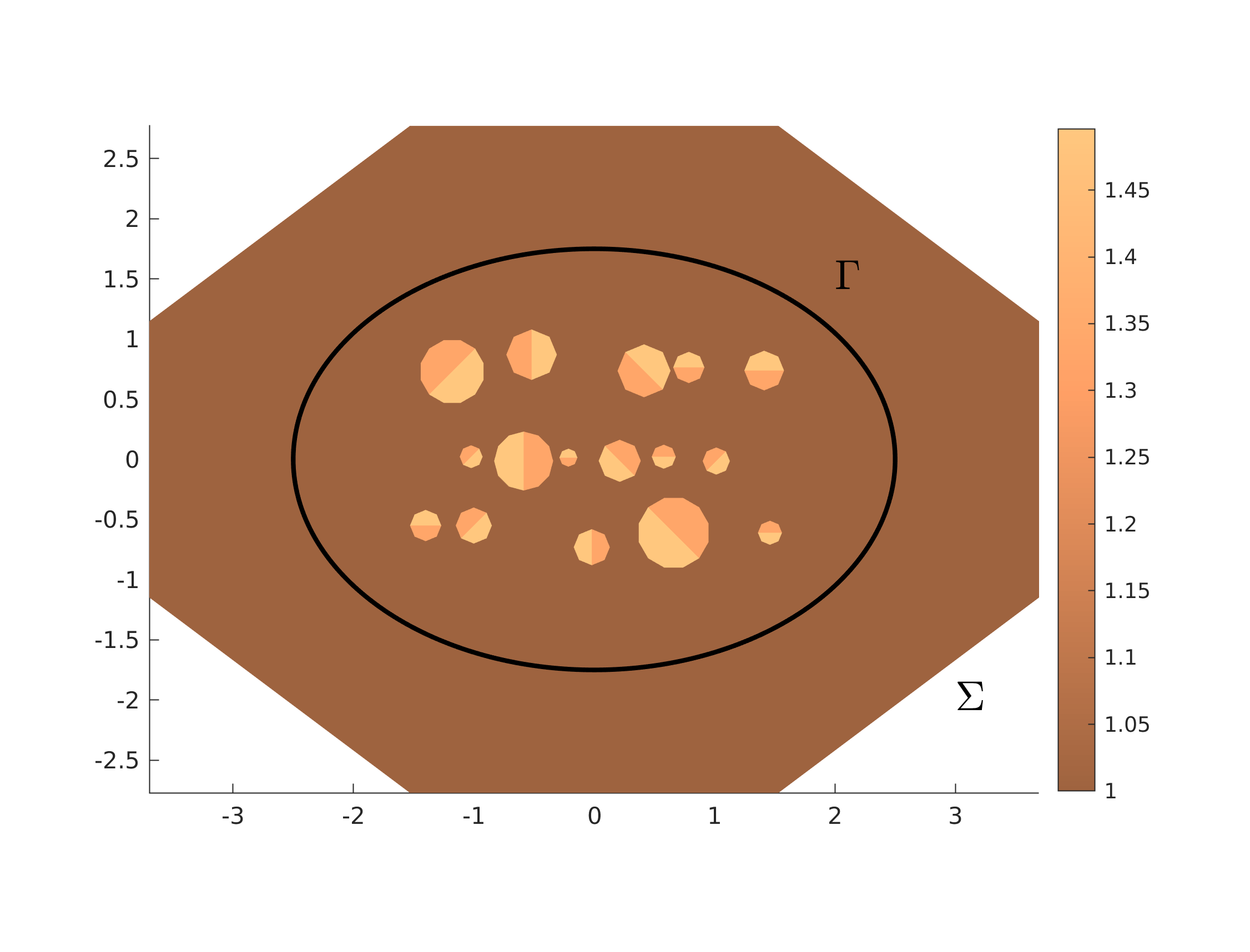
Refer to caption
Figure 3: Experiment #2 setup comprises a Janus-type configuration with 1616 Janus particles (each having a local piecewise-constant refractive index) of distinct sizes and non-smooth shapes. The FEM octagonal shaped polygonal domain Ω2\Omega_{2}, with artificial boundary Σ\Sigma, is centered at origin and has circumradius 3.5. The BEM smooth artificial boundary Γ\Gamma is an elliptical curve and the ellipse circumscribes the multi-particle heterogeneous Janus configuration.

For this set of experiments, a disconnected heterogeneous medium illustrated in Figure 3, is induced by a collection of non-smooth (polygonal) Janus particles of different sizes, and each particle is designed using two distinct materials/liquids [34]. As described in Section 1, this is a model problem for the so-called Janus configuration which has received much attention in recent years. For the Figure 3 Janus configuration based second set of numerical experiments, we used the following non-smooth (piecewise-continuous) refractive index function, defined in the full unbounded wave propagation medium, for (x,y)∈ℝ2(x,y)\in\mathbb{R}^{2}, as

n⁡(x,y)={1.333(x,y)∈ first halves of Janus particles,1.496(x,y)∈ second halves of Janus particles,1Outside the collection of Janus particles.n(x,y)=\begin{cases}1.333&\text{$(x,y)\in$ first halves of Janus particles},\\ 1.496&\text{$(x,y)\in$ second halves of Janus particles},\\ 1&\text{Outside the collection of Janus particles}.\end{cases} (5.3)

In (5.3), we recall that the numbers 1.3331.333 and 1.4961.496 correspond to, respectively, the refractive index of water and toluene at 20C; such two chemicals mix have been used in the literature to build Janus configurations [34]. Janus configuration based numerical investigations [29, 39, 38, 34, 33, 21] have been mainly restricted to simple shapes, and results in this section further demonstrate that such (shape, size, and number of particles) restrictions can be removed using efficient algorithms that can accommodate complex heterogeneous structures with efficient decomposition framework. The simulated Experiment #2 configuration with a decomposition framework is depicted in Figure 3.

For these experiments we chose medium and high frequencies with k=5,10,20k=5,10,20 (corresponding to, respectively, approximate interior problem wavelengths 8.3,16.6,33.28.3,16.6,33.2) with the coarse mesh for FEM comprising 1401 triangles. For a fixed incident plane wave case, we took the direction to be 𝒅^=(1,0)\widehat{\bm{d}}=(1,0). For simulating the OA-DSCS of the Janus configuration, we chose one thousand equally-spaced incident directions 𝒅^​(ϕ)\widehat{\bm{d}}(\phi) surrounding the configuration that corresponds to one thousand of the configuration orientations, with equally spaced orientation angles ϕ∈[0,2​π)\phi\in[0,2\pi), starting from the initial Janus configuration in Figure 3 (with ϕ=0\phi=0).

The choice of equally spaced direction angles facilitates high-order approximations to the integral in (2.4) to compute the OA-DSCS using the rectangle quadrature. We recall Remark 2.2 to highlight that our discrete FEM-BEM algorithm is efficient for computing solutions with a large number of incident waves. The first set of experiments for the Janus configuration is performed with ϕ=0\phi=0 to ensure that high-order approximations of the DSCS integrand in (2.4) can be computed using our FEM-BEM algorithm. We recall that computation of the far-field in (2.4) is a smooth post-processing of the field density on Γ\Gamma, and hence we expect that the accuracy of far-field approximations should be better, after ensuring convergence and good accuracy of the Janus configuration based FEM-BEM solution.

Our simulation results (for k=5,10,20k=5,10,20), demonstrating the FEM-BEM solution accuracy for the (ϕ=0\phi=0) Janus configuration in Figure 3, obtained using the ℙ2\mathbb{P}_{2} elements are in Table 2, and the counterpart ℙ3\mathbb{P}_{3} elements results are in Table 3. Because of the restricted regularity of the exact scattered field induced by only piecewise-continuity of the refractive index in (5.3), it can be observed from Tables 2-3, the limited (second-order) rate of convergence of the FEM solution does not improve by using ℙ3\mathbb{P}_{3} elements compared to that for ℙ2\mathbb{P}_{2} elements. However, because of the restricted regularity, it is important to use high-order ℙ3\mathbb{P}_{3} elements especially for the higher frequency (k>10k>10) cases. This is because, for example with k=20k=20 (despite using over one million FEM DoF LL), the ℙ2\mathbb{P}_{2} elements based FEM solutions with over 100%100\% errors observed in the last row of Table 2 are not acceptable, and for the same situation the ℙ3\mathbb{P}_{3} elements provide much better accurate solutions.

In Figure 5 we visualize the total field in Ω2\Omega_{2} and the scattered field in the overlapped region (ℝ2∖Ω¯1)∩Ω2(\mathbb{R}^{2}\setminus\overline{\Omega}_{1})\cap\Omega_{2}, and in Figure 5, we demonstrate the constraint of (numerically) matching the FEM and BEM solutions in the overlapped region by plotting the error in the region in log-scale. These sets of experiments illustrate the computational difficulties associated with Janus configurations based wave models, especially taking into account that linear ℙ1\mathbb{P}_{1} elements are standard for pure FEM algorithms (that do not satisfy the SRC) [24].

Further advantages of our FEM-BEM algorithm to compute high-order approximations to smooth far-fields, and hence the DSCS (with fixed incident direction angle ϕ=0\phi=0), are demonstrated in Table 4. Recall that the far-field is a smooth function defined on 𝕊1\mathbb{S}^{1}, and the uniform norm errors in the far-field were approximated by evaluating the DSCS at 14401440 equally distributed points in 𝕊1\mathbb{S}^{1}. Because of the smooth post-processing of the FEM-BEM solutions to compute far-fields, similar to the k=5k=5 results in Table 4, we observed higher accuracy for the k=10,20k=10,20 cases compared to the FEM-BEM solutions accuracy. We conclude the Experiment #2 results in Figure 6 showing the OA-DSCS as a function of the observed scattering DSCS angles (in degrees) for k=5,10,20k=5,10,20.

5,531 21,981 87,641 350,001 1,398,881
FEM BEM FEM BEM FEM BEM FEM BEM FEM BEM
020 1.6e+00 2.0e+00 3.2e-01 2.7e-01 7.8e-02 2.3e-01 1.9e-02 2.3e-01 5.2e-03 2.3e-01
040 1.6e+00 1.9e+00 3.2e-01 1.3e-01 7.8e-02 1.3e-02 1.9e-02 1.2e-03 4.7e-03 6.1e-04
080 1.6e+00 1.8e+00 3.1e-01 1.2e-01 7.7e-02 9.6e-03 1.9e-02 8.7e-04 4.7e-03 8.4e-05
160 1.6e+00 1.8e+00 3.1e-01 1.1e-01 7.7e-02 7.6e-03 1.9e-02 7.9e-04 4.7e-03 5.4e-05
5,531 21,981 87,641 350,001 1,398,881
FEM BEM FEM BEM FEM BEM FEM BEM FEM BEM
020 7.9e+01 7.8e+01 4.9e+01 4.4e+01 4.3e+01 4.0e+01 4.0e+01 4.0e+01 1.6e+01 4.0e+01
040 7.2e+01 5.5e+01 1.7e+01 1.7e+01 5.3e+00 5.7e+00 5.6e-01 5.6e-01 5.4e-01 3.8e-02
080 7.3e+01 5.5e+01 1.6e+01 1.7e+01 5.1e+00 5.4e+00 4.8e-01 4.8e-01 4.8e-01 3.2e-02
160 7.3e+01 5.6e+01 1.6e+01 1.7e+01 4.8e+00 5.1e+00 4.5e-01 4.5e-01 4.5e-01 2.8e-02
5,531 21,981 87,641 350,001 1,398,881
FEM BEM FEM BEM FEM BEM FEM BEM FEM BEM
020 6.0e+02 2.3e+02 1.5e+03 5.75e+02 1.1e+03 4.6e+02 1.6e+03 6.3e+02 1.4e+03 5.4e+02
040 4.5e+02 1.5e+02 2.8e+02 1.35e+02 3.6e+02 1.7e+02 1.3e+03 7.2e+02 1.6e+03 8.5e+02
080 3.3e+02 1.2e+02 2.3e+02 1.14e+02 4.1e+01 2.2e+01 1.2e+01 4.7e+00 1.2e+00 4.6e-01
160 3.2e+02 1.2e+02 2.4e+02 1.17e+02 4.0e+01 2.2e+01 1.2e+01 4.5e+00 1.1e+00 4.2e-01
Table 2: Experiment #2 results using ℙ2\mathbb{P}_{2} elements with k=5k=5 (top), k=10k=10 (mid), and k=20k=20 (bottom). Estimated H1−H^{1}- error for the total wave in Ω2\Omega_{2} (FEM-part) and for the scattered wave away from Γ\Gamma (BEM-part).
12,391 49,351 196,981 787,081 3,146,641
FE BEM FE BEM FE BEM FE BEM FE BEM
020 1.4e-01 3.3e-01 1.7e-02 3.1e-01 3.1e-03 3.1e-01 2.1e-03 3.1e-01 2.9e-03 3.1e-01
040 1.3e-01 9.4e-02 1.7e-02 5.2e-03 2.3e-03 8.2e-04 3.9e-04 8.0e-04 7.9e-05 8.0e-04
080 1.3e-01 7.8e-02 1.7e-02 4.2e-03 2.3e-03 2.1e-04 3.9e-04 1.1e-05 7.9e-05 1.5e-06
160 1.3e-01 7.8e-02 1.7e-02 3.7e-03 2.3e-03 2.0e-04 3.9e-04 1.2e-05 7.9e-05 1.5e-06
12,391 49,351 196,981 787,081 3,146,641
FE BEM FE BEM FE BEM FE BEM FE BEM
020 4.9e+01 5.7e+01 4.3e+01 5.2e+01 4.3e+01 5.2e+01 4.3e+01 5.2e+01 4.3e+01 5.2e+01
040 8.3e+00 1.2e+01 9.8e-01 1.3e+00 5.2e-02 5.8e-02 7.5e-03 9.6e-03 5.2e-03 8.9e-03
080 7.9e+00 1.1e+01 1.0e+00 1.4e+00 4.1e-02 3.7e-02 4.3e-03 1.3e-03 5.8e-04 7.8e-05
160 8.0e+00 1.1e+01 9.6e-01 1.3e+00 4.0e-02 3.5e-02 4.2e-03 6.5e-04 5.8e-04 5.0e-05
12,391 49,351 196,981 787,081 3,146,641
FE BEM FE BEM FE BEM FE BEM FE BEM
020 1.5e+03 6.7e+02 2.5e+03 1.2e+03 1.4e+03 6.7e+02 1.4e+03 6.5e+02 1.4e+03 6.5e+02
040 9.6e+02 5.3e+02 7.5e+02 4.1e+02 1.5e+03 1.0e+03 1.6e+03 1.1e+03 1.6e+03 1.1e+03
080 6.3e+02 3.8e+02 6.3e+01 4.1e+01 1.4e+00 6.9e-01 7.9e-02 2.5e-02 1.4e-02 6.5e-03
160 6.6e+02 3.9e+02 6.0e+02 3.9e+01 1.4e+00 7.3e-01 7.7e-02 2.4e-02 8.2e-03 9.9e-04
Table 3: Experiment #2 results using ℙ3\mathbb{P}_{3} elements with k=5k=5 (top), k=10k=10 (mid), and k=20k=20 (bottom). Estimated H1−H^{1}- error for the total wave in Ω2\Omega_{2} (FEM-part) and for the scattered wave away from Γ\Gamma (BEM-part).
Refer to captionRefer to caption
Figure 4: Experiment #2 (k=20k=20). Computed total wave (left) and scattered wave (right) using ℙ3\mathbb{P}_{3}-finite elements with 698,880698,880 elements and 1,398,8811,398,881 nodes, and using a spectral BEM with N=80N=80.
Refer to caption
Figure 5: Experiment #2 (with parameter values as in Figure 5. Absolute difference in log-scale between BEM-computed and FEM-computed approximation solutions in the overlapped region (ℝ2∖Ω¯1)∩Ω2(\mathbb{R}^{2}\setminus\overline{\Omega}_{1})\cap\Omega_{2}.
5,531 21,981 87,641 350,001 1,398,881
010 5.15e+00 4.91e+00 4.89e+00 4.89e+00 4.89e+00
020 4.37e-01 2.77e-02 3.14e-03 1.65e-03 1.33e-03
040 4.12e-01 2.53e-02 1.04e-03 2.93e-04 3.34e-05
080 4.08e-01 2.60e-02 1.58e-03 1.26e-04 2.76e-05
160 4.04e-01 2.58e-02 1.67e-03 1.39e-04 2.83e-05


NN/L{L} 12,391 49,351 196,981 787,081 3,146,641
010 4.89e+00 4.89e+00 4.89e+00 4.89e+00 4.89e+00
020 5.01e-03 1.17e-03 1.31e-03 1.36e-03 1.36e-03
040 1.03e-02 4.89e-04 2.15e-05 3.87e-07 7.79e-08
080 1.23e-02 4.47e-04 3.18e-05 7.21e-07 8.25e-08
160 1.30e-02 3.45e-04 3.88e-05 1.07e-06 4.94e-08
Table 4: Experiment #2 estimated DSCS uniform norm errors, for k=5k=5, with ℙ2\mathbb{P}_{2} (top) and ℙ3\mathbb{P}_{3} (bottom) elements and ϕ=0\phi=0 (i.e., with 𝐝=(1,0)\bm{d}=(1,0) in the incident plane wave).
Refer to caption
Figure 6: Orientation-Averaged DSCS for Experiment #2

5.3 Experiment #3 (A Baby-Yoda shaped heterogeneous region)

In this set of experiments, we demonstrate flexibility of our FEM-BEM algorithm with complex structured heterogeneous regions. To this end, we consider a Baby-Yoda like domain, depicted in Figure 7 on which the refraction index function is defined. The function is taken to be piecewise-constant at distinct parts of the domain with values indicated in Figure 7, leading to the total field solution uu with limited regularity. In Figure 7 we also show the curve Γ\Gamma taken for our BEM computations, which is similar to the smooth curve in Experiment #1 with some rescaling; and the choice of Σ\Sigma is such that the FEM computational domain Ω2\Omega_{2} is a rectangle. Similar to the first two sets of experiments, we simulate the model with wavenumbers k=5,10,20k=5,10,20, and for the configuration in Figure 7 these values respectively correspond to 9.2,18.4,36.89.2,18.4,36.8 interior wavelengths region Ω2\Omega_{2}.

Refer to caption
Figure 7: Experiment #3 setup with Baby-Yoda heterogeneous region.

Similar to the first two sets of experiments, sample results in Table 5 demonstrate the power of our overlapped FEM-BEM algorithm even for the case of simulation of non-smooth wave fields induced by only piecewise-continuous refractive index in complicated heterogeneous regions. Another marked advantage of our FEM-BEM algorithm is the low number of iterations required for convergence of the GMRES to iteratively solve the resulting interface algebraic linear systems (3.13a). In particular, as can be observed in Table 6, for each fixed wavenumber kk the number of required GMRES iterations is independent of the numbers of FEM-BEM DoFs (level of discretizations). In addition, even as the frequency is doubled the required iterations grow only mildly (to achieve a fixed error tolerance), and because of the well-conditioning the interface system  (3.13a), even for the high-frequency case, less than 100100 GMRES iterations are required without using any preconditioner. We conclude the numerical experiments section with visualizations in Figure 9 for (i) the total field in Ω2\Omega_{2}; (ii) the scattered field in the overlapped region Ω12=(ℝ2∖Ω¯1)∩Ω2\Omega_{12}=(\mathbb{R}^{2}\setminus\overline{\Omega}_{1})\cap\Omega_{2}; and (iii) accurate matching of the FEM and BEM solutions in the overlapped region in Figure 9.

114,094 455,785 1,821,961
FE BEM FE BEM FE BEM
020 3.1e-02 3.0e-01 2.0e-02 3.0e-01 1.6e-02 3.0e-01
040 2.7e-02 2.2e-03 1.4e-02 2.0e-03 6.2e-03 2.0e-03
080 2.7e-02 9.6e-04 1.4e-02 2.4e-04 6.2e-03 5.2e-05
160 2.7e-02 9.5e-04 1.4e-02 2.4e-04 6.2e-03 5.2e-05
114,094 455,785 1,821,961
FE BEM FE BEM FE BEM
020 2.1e+01 1.9e+01 2.1e+01 1.9e+01 2.1e+01 1.9e+01
040 8.5e-02 2.8e-02 2.9e-02 5.7e-02 1.3e-02 5.1e-03
080 8.5e-02 2.7e-02 2.9e-02 2.1e-03 1.3e-02 2.1e-04
160 8.5e-02 2.6e-02 2.9e-02 2.0e-03 1.3e-02 2.1e-04
114,094 455,785 1,821,961
FE BEM FE BEM FE BEM
020 1.7e+02 1.1e+02 1.7e+02 1.1e+02 1.7e+02 1.1e+02
040 5.1e+00 4.3e+00 5.0e+01 4.4e+00 5.0e+01 4.4e+00
080 1.0e+00 2.7e-01 1.3e-01 6.5e-03 3.0e-02 8.8e-04
160 1.0e+00 2.7e-01 1.3e-01 6.2e-03 3.0e-02 8.6e-04
Table 5: Experiment #3 results using ℙ3\mathbb{P}_{3} elements with k=5k=5 (top), k=10k=10 (mid), and k=20k=20 (bottom). Estimated H1−H^{1}- error for the total wave in Ω2\Omega_{2} (FEM-part) and for the scattered wave away from Γ\Gamma (BEM-part).
48,137 192,153 767,825 3,069,729
k=5 k=10 k=20 k=5 k=10 k=20 k=5 k=10 k=20 k=5 k=10 k=20
020 22 38 40 22 38 40 22 38 040 22 38 40
040 22 38 67 22 38 67 22 38 067 22 38 67
080 22 38 67 22 38 67 22 38 067 22 38 67
160 22 38 67 22 38 67 22 38 067 22 38 67
114,094 455,785 1,821,961
k=5 k=10 k=20 k=5 k=10 k=20 k=5 k=10 k=20
020 22 38 40 22 38 40 22 38 40
040 22 38 67 22 38 67 22 38 67
080 22 38 67 22 38 67 22 38 67
160 22 38 67 22 38 67 22 38 67
Table 6: Experiment #3. Total number of GMRES iterations for convergence (with tolerance 10−810^{-8}) using ℙ2\mathbb{P}_{2} (top) and ℙ3\mathbb{P}_{3} (bottom) elements. For each fixed kk, the total number of required GMRES iterations is independent of NN and LL and grows mildly with respect to increase in the wavenumber kk.
Refer to captionRefer to caption
Figure 8: Experiment #3 (k=20k=20). Computed total wave (left) and scattered wave (right) using ℙ3\mathbb{P}_{3}-finite elements with 478,464478,464 elements and 1,821,9611,821,961 nodes, and using a spectral BEM with N=80N=80.
Refer to caption
Figure 9: Experiment #3 (with parameter values as in Figure 9. Absolute difference in log-scale between BEM-computed and FEM-computed approximation solutions in the overlapped region Ω12=(ℝ2∖Ω¯1)∩Ω2\Omega_{12}=(\mathbb{R}^{2}\setminus\overline{\Omega}_{1})\cap\Omega_{2}.

Acknowledgement

We sincerely thank the anonymous referees for suggestions which helped to improve the paper. The first author (Domínguez) is supported by the project MTM2017-83490-P. The second author (Ganesh) gratefully acknowledges the support of the Simons Foundation.

References

  • [1] R.A. Adams and J.J.F. Fournier. Sobolev spaces, volume 140 of Pure and Applied Mathematics (Amsterdam). Elsevier/Academic Press, Amsterdam, second edition, 2003.
  • [2] S. Bertoluzza. The discrete commutator property of approximation spaces. C. R. Acad. Sci. Paris Sér. I Math., 329(12):1097–1102, 1999.
  • [3] H. Brakhage and P. Werner. Über das Dirichletsche Aussenraumproblem für die Helmholtzsche Schwingungsgleichung. Arch. Math., 16:325–329, 1965.
  • [4] S.C. Brenner and L.R. Scott. The mathematical theory of finite element methods, volume 15 of Texts in Applied Mathematics. Springer, New York, third edition, 2008.
  • [5] P.G. Ciarlet. The Finite Element Method for Elliptic Problems. Classics in Applied Mathematics. Society for Industrial and Applied Mathematics, 2002.
  • [6] D. Colton and R. Kress. Inverse Acoustic and Electromagnetic Scattering Theory. Springer, 4th edition, 2019.
  • [7] M. Costabel. Boundary integral operators on Lipschitz domains: elementary results. SIAM J. Math. Anal., 19(3):613–626, 1988.
  • [8] J. Coyle and P. Monk. Scattering of time-harmonic electromagnetic waves by anisotropic in homogeneous scatterers or impenetrable obstacles. SIAM J. Math. Anal., 37:1590–1617, 2004.
  • [9] P. G. de Gennes. Soft Matter (Nobel Lecture). Angew. Chem. Int. Ed. Engl., 31:842–845, 1992.
  • [10] V. Domínguez, M. Ganesh, and F.J. Sayas. An overlapping decomposition framework for wave propagation in heterogeneous and unbounded media: Formulation, analysis, algorithm, and simulation. J. Comput. Phys., 403:109052, 2020.
  • [11] V. Domínguez and F.-J. Sayas. Stability of discrete liftings. C. R. Math. Acad. Sci. Paris, 337(12):805–808, 2003.
  • [12] V. Domínguez and C. Turc. High order Nyström methods for transmission problems for Helmholtz equations. In Trends in differential equations and applications, volume 8 of SEMA SIMAI Springer Ser., pages 261–285. Springer, [Cham], 2016.
  • [13] M. Ganesh and S. C. Hawkins. Algorithm 975: TMATROM—a T-matrix reduced order model software. ACM Trans. Math. Softw., 44:9:1–9:18, 2017.
  • [14] M. Ganesh, S. C. Hawkins, and R. Hiptmair. Convergence analysis with parameter estimates for a reduced basis acoustic scattering T-matrix method. IMA J. Numer. Anal., 32:1348–1374, 2012.
  • [15] M. Ganesh and C. Morgenstern. High-order FEM-BEM computer models for wave propagation in unbounded and heterogeneous media: application to time-harmonic acoustic horn problem. J. Comput. Appl. Math., 307:183–203, 2016.
  • [16] M. Ganesh and C. Morgenstern. High-order FEM domain decomposition models for high-frequency wave propagation in heterogeneous media. Comp. Math. Appl. (CAMWA), 75:1961–1972, 2018.
  • [17] M. Ganesh and C. Morgenstern. A coercive heterogeneous media Helmholtz model: formulation, wavenumber-explicit analysis, and preconditioned high-order FEM. Numerical Algorithms, 83:1441–1487, 2020.
  • [18] C. Geuzaine and J.-F. Remacle. Gmsh: A 3-D finite element mesh generator with built-in pre- and post-processing facilities. International Journal for Numerical Methods in Engineering, 79:1309 – 1331, 2009.
  • [19] A. Gillman, A. H. Barnett, and P.-G. Martinsson. A spectrally accurate direct solution technique for frequency-domain scattering problems with variable media. BIT Numerical Mathematics, 55(1):141–170, 2015.
  • [20] P. Grisvard. Elliptic problems in nonsmooth domains, volume 69 of Classics in Applied Mathematics. Society for Industrial and Applied Mathematics (SIAM), Philadelphia, PA, 2011.
  • [21] S. C. Hawkins, T. Rother, and J. Wauer. Numerical study of acoustic scattering by Janus spheres. J. Acoust. Soc. Am., 147:4097, 2020.
  • [22] C. Hazard and M. Lenoir. On the solutions of time-harmonic scattering problems for maxwell’s equations. SIAM J. Math. Anal., 27:1597–1630, 1996.
  • [23] G. C. Hsiao and W. L. Wendland. Boundary integral equations, volume 164 of Applied Mathematical Sciences. Springer-Verlag, Berlin, 2008.
  • [24] F. Ihlenburg. Finite element analysis of acoustic scattering, volume 132 of Applied Mathematical Sciences. Springer-Verlag, New York, 1998.
  • [25] A. Jami and M. Lenoir. A variational formulation for exterior problems in linear hydrodynamics. Comput. Methods Appl. Mech. Engrg., 16:341–359, 1978.
  • [26] A. Kirsch and P. Monk. Convergence analysis of a coupled finite element and spectral method in acoustic scattering. IMA J. Numer. Anal., 10(3):425–447, 1990.
  • [27] A. Kirsch and P. Monk. An analysis of the coupling of finite-element and Nyström methods in acoustic scattering. IMA J. Numer. Anal., 14(4):523–544, 1994.
  • [28] R. Kress. Linear integral equations, volume 82 of Applied Mathematical Sciences. Springer, New York, third edition, 2014.
  • [29] M. Lattuada and A. Hatton. Synthesis, properties and applications of janus nanoparticles. Nano Today, 6:286–308, 2011.
  • [30] W. McLean. Strongly elliptic systems and boundary integral equations. Cambridge University Press, Cambridge, 2000.
  • [31] J.-C. Nédélec. Acoustic and electromagnetic equations, volume 144 of Applied Mathematical Sciences. Springer-Verlag, New York, 2001. Integral representations for harmonic problems.
  • [32] J. A. Nitsche and A. H. Schatz. Interior estimates for Ritz-Galerkin methods. Math. Comp., 28:937–958, 1974.
  • [33] T. Rother. Sound Scattering on Spherical Objects. Springer, New York, 2020.
  • [34] T. M. Ruhland, A. H. Gröschel, N. Ballard, T. S. Skelhon, A.Walther, A. H. E. Müller, and S. A. F. Bon. Influence of Janus particle shape on their interfacial behavior at liquid-liquid interfaces. Langmuir, 29:1388–1394, 2013.
  • [35] J. Saranen and G. Vainikko. Periodic integral and pseudodifferential equations with numerical approximation. Springer Monographs in Mathematics. Springer-Verlag, Berlin, 2002.
  • [36] F. J. Sayas. The validity of Johnson-Nédélec’s BEM-FEM coupling on polygonal interfaces. SIAM Review, 55:131–146, 2013.
  • [37] L.R. Scott and S. Zhang. Finite element interpolation of nonsmooth functions satisfying boundary conditions. Math. Comp., 54(190):483–493, 1990.
  • [38] M. Vafaeezadeh and W. R. Thiel. Janus interphase catalysts for interfacial organic reactions. J. Mol. Liq., 315:113735, 2020.
  • [39] J. Zhang, A. Gryzbowski, and Granick. Janus particle synthesis, assembly and application. Langmuir, 33:6964–6977, 2017.

Appendix A Sobolev convergence estimates for some projections

In this section we collect some useful results for projections on finite element spaces. The first set of results is concerned with finite element spaces on polygonal compact closed boundaries in ℝ2\mathbb{R}^{2}. There finite element spaces are inherited by taking Dirichlet trace of finite element spaces on triangular meshes. We finish this section proving a commutation property for Scott-Zhang type projections, which is required in Appendix B for deriving superconvergence results of the finite element solution in stronger norms that are also valid in three dimensions. We think that most of the described results here belong to the folklore in finite element analysis. We include results below for the sake of completeness.

A.1 Projections on polygonal boundary finite element spaces

Let Σ\Sigma be a polygonal simply connected closed curve with interior Ω⊂ℝ2\Omega\subset\mathbb{R}^{2}. We consider {𝒯h}h≥0\{{\cal T}_{h}\}_{h\geq 0} a sequence of regular triangular meshes of Ω\Omega and denote by {τh}h≥0\{\tau_{h}\}_{h\geq 0} that inherited on Σ\Sigma. Without loss of generality we can assume that hΣ≈hh_{\Sigma}\approx h, where hΣh_{\Sigma} and hh are the maximum, respectively, of the diameters of the elements of the grids 𝒯h{\cal T}_{h} and τh{\tau}_{h}. In addition, let

ℙh,d:={uh∈𝒞0​(Ω):uh|Th∈ℙd},γΣ​ℙh,d\mathbb{P}_{h,d}:=\{{u}_{h}\in{\cal C}^{0}(\Omega):\ u_{h}|_{T_{h}}\in\mathbb{P}_{d}\},\qquad\gamma_{\Sigma}\mathbb{P}_{h,d}

denote the space of continuous finite elements space in Ω\Omega and its boundary Σ\Sigma. We denote by

Qh:𝒞⁡(Ω)→ℙh,d,QΣh:𝒞⁡(Σ)→γΣ​ℙh,d\mathrm{Q}_{h}:{\cal C}(\Omega)\to\mathbb{P}_{h,d},\qquad{\rm Q}^{h}_{\Sigma}:{\cal C}(\Sigma)\to\gamma_{\Sigma}\mathbb{P}_{h,d}

the corresponding nodal (Lagrange) interpolation operators. Note that

γΣ​Qh​uh=QΣh​γΣ​uh,∀uh∈ℙh,d.\gamma_{\Sigma}\mathrm{Q}_{h}u_{h}={\rm Q}^{h}_{\Sigma}\gamma_{\Sigma}u_{h},\quad\forall u_{h}\in\mathbb{P}_{h,d}.

Our objectives in this section are twofold: (a) derive convergence estimates in the Sobolev norms ∥⋅∥Hs​(Σ)\|\cdot\|_{H^{s}(\Sigma)} for QΣh{\rm Q}^{h}_{\Sigma} and s≥0s\geq 0 (see (2.5) for the definition we have taken for these spaces for s>1s>1); (b) define an alternative stable and convergent projection in weaker norms. In particular, we are interested in working with functions H1/2​(Σ)H^{1/2}(\Sigma), the trace space, for which the interpolant cannot be defined since the space contains discontinuous functions. Next, we start with the first objective:

Proposition A.1.

For any s∈[0,1]s\in[0,1] and s≤t<d+1s\leq t<d+1 with t>1/2t>1/2 there exists C>0C>0 such that

‖QΣh​fΣ−fΣ‖Hs​(Σ)≤C​hΣt−s​‖f‖Ht​(Σ).\|{\rm Q}^{h}_{\Sigma}f_{\Sigma}-f_{\Sigma}\|_{H^{s}(\Sigma)}\leq Ch_{\Sigma}^{t-s}\|f\|_{H^{t}(\Sigma)}. (A.1)

Furthermore, for any t>d+1t>d+1

‖QΣh​fΣ−fΣ‖Hs​(Σ)≤C​hΣd+1−s​‖f‖Ht​(Σ)\|{\rm Q}^{h}_{\Sigma}f_{\Sigma}-f_{\Sigma}\|_{H^{s}(\Sigma)}\leq Ch_{\Sigma}^{d+1-s}\|f\|_{H^{t}(\Sigma)} (A.2)

with C>0C>0 depending only on s∈[0,1]s\in[0,1] and tt.

Proof.

We start with a classical result: for s∈{0,1}s\in\{0,1\} and t>max⁡{1/2,s}t>\max\{1/2,s\} [5, Th. 3.1.6]

‖QΣh​fΣ−fΣ‖Hs​(Σ)≤C′​hΣt−s​‖fΣ‖ℋt​(Σ)\|{\rm Q}^{h}_{\Sigma}f_{\Sigma}-f_{\Sigma}\|_{H^{s}(\Sigma)}\leq C^{\prime}h_{\Sigma}^{t-s}\|f_{\Sigma}\|_{{\cal H}^{t}(\Sigma)}

where {Σℓ}ℓ\{\Sigma_{\ell}\}_{\ell} are the edges of Σ\Sigma and Ht​(Σℓ)H^{t}(\Sigma_{\ell}) the corresponding classical Sobolev space, and

‖fΣ‖ℋt​(Σ)2:=∑ℓ‖fΣ‖Ht​(Σℓ)2.\|f_{\Sigma}\|_{{\cal H}^{t}(\Sigma)}^{2}:=\sum_{\ell}\|f_{\Sigma}\|^{2}_{H^{t}(\Sigma_{\ell})}.

For t>0t>0, with t≠1,2,…,t\neq 1,2,\ldots, we then use that the trace operator is also continuous in this norm

‖γΣ​u‖ℋt​(Σ)≤C​‖u‖Ht+1/2​(Ω),∀u∈Ht+1/2​(Ω)\|\gamma_{\Sigma}u\|_{{\cal H}^{t}(\Sigma)}\leq C\|u\|_{H^{t+1/2}(\Omega)},\quad\forall u\in H^{t+1/2}(\Omega) (A.3)

cf. [20, Th. 1.5.2.8] (the bound in (A.3) breaks precisely for t=0,1,2​…t=0,1,2\ldots; see also [23, Th. 4.2.7]) which proves (A.1) for the considered non-integer values of tt. By interpolation of Sobolev spaces, we can extend the result for any t<d+1t<d+1 and s∈[0,1]s\in[0,1], and hence (A.1) holds.

The bound (A.2) can be proven by starting from

‖QΣh​fΣ−fΣ‖Hs​(Σ)≤C​hΣd+1−s​‖fΣ‖ℋd+1+ε​(Σ),\|{\rm Q}^{h}_{\Sigma}f_{\Sigma}-f_{\Sigma}\|_{H^{s}(\Sigma)}\leq Ch_{\Sigma}^{d+1-s}\|f_{\Sigma}\|_{{\cal H}^{d+1+\varepsilon}(\Sigma)},

with ε∈(0,1)\varepsilon\in(0,1) and again using (A.3). ∎

We will focus next on constructing a projection PΣh:H1/2​(Σ)→γΣ​ℙh,d{\rm P}_{\Sigma}^{h}:H^{1/2}(\Sigma)\to\gamma_{\Sigma}\mathbb{P}_{h,d} with same convergence rates in an extended Sobolev scale. A key fact in this construction is the existence of a Scott-Zhang-type projection cf. [37] (see also [11]). Specifically, there exists a continuous linear mapping Πh,d:Hs​(Ω)→ℙh,d\Pi_{h,d}:H^{s}(\Omega)\to\mathbb{P}_{h,d}, with s>1/2s>{1/2}, satisfying

  1. 1.

    Πh\Pi_{h} is a projection:

    Πh​vh=vh,∀vh∈ℙh,d.\Pi_{h}v_{h}=v_{h},\quad\forall v_{h}\in\mathbb{P}_{h,d}. (A.4a)
  2. 2.

    The image of any element with null trace has null trace as well:

    γΣ​Πh​v=0,ifγΣ​v=0.\gamma_{\Sigma}\Pi_{h}v=0,\quad\text{if}\quad\gamma_{\Sigma}v=0. (A.4b)
  3. 3.

    It is quasi-local: for any triangle K∈𝒯hK\in{\cal T}_{h},

    Πh​v|T=0,ifv|ST=0, with ​ST:=⋃T¯′∩T¯≠∅T′∈𝒯hT¯′.\Pi_{h}v|_{T}=0,\quad\text{if}\quad v|_{S_{T}}=0,\text{ with }S_{T}:=\bigcup_{\stackrel{{\scriptstyle T^{\prime}\in{\cal T}_{h}}}{{\overline{T}^{\prime}\cap\overline{T}\neq\emptyset}}}\overline{T}^{\prime}. (A.4c)

    Furthermore, for any 0≤s≤t0\leq s\leq t with s∈[0,3/2)s\in[0,3/2) and 1/2<t≤d+11/2<t\leq d+1 there exists C=C⁡(s,t)C=C(s,t) so that

    ‖Πh​v−v‖Hs​(T)≤C​hTt−s​‖v‖Ht​(ST).\|\Pi_{h}v-v\|_{H^{s}(T)}\leq Ch_{T}^{t-s}\|v\|_{H^{t}(S_{T})}. (A.4d)

    The constant C⁡(s,t)C(s,t) depends only on the chunkiness parameter of the grid. As consequence of (A.4d) we have

    [∑T∈𝒯hhT2​(s−t)​‖Πh​v−v‖Hs​(T)2]1/2≤C​‖v‖Ht​(Ω).\left[\sum_{T\in{\cal T}_{h}}h_{T}^{2(s-t)}\|\Pi_{h}v-v\|^{2}_{H^{s}(T)}\right]^{1/2}\leq C\|v\|_{H^{t}(\Omega)}. (A.4e)

Since for s∈[0,1/2)∪[1,3/2)s\in[0,1/2)\cup[1,3/2), we have

‖v‖Hs​(Ω)≤C​[∑T∈𝒯h‖v‖Hs​(T)2]1/2,\|v\|_{H^{s}(\Omega)}\leq C\left[\sum_{T\in{\cal T}_{h}}\|v\|^{2}_{H^{s}(T)}\right]^{1/2}, (A.5)

the simpler estimate

‖Πh​v−v‖Hs​(Ω)≤C​ht−s​‖v‖Ht​(Ω).\|\Pi_{h}v-v\|_{H^{s}(\Omega)}\leq Ch^{t-s}\|v\|_{H^{t}(\Omega)}. (A.6)

can be derived from (A.4d), first for s∈[0,1/2)∪[1,3/2)s\in[0,1/2)\cup[1,3/2), and then can be extended for s∈[1/2,1)s\in[1/2,1) by interpolation of Sobolev spaces.

Remark A.2.

The proof of (A.5) is based on working with the Slobodeckij form of the Sobolev norm: for non-integer s>0s>0 and for any Lipschitz domain D⊂ℝmD\subset\mathbb{R}^{m}

‖u‖Hs​(D)2=‖u‖Hs¯​(D)2+∑|𝜶|=s¯∫D∫D|∂𝜶u⁡(𝒙)−∂𝜶u⁡(𝒚)||𝒙−𝒚|m+2​(s−s¯)​𝑑𝒙​𝑑𝒚,\|u\|_{H^{s}(D)}^{2}=\|u\|_{H^{\underline{s}}(D)}^{2}+\sum_{|\bm{\alpha}|=\underline{s}}\int_{D}\int_{D}\frac{|\partial_{\bm{\alpha}}u(\bm{x})-\partial_{\bm{\alpha}}u(\bm{y})|}{|{\bm{x}}-{\bm{y}}|^{m+2({s}-\underline{s})}}{\rm d}\bm{x}\,{\rm d}{\bm{y}},

where s¯\underline{s} is the largest integer less than ss. Then, for t∈(0,1/2)t\in(0,1/2), it is easy to derive the estimate

‖v‖Ht​(Ω)2≤Ct,Ω​[∑T∈𝒯h‖v‖Ht​(T)2+∫T|v⁡(𝒙)|2ρ​(𝒙,∂T)2​t​𝑑𝒙]\|v\|^{2}_{H^{t}(\Omega)}\leq C_{t,\Omega}\left[\sum_{T\in{\cal T}_{h}}\|v\|^{2}_{H^{t}(T)}+\int_{T}\frac{|v(\bm{x})|^{2}}{\rho(\bm{x},\partial T)^{2t}}\,{\rm d}\bm{x}\right]

where

ρ⁡(𝒙,∂T)=inf𝒚∈∂T|𝒙−𝒚|.\rho({\bm{x}},\partial T)=\inf_{\bm{y}\in\partial T}|{\bm{x}}-{\bm{y}}|.

A Hardy-type inequality (see [30, Lemma 3.32]) allows to bound the above integral term by

∫T|v⁡(𝒙)|2ρ​(𝒙,∂T)2​t​𝑑𝒙≤C​‖v‖Ht​(T)2.\int_{T}\frac{|v(\bm{x})|^{2}}{\rho(\bm{x},\partial T)^{2t}}\,{\rm d}\bm{x}\leq C\|v\|^{2}_{H^{t}(T)}.

The constant CC appearing above depends on tt and on the chunkiness parameter of TT. This inequality does not hold for t∈[1/2,1)t\in[1/2,1) since the last integral in the left hand side is expected to be non-convergent. The result for t>1t>1 is a simple extension of this argument.

The last ingredient is a right inverse of the trace operator RΣ​Ω:Hs​(Σ)→Hs+1/2​(Ω){\rm R}_{\Sigma\Omega}:H^{s}(\Sigma)\to H^{s+1/2}(\Omega) for s∈(0,1]s\in(0,1] . For instance, one can take

RΣ​ΩgΣ:=u,with u satisfying Δu=0,γΣ​u=gΣ,{\rm R}_{\Sigma\Omega}g_{\Sigma}:=u,\quad\text{with $u$ satisfying }\Delta u=0,\quad\text{$\gamma_{\Sigma}u=g_{\Sigma}$},

the Dirichlet solution for the Laplace operator. Such operator is continuous, not only for s∈(0,1)s\in(0,1), but it attains the end point s=1s=1 as well (cf. [30, Chapter 6]; see Theorem 6.12 and the discussion following it).

We are ready to define the desired projection on the finite element space on the boundary γΣ​ℙh,d\gamma_{\Sigma}\mathbb{P}_{h,d}. To this end, we first set

PΣh:=γΣ​Πh​RΣ​Ω.{\rm P}_{\Sigma}^{h}:=\gamma_{\Sigma}\Pi_{h}{\rm R}_{\Sigma\Omega}.
Proposition A.3.

Let PΣh:Hs​(Σ)→γΣ​ℙh,d{\rm P}_{\Sigma}^{h}:H^{s}(\Sigma)\to\gamma_{\Sigma}\mathbb{P}_{h,d} as above. Then

‖PΣh​fΣ−fΣ‖Hs​(Σ)≤C​hΣt−s​‖fΣ‖Ht​(Σ),0≤s<1,s≤t<d+1,t>0,\|{\rm P}_{\Sigma}^{h}f_{\Sigma}-f_{\Sigma}\|_{H^{s}(\Sigma)}\leq Ch_{\Sigma}^{t-s}\|f_{\Sigma}\|_{H^{t}(\Sigma)},\quad 0\leq s<1,\quad s\leq t<d+1,\quad t>0, (A.7)

where CC is independent of fΣf_{\Sigma} and hh. Furthermore, for any s∈[0,1)s\in[0,1) and t>d+1t>d+1, there exists C>0C>0 such that

‖PΣh​fΣ−fΣ‖Hs​(Σ)≤C​hΣd+1−s​‖f‖Ht​(Σ).\|{\rm P}^{h}_{\Sigma}f_{\Sigma}-f_{\Sigma}\|_{H^{s}(\Sigma)}\leq Ch_{\Sigma}^{d+1-s}\|f\|_{H^{t}(\Sigma)}. (A.8)
Proof.

By construction, Πh\Pi_{h} is a projection. Indeed, if Qh:𝒞⁡(Ω)→ℙh,d{\rm Q}_{h}:{\cal C}(\Omega)\to\mathbb{P}_{h,d} is the nodal d−d-Lagrange interpolation operator, and since γΣ​Qh=QΣh​γΣ\gamma_{\Sigma}{\rm Q}_{h}={\rm Q}^{h}_{\Sigma}\gamma_{\Sigma}, we have that

γΣ​Πh​RΣ​Ω​fΣh−fΣh\displaystyle\gamma_{\Sigma}\Pi_{h}{\rm R}_{\Sigma\Omega}f_{\Sigma}^{h}-f_{\Sigma}^{h} =\displaystyle= γΣ​(Πh−Qh)​RΣ​Ω​fΣh=γΣ​Πh​(I−Qh)​RΣ​Ω​fΣh⏟∈H01​(Ω)=0\displaystyle\gamma_{\Sigma}(\Pi_{h}-{\rm Q}_{h}){\rm R}_{\Sigma\Omega}f_{\Sigma}^{h}=\gamma_{\Sigma}\Pi_{h}\underbrace{({\rm I}-{\rm Q}_{h}){\rm R}_{\Sigma\Omega}f_{\Sigma}^{h}}_{\in H_{0}^{1}(\Omega)}=0

by (A.4b).

On the other hand, for t∈(1/2,1]t\in(1/2,1] with t≥st\geq s, and s∈(0,1)s\in(0,1), and by the continuity of the trace operator,

‖PΣh​fΣ−fΣ‖Hs​(Σ)\displaystyle\|{\rm P}_{\Sigma}^{h}f_{\Sigma}-f_{\Sigma}\|_{H^{s}(\Sigma)} ≤\displaystyle\leq C​‖Πh​RΣ​Ω​fΣ−RΣ​Ω​fΣ‖Hs+1/2​(Ω)\displaystyle C\|\Pi_{h}{\rm R}_{\Sigma\Omega}f_{\Sigma}-{\rm R}_{\Sigma\Omega}f_{\Sigma}\|_{H^{s+1/2}(\Omega)} (A.9)
≤\displaystyle\leq C′​hΣt−s​‖RΩ​Σ​fΣ‖Ht+1/2​(Ω)≤C′′​hΣt−s​‖fΣ‖Ht​(Σ).\displaystyle C^{\prime}h_{\Sigma}^{t-s}\|{\rm R}_{\Omega\Sigma}f_{\Sigma}\|_{H^{t+1/2}(\Omega)}\leq C^{\prime\prime}h_{\Sigma}^{t-s}\|f_{\Sigma}\|_{H^{t}(\Sigma)}.

To prove the estimate in H0​(Σ)=L2​(Σ)H^{0}(\Sigma)=L^{2}(\Sigma) we recall the trace inequality cf [4, Th. 1.6.6]

‖γΣ​u‖L2​(Σ)2≤C⁡(‖u‖L2​(Ω)2+‖u‖L2​(Ω)​‖u‖H1​(Ω))≤C⁡(1+12​hΣ−1)​‖u‖L2​(Ω)2+12​C​hΣ​‖u‖H1​(Ω)2\|\gamma_{\Sigma}u\|_{L^{2}(\Sigma)}^{2}\leq C\big(\|u\|_{L^{2}(\Omega)}^{2}+\|u\|_{L^{2}(\Omega)}\|u\|_{H^{1}(\Omega)}\big)\leq C(1+\tfrac{1}{2}h_{\Sigma}^{-1})\|u\|_{L^{2}(\Omega)}^{2}+\tfrac{1}{2}Ch_{\Sigma}\|u\|^{2}_{H^{1}(\Omega)}

which yields

‖PΣh​fΣ−fΣ‖L2​(Σ)\displaystyle\|{\rm P}_{\Sigma}^{h}f_{\Sigma}-f_{\Sigma}\|_{L^{2}(\Sigma)} ≤\displaystyle\leq ChΣ1/2∥ΠhRΩ​ΣfΣ−RΩ​ΣfΣ∥H1​(Ω)+ChΣ−1/2∥ΠhRΩ​ΣfΣ−RΩ​ΣfΣ∥H0​(Ω)\displaystyle Ch_{\Sigma}^{1/2}\|\Pi_{h}{\rm R}_{\Omega\Sigma}f_{\Sigma}-{\rm R}_{\Omega\Sigma}f_{\Sigma}\|_{H^{1}(\Omega)}+Ch_{\Sigma}^{-1/2}\|\Pi_{h}{\rm R}_{\Omega\Sigma}f_{\Sigma}-{\rm R}_{\Omega\Sigma}f_{\Sigma}\|_{H^{0}(\Omega)}
≤\displaystyle\leq C′​hΣt​‖RΩ​Σ​fΣ‖Ht+1/2​(Ω)≤C′​hΣt​‖fΣ‖Ht​(Σ).\displaystyle C^{\prime}h_{\Sigma}^{t}\|{\rm R}_{\Omega\Sigma}f_{\Sigma}\|_{H^{t+1/2}(\Omega)}\leq C^{\prime}h^{t}_{\Sigma}\|f_{\Sigma}\|_{H^{t}(\Sigma)}.

We have then proved (A.7) for 0≤s<10\leq s<1 and max⁡{s,1/2}<t≤1\max\{s,1/2\}<t\leq 1 and therefore it only remains to extend this result for t>1t>1. But,

‖PΣh​fΣ−fΣ‖Hs​(Σ)\displaystyle\|{\rm P}_{\Sigma}^{h}f_{\Sigma}-f_{\Sigma}\|_{H^{s}(\Sigma)} =\displaystyle= ‖PΣh​(fΣ−QΣh​f)−(fΣ−QΣh​f)‖Hs​(Σ)≤C​hΣ1−s​‖fΣ−QΣh​fΣ‖H1​(Σ)\displaystyle\|{\rm P}_{\Sigma}^{h}(f_{\Sigma}-{\rm Q}_{\Sigma}^{h}f)-(f_{\Sigma}-{\rm Q}_{\Sigma}^{h}f)\|_{H^{s}(\Sigma)}\leq Ch_{\Sigma}^{1-s}\|f_{\Sigma}-{\rm Q}_{\Sigma}^{h}f_{\Sigma}\|_{H^{1}(\Sigma)}

and the result follows from Proposition A.1.

∎

Note that, using the above arguments, (A.7) cannot be extended to s=1s=1.

A.2 Commutator properties for Scott-Zhang projections

We end this section showing a commutation property for Πh\Pi_{h}. We stress out that the result is also valid in 3D for tetrahedral meshes with minor but direct modifications.

Lemma A.4.

For any ϖ∈𝒞∞​(Ω)\varpi\in{\cal C}^{\infty}(\Omega) there exists C>0C>0 so that for d≥2d\geq 2 and s∈[0,3/2)s\in[0,3/2)

‖Πh​(ϖ​wh)−ϖ​wh‖Hs​(Ω)≤C​h​‖wh‖Hs​(Ω),∀wh∈ℙh,d.\|\Pi_{h}(\varpi w_{h})-\varpi w_{h}\|_{H^{s}(\Omega)}\leq Ch\|w_{h}\|_{H^{s}(\Omega)},\quad\forall w_{h}\in\mathbb{P}_{h,d}.

For d=1d=1 (linear finite elements), we have instead

‖Πh​(ϖ​wh)−ϖ​wh‖Hs​(Ω)≤C​hmin⁡{1,2−s}​‖wh‖Hs​(Ω),∀wh∈ℙh,1.\|\Pi_{h}(\varpi w_{h})-\varpi w_{h}\|_{H^{s}(\Omega)}\leq Ch^{\min\{1,2-s\}}\|w_{h}\|_{H^{s}(\Omega)},\quad\forall w_{h}\in\mathbb{P}_{h,1}.
Proof.

Consider Qh:𝒞0→ℙh,d{\rm Q}_{h}:{\cal C}^{0}\to\mathbb{P}_{h,d} the classical nodal interpolant on ℙh,d\mathbb{P}_{h,d} which satisfies

‖u−Qh​u‖Hs​(T)≤Cs,t​hTt−s​‖u‖Ht​(T),∀T∈𝒯h\|u-{\rm Q}_{h}u\|_{H^{s}(T)}\leq C_{s,t}h_{T}^{t-s}\|u\|_{H^{t}(T)},\qquad\forall T\in{\cal T}_{h} (A.10)

for any 0≤s<3/20\leq s<3/2, and s≤t≤d+1s\leq t\leq d+1 with t>1t>1 for triangular meshes in bidimensional polygonal domains (t>3/2t>3/2 for 3D polygonal domains). In (A.10), hTh_{T} is the diameter of the element TT, and Cs,tC_{s,t} is a constant independent of TT and uhu_{h}.

Recall also the inverse inequalities which hold locally on each triangle:

‖wh‖Hs​(T)≤Cs,t​hTt−s​‖wh‖Ht​(T),∀wh∈ℙh,d\|w_{h}\|_{H^{s}(T)}\leq C_{s,t}h_{T}^{t-s}\|w_{h}\|_{H^{t}(T)},\quad\forall w_{h}\in\mathbb{P}_{h,d} (A.11)

with CC depending again only on dd, s≥ts\geq t and the chunkiness parameter of the grid. Then, locally on each element it holds

‖ϖ​wh‖Hd+1​(T)≤Cϖ​‖wh‖Hd+1​(T)=Cϖ​‖wh‖Hd​(T)≤Cϖ,s′​hTs−d−1​‖wh‖Hs​(T)\|\varpi w_{h}\|_{H^{d+1}(T)}\leq C_{\varpi}\|w_{h}\|_{H^{d+1}(T)}=C_{\varpi}\|w_{h}\|_{H^{d}(T)}\leq C^{\prime}_{\varpi,s}h_{T}^{s-d-1}\|w_{h}\|_{H^{s}(T)}

for any s∈[0,d]s\in[0,d].

We start with the s∈[0,1/2)s\in[0,1/2) case. Using (A.5), the convergence properties of Πh\Pi_{h} (A.4d), the interpolant operator Qh{\rm Q}_{h} and the inverse inequality (A.11),

∥Πh(ϖwh)−\displaystyle\|\Pi_{h}(\varpi w_{h})- ϖwh∥Hs​(Ω)2\displaystyle\varpi w_{h}\|_{H^{s}(\Omega)}^{2}
≤Cs​∑T∈𝒯h‖Πh​(ϖ​wh−Qh​(ϖ​wh))−(ϖ​wh−Qh​(ϖ​wh))‖Hs​(T)2\displaystyle\leq C_{s}\sum_{T\in{\cal T}_{h}}\|\Pi_{h}(\varpi w_{h}-{\rm Q}_{h}(\varpi w_{h}))-(\varpi w_{h}-{\rm Q}_{h}(\varpi w_{h}))\|_{H^{s}(T)}^{2}
≤Cs′​∑T∈𝒯hhT2−2​s​‖ϖ​wh−Qh​(ϖ​wh)‖H1​(T)2≤Cs′​∑T∈𝒯hhT2​d+2−2​s​‖ϖ​wh‖Hd+1​(T)2\displaystyle\leq C_{s}^{\prime}\sum_{T\in{\cal T}_{h}}h_{T}^{2-2s}\|\varpi w_{h}-{\rm Q}_{h}(\varpi w_{h})\|_{H^{1}(T)}^{2}\leq C^{\prime}_{s}\sum_{T\in{\cal T}_{h}}h_{T}^{2d+2-2s}\|\varpi w_{h}\|_{H^{d+1}(T)}^{2}
≤Cs,ϖ′′​∑T∈𝒯hhT2​‖wh‖Hs​(T)2≤Cs,ϖ′​h2​‖wh‖Hs​(Ω)2.\displaystyle\leq C^{\prime\prime}_{s,\varpi}\sum_{T\in{\cal T}_{h}}h_{T}^{2}\|w_{h}\|_{H^{s}(T)}^{2}\leq C^{\prime}_{s,\varpi}h^{2}\|w_{h}\|^{2}_{H^{s}(\Omega)}.

For s∈[1,3/2)s\in[1,3/2), we proceed in a similar manner: Using the stability of the Scott-Zhang type projection

‖Πh​(ϖ​wh)−ϖ​wh‖Hs​(Ω)2\displaystyle\|\Pi_{h}(\varpi w_{h})-\varpi w_{h}\|_{H^{s}(\Omega)}^{2} ≤Cs​‖Qh​(ϖ​wh)−ϖ​wh‖Hs​(Ω)2\displaystyle\leq C_{s}\|{\rm Q}_{h}(\varpi w_{h})-\varpi w_{h}\|_{H^{s}(\Omega)}^{2}
≤Cs′​∑T∈𝒯hhT2​d−2​s​‖ϖ​wh‖Hd+1​(T)2≤Cs,ϖ​∑T∈𝒯hhT2​d−2​s​‖wh‖Hd​(T)2.\displaystyle\leq C^{\prime}_{s}\sum_{T\in{\cal T}_{h}}h_{T}^{2d-2s}\|\varpi w_{h}\|_{H^{d+1}(T)}^{2}\leq C_{s,\varpi}\sum_{T\in{\cal T}_{h}}h_{T}^{2d-2s}\|w_{h}\|_{H^{d}(T)}^{2}.

The result follows now using either the direct bound

‖wh‖Hd​(T)≤‖wh‖Hs​(T),for d=1,\|w_{h}\|_{H^{d}(T)}\leq\|w_{h}\|_{H^{s}(T)},\quad\text{for $d=1$},

or the inverse inequality (A.11) for d≥2d\geq 2.

We have then proven the result for s∈[0,1/2)∪[1,3/2)s\in[0,1/2)\cup[1,3/2). For the intermediate values of s∈(1/2,1)s\in(1/2,1) we just invoke the Interpolation Theory of Sobolev spaces. ∎

Remark A.5.

We note that in [2] the weaker estimate is proven:

‖Πh​(ϖ​vh)−ϖ​vh‖Hs​(Ω)≤C​hs​‖vh‖Hs​(Ω),∀vh∈ℙh,d\|\Pi_{h}(\varpi v_{h})-\varpi v_{h}\|_{H^{s}(\Omega)}\leq Ch^{s}\|v_{h}\|_{H^{s}(\Omega)},\quad\forall v_{h}\in\mathbb{P}_{h,d}

for s∈(1/2,1]s\in(1/2,1] and for any projection on finite element spaces satisfying rather general assumptions which include, in particular, our case.

Appendix B Convergence/superconvergence of FEM in stronger norms

In this appendix Ω\Omega is a polygonal domain with boundary Σ\Sigma in both ℝm\mathbb{R}^{m} with m=2,3m=2,3 and

bn,Ω​(u,v):=(∇u,∇v)Ω−(u,v)n,Ω:=∫Ω∇u⋅∇v−∫Ωn​u​vb_{n,\Omega}(u,v):=(\nabla u,\nabla v)_{\Omega}-(u,v)_{n,\Omega}:=\int_{\Omega}\nabla u\cdot\nabla v-\int_{\Omega}n\,uv

is the bilinear form associated to the Dirichlet problem

|Δ​u+n​u=fγΣ​u=gΣ.\left|\begin{array}[]{rcl}\Delta u+nu&=&f\\ \gamma_{\Sigma}u&=&g_{\Sigma}.\end{array}\right.

Here 1−n1-n is a L2−L^{2}-function with compact support Ω0\Omega_{0} in Ω\Omega. As before we consider a sequence of regular grids made up of conformal triangular/tetrahedral elements 𝒯h{\cal T}_{h}. The parameter hh refers again to the maximum of the diameters of the elements in such a way that we write h→0h\to 0 to mean that the diameters of the elements tend to zero. On 𝒯h{\cal T}_{h} we construct a continuous finite element space of the elements which are polynomials of degree dd on each T∈𝒯hT\in{\cal T}_{h} and denote it by ℙh,d\mathbb{P}_{h,d}.

We will work with the numerical solution given by the usual FEM scheme:

|uh∈ℙh,dbn,Ω​(uh,vh)=−(f,vh)Ω,∀vh∈ℙh,d∩H01​(Ω)γΣ​u=gΣh.\left|\begin{array}[]{rcl}u_{h}\in\mathbb{P}_{h,d}\\ b_{n,\Omega}(u_{h},v_{h})&=&-(f,v_{h})_{\Omega},\quad\forall v_{h}\in\mathbb{P}_{h,d}\cap H_{0}^{1}(\Omega)\\ \gamma_{\Sigma}u&=&g_{\Sigma}^{h}.\end{array}\right.

Here, γΣ​ℙh,d∋gΣh≈gΣ\gamma_{\Sigma}\mathbb{P}_{h,d}\ni g_{\Sigma}^{h}\approx g_{\Sigma}. Some preliminary results can be listed at this point. Provided that gΣ∈H1/2​(Σ)g_{\Sigma}\in H^{1/2}(\Sigma), f∈L2​(Ω)f\in L^{2}(\Omega) then u∈H1​(Ω)u\in H^{1}(\Omega) with

‖u‖H1​(Ω)≤C⁡(‖f‖L2​(Ω)+‖gΣ‖H1/2​(Σ)).\|u\|_{H^{1}(\Omega)}\leq C\big(\|f\|_{L^{2}(\Omega)}+\|g_{\Sigma}\|_{H^{1/2}(\Sigma)}\big).

We recall the standard error result [37, 11]

‖u−uh‖H1​(Ω)≤C⁡[infvh∈ℙh,d‖u−vh‖H1​(Ω)+‖gΣ−gΣh‖H1/2​(Ω)]\|u-u_{h}\|_{H^{1}(\Omega)}\leq C\Big[\inf_{v_{h}\in\mathbb{P}_{h,d}}\|u-v_{h}\|_{H^{1}(\Omega)}+\|g_{\Sigma}-g_{\Sigma}^{h}\|_{H^{1/2}(\Omega)}\Big]

which gives us a convergence estimate in the natural norm. We however want to explore convergence estimates in stronger norms in the subdomains where the solution uu is more regular. The following theorem presents the main result of this appendix. The proof of this result uses similar ideas as those presented in [32] for proving superconvergence in H1H^{1} for a more general class of partial differential equations. We include it in this work for the sake of completeness.

Theorem B.1.

Let D′D^{\prime}, DD be two domains with D′⊂D¯′⊂D⊂D¯⊂Ω∖Ω0D^{\prime}\subset\overline{D}^{\prime}\subset D\subset\overline{D}\subset\Omega\setminus\Omega_{0} and let {𝒯h}\{{\cal T}_{h}\} be a sequence of regular grids with h→0h\to 0 which are quasi-uniform in D′D^{\prime} cf. (4.9). Then for any ε∈[0,1/2)\varepsilon\in[0,1/2), u∈Hr+1​(D′)u\in H^{r+1}(D^{\prime}) with r∈[ε,d]r\in[\varepsilon,d], there exists C>0C>0 depending on ε\varepsilon, rr, DD, D′D^{\prime} so that for any grid fine enough 𝒯h{\cal T}_{h} it holds

‖u−uh‖H1+ε​(D′)≤C⁡[hD−ε​‖u−uh‖H0​(D)+hDr−ε​‖u‖Hr+1​(D)+hD1−ε​‖u−uh‖H1​(D)]\|u-u_{h}\|_{H^{1+\varepsilon}(D^{\prime})}\leq C\big[h^{-\varepsilon}_{D}\|u-u_{h}\|_{H^{0}(D)}+h_{D}^{r-\varepsilon}\|u\|_{H^{r+1}(D)}+h^{1-\varepsilon}_{D}\|u-u_{h}\|_{H^{1}(D)}\big] (B.1)

where hDh_{D} is the maximum of the diameters of the elements contained in DD.

Proof.

Let Πh\Pi_{h} be a Scott-Zhang type projection satisfying (A.4), and hence the commutator property stated in Lemma A.4. Take a smooth cut-off function ϖ\varpi satisfying

ϖ|D′\displaystyle\varpi|_{D^{\prime}} ≡1,suppϖ⊂D,\displaystyle\equiv 1,\quad\mathop{\rm supp}\varpi\subset D, (B.2)
Πh​(ϖ​vh)|D′\displaystyle\Pi_{h}(\varpi v_{h})|_{D^{\prime}} =vh|D′,∀vh∈ℙh,d,Πh(ϖv)|D∈H01(D),∀v∈H1(D).\displaystyle=v_{h}|_{D^{\prime}},\quad\forall v_{h}\in\mathbb{P}_{h,d},\quad\Pi_{h}(\varpi v)|_{D}\in H_{0}^{1}(D),\quad\forall v\in H^{1}(D).

We consider the H1​(D)H^{1}(D) inner product

βD​(u,v):=(∇u,∇v)D+(u,v)D,\beta_{D}(u,v):=(\nabla u,\nabla v)_{D}+(u,v)_{D},

and set

eh:=u−uh,e~h:=Πh​(ϖ​u)−Πh​(ϖ​uh)∈ℙh,d,e~h:=ϖ​u−Πh​(ϖ​u).e_{h}:=u-u_{h},\quad\widetilde{e}_{h}:=\Pi_{h}(\varpi u)-\Pi_{h}(\varpi u_{h})\in\mathbb{P}_{h,d},\quad\widetilde{e}^{h}:=\varpi u-\Pi_{h}(\varpi u).

Using (B.2),

ϖ​eh|D′=(e~h+e~h)|D′.\varpi e_{h}|_{D^{\prime}}=(\widetilde{e}_{h}+\widetilde{e}^{h})|_{D^{\prime}}. (B.3)

Then

‖eh‖H1+ε​(D′)\displaystyle\|e_{h}\|_{H^{1+\varepsilon}(D^{\prime})} ≤\displaystyle\leq ‖ϖ​eh‖H1+ε​(D)≤‖e~h‖H1+ε​(D)+‖e~h‖H1+ε​(D),\displaystyle\|\varpi e_{h}\|_{H^{1+\varepsilon}(D)}\leq\|\widetilde{e}_{h}\|_{H^{1+\varepsilon}(D)}+\|\widetilde{e}^{h}\|_{H^{1+\varepsilon}(D)}, (B.4)

For bounding the first term we start applying the inverse inequality

‖e~h‖H1+ε​(D)≤Cε​hD−ε​‖e~h‖H1​(D)=Cε​hD−ε​βD​(e~h,vh),with ​vh=1‖e~h‖H1​(D)​e~h∈ℙh,d∩H01​(D),\|\widetilde{e}_{h}\|_{H^{1+\varepsilon}(D)}\leq C_{\varepsilon}h_{D}^{-\varepsilon}\|\widetilde{e}_{h}\|_{H^{1}(D)}=C_{\varepsilon}h_{D}^{-\varepsilon}\beta_{D}(\widetilde{e}_{h},v_{h}),\quad\text{with }v_{h}=\frac{1}{\|\widetilde{e}_{h}\|_{H^{1}(D)}}\widetilde{e}_{h}\in\mathbb{P}_{h,d}\cap H_{0}^{1}(D), (B.5)

and continue applying the decomposition

e~h\displaystyle\widetilde{e}_{h} =\displaystyle= (ϖ​u−ϖ​uh)+(Πh−I)​(ϖ​u−ϖ​Πh​u)+(Πh−I)​(ϖ​Πh​u−ϖ​uh).\displaystyle(\varpi u-\varpi u_{h})+(\Pi_{h}-{\rm I})(\varpi u-\varpi\Pi_{h}u)+(\Pi_{h}-{\rm I})(\varpi\Pi_{h}u-\varpi u_{h}).

Hence,

‖e~h‖H1+ε​(D)\displaystyle\|\widetilde{e}_{h}\|_{H^{1+\varepsilon}(D)} ≤\displaystyle\leq Cε​hD−ε​(βD​(ϖ​u−ϖ​uh,vh)+βD​((Πh−I)​(ϖ​u−ϖ​Πh​u),vh)CLOSE\displaystyle C_{\varepsilon}h_{D}^{-\varepsilon}\Big(\beta_{D}(\varpi u-\varpi u_{h},v_{h})+\beta_{D}((\Pi_{h}-{\rm I})(\varpi u-\varpi\Pi_{h}u),v_{h}) (B.6)
OPEN+βD​((Πh−I)​(ϖ​Πh​u−ϖ​uh),vh))\displaystyle+\beta_{D}((\Pi_{h}-{\rm I})(\varpi\Pi_{h}u-\varpi u_{h}),v_{h})\Big)
≤\displaystyle\leq Cε​hD−ε​(βD​(ϖ​eh,vh)+‖(Πh−I)​(ϖ​u−ϖ​Πh​u)‖H1​(D)CLOSE\displaystyle C_{\varepsilon}h_{D}^{-\varepsilon}\Big(\beta_{D}(\varpi e_{h},v_{h})+\|(\Pi_{h}-{\rm I})(\varpi u-\varpi\Pi_{h}u)\|_{H^{1}(D)}
OPEN+‖(Πh−I)​(ϖ​Πh​u−ϖ​uh)‖H1​(D))\displaystyle+\|(\Pi_{h}-{\rm I})(\varpi\Pi_{h}u-\varpi u_{h})\|_{H^{1}(D)}\Big)
≤\displaystyle\leq Cε​hD−ε​(βD​(ϖ​eh,vh)+‖ϖ​u−ϖ​Πh​u‖H1​(D)+hD​‖(Πh​u−u)+(u−uh)‖H1​(D))\displaystyle C_{\varepsilon}h_{D}^{-\varepsilon}\big(\beta_{D}(\varpi e_{h},v_{h})+\|\varpi u-\varpi\Pi_{h}u\|_{H^{1}(D)}+h_{D}\|(\Pi_{h}u-u)+(u-u_{h})\|_{H^{1}(D)}\big)
≤\displaystyle\leq Cε​hD−ε​(βD​(ϖ​eh,vh)+‖Πh​u−u‖H1​(D)+hD​‖eh‖H1​(D)),\displaystyle C_{\varepsilon}h_{D}^{-\varepsilon}\big(\beta_{D}(\varpi e_{h},v_{h})+\|\Pi_{h}u-u\|_{H^{1}(D)}+h_{D}\|e_{h}\|_{H^{1}(D)}\big),

where to bound the last term, we used the the commutator property, cf. Lemma A.4 with wh=Πh​u−uhw_{h}=\Pi_{h}u-u_{h}. Next, we consider the first term in (B.6) and obtain a bounding estimate. Observe that

βD​(ϖ​eh,vh)\displaystyle\beta_{D}(\varpi{e}_{h},v_{h}) =\displaystyle= ∫Deh∇ϖ⋅∇vh−∫Dvh∇eh⋅∇ϖ+βD(eh,ϖvh)\displaystyle\int_{D}e_{h}\nabla\varpi\cdot\nabla v_{h}-\int_{D}v_{h}\nabla e_{h}\cdot\nabla\varpi+\beta_{D}(e_{h},\varpi v_{h})
=\displaystyle= 2∫Deh∇ϖ⋅∇vh+∫DvhehΔϖ\displaystyle 2\int_{D}e_{h}\nabla\varpi\cdot\nabla v_{h}+\int_{D}v_{h}e_{h}\Delta\varpi
+βD​(eh,ϖ​vh−Πh​(ϖ​vh))+βD​(eh,Πh​(ϖ​vh)).\displaystyle+\beta_{D}(e_{h},\varpi v_{h}-\Pi_{h}(\varpi v_{h}))+\beta_{D}(e_{h},\Pi_{h}(\varpi v_{h})).

Thus, and after applying again Lemma A.4 to the third term above,

βD​(ϖ​eh,vh)≤C​‖eh‖L2​(D)+C​hD​‖eh‖H1​(D)+βD​(eh,Πh​(ϖ​vh)).\beta_{D}(\varpi{e}_{h},v_{h})\leq C\|e_{h}\|_{L^{2}(D)}+Ch_{D}\|e_{h}\|_{H^{1}(D)}+\beta_{D}(e_{h},\Pi_{h}(\varpi v_{h})). (B.7)

Finally, using the orthogonality relation for the Galerkin solution,

βD​(eh,Πh​(ϖ​vh))\displaystyle\beta_{D}(e_{h},\Pi_{h}(\varpi v_{h})) =\displaystyle= ∫Ω∇eh⋅∇Πh​(ϖ​vh)−∫Ωn​eh​Πh​(ϖ​vh)⏟=0+∫D(1+n)​eh​Πh​(ϖ​vh)\displaystyle\underbrace{\int_{\Omega}\nabla e_{h}\cdot\nabla\Pi_{h}(\varpi v_{h})-\int_{\Omega}n\>e_{h}\Pi_{h}(\varpi v_{h})}_{=0}+\int_{D}(1+n)e_{h}\Pi_{h}(\varpi v_{h}) (B.8)
≤\displaystyle\leq C​‖eh‖L2​(D)​‖ϖ​vh‖L2​(Ω)≤C​‖eh‖L2​(D).\displaystyle C\|e_{h}\|_{L^{2}(D)}\|\varpi v_{h}\|_{L^{2}(\Omega)}\leq C\|e_{h}\|_{L^{2}(D)}.

Plugging (B.8) in (B.7) and next (B.7) in (B.6) yield

‖e~h‖H1+ε​(D′)≤C​hD−ε​(‖eh‖L2​(D)+‖Πh​u−u‖H1​(D)+hD​‖eh‖L2​(D))\|\widetilde{e}_{h}\|_{H^{1+\varepsilon}(D^{\prime})}\leq Ch_{D}^{-\varepsilon}\big(\|e_{h}\|_{L^{2}(D)}+\|\Pi_{h}u-u\|_{H^{1}(D)}+h_{D}\|e_{h}\|_{L^{2}(D)}\big) (B.9)

Therefore, (B.9) with (B.4) prove

‖eh‖H1+ε​(D′)≤\displaystyle\|e_{h}\|_{H^{1+\varepsilon}(D^{\prime})}\ \leq Cε​(hD−ε​‖eh‖L2​(D)+hD1−ε​‖eh‖H1​(D)CLOSE\displaystyle C_{\varepsilon}\big(h_{D}^{-\varepsilon}\|e_{h}\|_{L^{2}(D)}+h_{D}^{1-\varepsilon}\|e_{h}\|_{H^{1}(D)} (B.10)
OPEN+hD−ε​‖Πh​u−u‖H1​(D)+‖Πh​(ω​u)−ω​u‖H1+ε​(D)),\displaystyle+h_{D}^{-\varepsilon}\|\Pi_{h}u-u\|_{H^{1}(D)}+\|\Pi_{h}(\omega u)-\omega u\|_{H^{1+\varepsilon}(D)}\big),

for any ε∈[0,1/2)\varepsilon\in[0,1/2). The result follows readily from the convergence estimates for Πh\Pi_{h}.

∎

A convergence estimate in L2​(Ω)L^{2}(\Omega) is needed to obtain a convergence result of the finite element solution in DD. This is done next using a variant of the classical Aubin-Nische argument

Lemma B.2 (Aubin-Nitsche trick).

Then for δ∈(1/2,1]\delta\in(1/2,1] it holds

‖u−uh‖L2​(Ω)≤C⁡[hδ​‖u−uh‖H1​(Ω)+‖gΣ−gΣh‖L2​(Σ)]\|u-u_{h}\|_{L^{2}(\Omega)}\leq C\Big[h^{\delta}\|u-u_{h}\|_{H^{1}(\Omega)}+\|g_{\Sigma}-g_{\Sigma}^{h}\|_{L^{2}(\Sigma)}\Big]

where hh denotes the maximum of the diameters of the elements of the mesh 𝒯h{\cal T}_{h} of Ω\Omega.

Proof.

Let us denote as before eh:=u−uhe_{h}:=u-u_{h} and take ww the (unique) solution of

|w∈H01​(Ω)Δ​w+n​w=−ehor in variational form,|w∈H01​(Ω)bΩ,n(w,v)=(eh,v)Ω,∀v∈H01(Ω).\left|\begin{array}[]{l}w\in H_{0}^{1}(\Omega)\\ \Delta w+n\>w=-e_{h}\end{array}\right.\quad\text{or in variational form},\quad\left|\begin{array}[]{l}w\in H_{0}^{1}(\Omega)\\ b_{\Omega,n}(w,v)=(e_{h},v)_{\Omega},\quad\forall v\in H_{0}^{1}(\Omega).\end{array}\right.

It is known that there exists δ∈(1/2,1]\delta\in(1/2,1] such that

‖w‖H1+δ​(Ω)≤Cδ​‖eh‖L2​(Ω)\|w\|_{H^{1+\delta}(\Omega)}\leq C_{\delta}\|e_{h}\|_{L^{2}(\Omega)}

with CδC_{\delta} independent of ehe_{h}.

Then

‖eh‖L2​(Ω)2\displaystyle\|e_{h}\|_{L^{2}(\Omega)}^{2} =\displaystyle= (eh,eh)Ω=−(Δ​w+n​w,eh)Ω\displaystyle(e_{h},e_{h})_{\Omega}=-(\Delta w+n\>w,e_{h})_{\Omega}
=\displaystyle= bΩ,n​(w,eh)+∫Σ∂nw​eh=bΩ,n​(w−Πh​w,eh)+∫Σ∂nw​eh\displaystyle b_{\Omega,n}(w,e_{h})+\int_{\Sigma}\partial_{n}w\,e_{h}=b_{\Omega,n}(w-\Pi_{h}w,e_{h})+\int_{\Sigma}\partial_{n}w\,e_{h}

where we have made use of the Galerkin orthogonality of the discrete solution and the fact that Πh​w∈ℙh,d∩H01​(Ω)\Pi_{h}w\in\mathbb{P}_{h,d}\cap H_{0}^{1}(\Omega) for w∈H01​(Ω)w\in H_{0}^{1}(\Omega). Notice that from the trace theorem

∥∂nw∥L2​(Σ)≤∥γΣ∇w∥L2​(Σ)≤C∥w∥H1+δ​(Ω).\|\partial_{n}w\|_{L^{2}(\Sigma)}\leq\|\gamma_{\Sigma}\nabla w\|_{L^{2}(\Sigma)}\leq C\|w\|_{H^{1+\delta}(\Omega)}.

Therefore,

‖eh‖L2​(Ω)2\displaystyle\|e_{h}\|_{L^{2}(\Omega)}^{2} ≤\displaystyle\leq C⁡[‖w−Πh​w‖H1​(Ω)​‖eh‖H1​(Ω)+‖w‖H1+δ​(Ω)​‖eh‖L2​(Σ)]\displaystyle C\big[\|w-\Pi_{h}w\|_{H^{1}(\Omega)}\|e_{h}\|_{H^{1}(\Omega)}+\|w\|_{H^{1+\delta}(\Omega)}\|e_{h}\|_{L^{2}(\Sigma)}\big]
≤\displaystyle\leq C′​[hδ​‖eh‖H1​(Ω)+‖gΣ−gΣh‖L2​(Σ)]​‖w‖H1+δ​(Ω)\displaystyle C^{\prime}\big[h^{\delta}\|e_{h}\|_{H^{1}(\Omega)}+\|g_{\Sigma}-g_{\Sigma}^{h}\|_{L^{2}(\Sigma)}\big]\|w\|_{H^{1+\delta}(\Omega)}
≤\displaystyle\leq C′′​[hδ​‖eh‖H1​(Ω)+‖gΣ−gΣh‖L2​(Σ)]​‖eh‖L2​(Ω).\displaystyle C^{\prime\prime}\big[h^{\delta}\|e_{h}\|_{H^{1}(\Omega)}+\|g_{\Sigma}-g_{\Sigma}^{h}\|_{L^{2}(\Sigma)}\big]\|e_{h}\|_{L^{2}(\Omega)}.

The proof is now completed. ∎

The parameter δ\delta in Lemma B.2 is nothing but the extra regularity grade, from a Sobolev point of view, of the homogeneous Dirichlet problem

Δ​w+n​w=g,γΣ​w=0.\Delta w+n\,w=g,\quad{\gamma_{\Sigma}w}=0.

It is a very well established result, see for instance [20], that δ∈(1/2,1]\delta\in(1/2,1] and it attains to be 11 for convex polygons in ℝ2\mathbb{R}^{2}.

Corollary B.3.

Under the same assumptions as those taken in Theorem B.1 and Lemma B.2, we have that for any ε∈[0,1/2)\varepsilon\in[0,1/2)

‖u−uh‖H1+ε​(D′)≤C⁡((hδ​hD−ε+hD1−ε)​‖u−uh‖H1​(Ω)+hD−ε​‖gΣ−gΣh‖L2​(Σ)+hDr−ε​‖u‖Hr+1​(D)).\|u-u_{h}\|_{H^{1+\varepsilon}(D^{\prime})}\ \leq\ C\big((h^{\delta}h^{-\varepsilon}_{D}+h_{D}^{1-\varepsilon})\|u-u_{h}\|_{H^{1}(\Omega)}+h^{-\varepsilon}_{D}\|g_{\Sigma}-g_{\Sigma}^{h}\|_{L^{2}(\Sigma)}+h_{D}^{r-\varepsilon}\|u\|_{H^{r+1}(D)}\big).

In particular, if hδ​hD−ε→0h^{\delta}h^{-\varepsilon}_{D}\to 0 and gΣhg_{\Sigma}^{h} is taken satisfying

hD−ε​‖gΣ−gΣh‖L2​(Σ)≤C⁡(h)​‖gΣ−gΣh‖H1/2​(Σ)h^{-\varepsilon}_{D}\|g_{\Sigma}-g_{\Sigma}^{h}\|_{L^{2}(\Sigma)}\leq C(h)\|g_{\Sigma}-g_{\Sigma}^{h}\|_{H^{1/2}(\Sigma)}

with C⁡(h)→0C(h)\to 0 as h→0h\to 0, there exists η⁡(h)\eta(h) with η⁡(h)→0\eta(h)\to 0 as h→0h\to 0 such that

‖u−uh‖H1+ε​(D′)≤η⁡(h)​(infvh∈ℙh,d‖u−vh‖H1​(Ω)+‖gΣ−gΣh‖H1/2​(Σ)).\|u-u_{h}\|_{H^{1+\varepsilon}(D^{\prime})}\leq\eta(h)\big(\inf_{v_{h}\in\mathbb{P}_{h,d}}\|u-v_{h}\|_{H^{1}(\Omega)}+\|g_{\Sigma}-g_{\Sigma}^{h}\|_{H^{1/2}(\Sigma)}\big). (B.11)