Model-Augmented -Learning
Abstract
In recent years, -learning has become indispensable for model-free reinforcement learning (MFRL). However, it suffers from well-known problems such as under- and overestimation bias of the value, which may adversely affect the policy learning. To resolve this issue, we propose a MFRL framework that is augmented with the components of model-based RL. Specifically, we propose to estimate not only the -values but also both the transition and the reward with a shared network. We further utilize the estimated reward from the model estimators for -learning, which promotes interaction between the estimators. We show that the proposed scheme, called Model-augmented -learning (MQL), obtains a policy-invariant solution which is identical to the solution obtained by learning with true reward. Finally, we also provide a trick to prioritize past experiences in the replay buffer by utilizing model-estimation errors. We experimentally validate MQL built upon state-of-the-art off-policy MFRL methods, and show that MQL largely improves their performance and convergence. The proposed scheme is simple to implement and does not require additional training cost.
1 Introduction
Model-free reinforcement learning (MFRL), which does not learn a model about the environment, has achieved remarkable success on various tasks, e.g., Atari games (Schaul et al., 2016; Mnih et al., 2015; Hessel et al., 2018; van Hasselt et al., 2019), Starcraft (Vinyals et al., 2019), and robotic control tasks (Haarnoja et al., 2018b; Fujimoto et al., 2018; Schulman et al., 2017; Schulman et al., 2015), due to its simplicity that eliminates the needs of hand-designing or learning a model, and many techniques that enable sample-efficient learning without a model.
Since MFRL algorithms learn agents’ policy without environment models, -learning is critical for policy learning. Some recent MFRL methods such as Rainbow (Hessel et al., 2018; van Hasselt et al., 2019) achieve impressive performance with -learning without learning the policy networks. MFRL algorithms (Haarnoja et al., 2018b; Haarnoja et al., 2018a; Fujimoto et al., 2018) with actor-critic models (Konda & Tsitsiklis, 2000), which learns the policy with the actor, still relies on the critic that estimates the -values to guide its learning. Here, an accurate estimation of the values of the state-action pairs with -learning is an essential part of many MFRL algorithms for their success, since if they are over- or underestimated, then the bias will adversely affect the policy learning (Hasselt, 2010; Fujimoto et al., 2018; Lan et al., 2019).
However, the lack of model in MFRL makes them sample-inefficient compared to model-based RL, which can generate samples from the model of the environment that is either manually defined or learned. Many prior works (Janner et al., 2019; Nagabandi et al., 2018) have proposed to combine the two methods in a single framework, which first train a model-based controller and collects trajectories to initializes policy network that continually learns using the trajectories from the controller.11 1 We provide more detailed literature survey in the supplementary material.
Yet, instead of utilizing the generated transitions as in those methods, we propose to use the components of the model-based RL to augment the learning of model-free RL. Specifically, we note that the reward , and the transition are functions that have the same input space as the -function , and modify the -network into a Model-augmented -network (MQN) which additionally predicts the reward and the transition function (see Figure 1). However, instead of naively performing multi-task learning via shared network weights, we promote interactions between the -learner and the model estimators. Specifically, we use the estimated reward from the model (MReward) to calculate the temporal difference (TD) target for -learning, and use the estimated -value to learn the reward. Moreover, we further utilize the estimation errors for the reward and transition function to prioritize the past experiences with high errors from the replay buffer, which we say Model-augmented Prioritized Experience Replay (MPER).
Model-augmented -learning has the following advantages over the existing MFRL algorithms on various environments. First, learning to predict -values in the long-term is difficult in general, and thus estimating the short-term reward with the shared model helps it learn both short-term and long-term viewpoints. Second, the estimators are highly related in the way that they help with the others’ prediction task. Specifically, by utilizing the estimated reward and the transition, we can calculate the -values for a given policy without interacting with the environment. Third, the proposed MPER can sample more diverse experiences to improve the sample-efficiency for not only MQN but also policy networks since we set the sampling priority as a weighted sum of the TD and the model estimation errors.
In summary, our contributions are followings:
- •
We propose Model-Augmented Q-Learning (MQL), which not only augments the conventional -learning with the model estimation tasks via parameter sharing, but also utilizes the estimated values in each task to the computation of the objective in the other task.
- •
We show that MQL satisfies policy invariance and converges to an identical solution obtainable with -learning with the true reward.
- •
We further propose to use the model estimation errors when prioritizing the the past transitions to sample in the experience replay (MPER).
- •
We show that MQL is applicable to any modern MFRL algorithms (e.g., SAC, TD3, and Rainbow) with neural network estimators, and significantly improves their performance and sample-efficiency under various environments: MQL is easy-to-implement and does not incur additional training cost.
2 Method
In this section, we first introduce model-free reinforcement learning (MFRL) with the actor-critic architecture and prioritized experience replay (PER). Then we propose our model-augmented -network (MQN) and define model-augmented -learning (MQL) by proposing the model-augmented reward (MReward) and the corresponding TD learning objective with the MReward. By utilizing MQN’s TD-error equation (Eq. (13)), we promote interactions between MQN’s estimators, such that estimating the models helps better estimate the -value, and vice versa. We then prove that our method satisfies policy invariance. Finally, we present the model-augmented prioritized experience replay (MPER) which samples the past experiences based on the model estimation errors.
2.1 Preliminary
Model-Free Reinforcement Learning (MFRL). In a standard reinforcement learning framework, an agent interacts with a given environment over discrete timesteps . The agent selects action by its policy on the current state to receive the next state and a reward from the environment, where and are action and state spaces, respectively. The agent’s objective is to learn a policy that maximizes the return , which is the discounted cumulative rewards from the timestep with a discount factor of , at each state .
Although our method is applicable to -learning in general, throughout this section, we focus on off-policy actor-critic RL algorithms with an experience replay buffer , which consist of the policy (i.e., actor) and -function networks (i.e., critic) , where and are their parameters, respectively. The most commonly used loss for (Mnih et al., 2015; Haarnoja et al., 2018b; Fujimoto et al., 2018) is
| (1) |
where is the mean-square error and is the Temporal Difference error (TD-error) defined as follows: for a given transition , its TD-error is:
| (2) |
where . We can interpret the TD-error as a measure of how surprising or ‘unexpected’ the transition is.
Prioritized Experience Replay. We now explain the concept of PER since we will later augment it with model-based components. Let be defined as set for a positive integer . Without loss of generality, we can suppose that the replay buffer stores the following information as its -th transition:
| (3) |
with a function from the index of to a corresponding timestep: . PER calculates each ’s priority as the recently computed TD-error about itself and collects a set of priority scores:
| (4) |
where each priority is updated whenever the corresponding transition is sampled for training the actor and critic networks. The TD-error (2) is the most frequently used quantity to make the priority set (4) (Schaul et al., 2016; Brittain et al., 2019; Hessel et al., 2018; van Hasselt et al., 2019). Then the sampling strategy of PER is to determine an index set in from the probability of -th transition defined by the priority set:
| (5) |
with a hyper-parameter . Next, to compensate the bias of probabilities, we calculate the importance-sampling weights as follows:
| (6) |
where is also a hyper-parameter.
2.2 Model-augmented -learning
Model-augmented -network. In an RL framework, an environment model consists of two maps: a reward map and a transition model We observe that these two maps and have the same input domain, i.e., , where and are state and action spaces. Motivated by this, we slightly modify as to additionally predict the environment model: a reward network and a transition model in parallel via parameter sharing. We refer to as a Model-augmented -network (MQN) such that
where measures -values with MReward with the additional estimators, which we will explain soon below.
Model-Augmented -Learning (MQL). Instead of simply resorting to weight sharing, we formulate a new objective for MQN to promote the interaction between the estimators. To this end, we first propose the following losses the estimation of and :
| (7) | ||||
| (8) |
where
| (9) | ||||
| (10) |
Then by using the estimation errors in (9)-(10), we shape the new reward (MReward) instead of using :
| (11) |
with some positive coefficients and We use MReward to develop a new TD-error about MQN, which encourage agent’s exploration compared to the original -network. However, using MReward may change the direction of agent’s learning. However, we will prove that learning of MQN with MReward does not change the set of optimal policies in the last paragraph of this section.
We formulate the loss for using the MReward (11), that is similar to the TD-error in (2):
| (12) |
where
| (13) |
Here denotes the action sampled by the current policy on the current state, i.e., . Then combining (7)-(8) and (12), we obtain the loss for Model-augmented -learning (MQL) of :
| (14) |
with some positive coefficients , , and . The coefficients adaptively changes by the quantity of each loss by employing a dynamic method in (Liang & Zhang, 2020). We will specify how to determine the coefficients in the supplementary material.
Model-augmented PER. Using (13), we make the estimators in MQN interact positively with each other by proposing a suitable sampling method. we formulate MPER from PER that compute the sampling probability of each transition based on a single metric, e.g., TD-error. Since our method uses instead of the original action-value function, we modify the rule in obtaining the priority set in (4) for experiences in the buffer accordingly. To this end, we compute the priority of each transition as the weighted sum of the TD-errors and model errors using (2) and (9)-(10):
| (15) |
Then MPER computes probabilities and weights for corresponding transitions by (5) and (6). When using the priority scoring in (15), the buffer can sample various experiences that are useful for both long-term and short-term viewpoints.
Interaction of MQN’s estimators. Now then we can state that the equation (13) makes MQN’s estimators positively interact each other with MPER. For instance, if the model errors are large, then in (13) should be also large since MReward deviates from the real reward. Since both errors are large, MPER samples experiences that are valuable to learn both the estimators adaptively by the priority set. In other words, due to the interaction between the two estimators in MQN, reducing model errors also results in reducing TD errors simultaneously. The interaction is not possible without both parameter sharing and the equation (13), since it is nontrivial to select experiences that are valuable to all estimators. We validate our statement in Section 3.1.
The detailed descriptions of our model-augmented -learning is provided in Algorithm 1.
Convergence of MQL We establish the following guarantee on convergence of Model-augmented -learning to a unique solution that is identical to the solution obtained with the true reward, under a fixed policy:
Theorem 1.
Theorem 1 suggests that the convergence of is invariant with respect to MReward (11). In other words, our method guarantees policy invariance, which means that the modification of the -network does not affect a set of Pareto optimal policies. We provide the proof of this theorem in the supplementary material.
3 Experiment
In this section, we conduct experiments to answer the following questions:
- •
Can the proposed method enhance the performances of diverse off-policy MFRL algorithms in various environments?
- •
What attributes to the success of our method the most?
We first describe our experimental setup and show the main results against relevant baselines to show that our method is generally applicable to any off-policy MFRL methods with -learning and experience replays, and largely improves their performance. Then we perform an ablation study of MQN to analyze the most crucial components of it.
3.1 Experimental setup
Off-policy MFRL algorithms. We validate the effectiveness of our model-augmented -learning with the following algorithms: Soft Actor-Critic (SAC) (Haarnoja et al., 2018b), Twin Delayed Deep Deterministic (TD3), and Rainbow (Hessel et al., 2018). Here, we apply data-efficient Rainbow (van Hasselt et al., 2019) since its sample efficiency is dramatically higher than the original and SimPLe. We modify these base algorithms to obtain different variants of our method, namely Model-augmented SAC (MSAC), Model-augmented TD3 (MTD3), and Model-augmented Rainbow (MRainbow). We consider SAC, TD3, and Rainbow because they and their variants are state-of-the-art off-policy RL algorithms for continuous and discrete control tasks, respectively. We emphasize that when applying our method to given algorithms, we do not alter the original hyper-parameters to show that our method effectively improves the base algorithm’s performance without any hyperparameter tuning. The detailed configuration of the hyper-parameters are provided in the supplementary material.
Environments. Although most RL algorithms frequently have used MuJoCo environments (Todorov et al., 2012), they are not freely available to everyone since they belong to a commercial physics engine. Accordingly, we consider alternative free implementations of the original MuJoCo environments, called PyBullet Gymperium22 2 https://github.com/benelot/pybullet-gym, and other free environments in the OpenAI Gym (Brockman et al., 2016a). We validate our method on the following standard continuous control tasks: HumanoidPyBulletEnv-0 (Humanoid), HalfCheetahPyBulletEnv-v0 (HalfCheetah), HopperPyBulletEnv-v0 (Hopper), BipedalWalkerHardcore-v3, and Pendulum*. All of environments are supported by PyBullet Gymperium except for the last two tasks. BipedalWalkerHardcore-v3 belongs to Box2D continuous control tasks in the OpenAI gym and Pendulum∗ is a sparse reward environment which is a modification from Pendulum-v0 from the OpenAI Gym. In Pendulum∗, agents receive the reward of only if the rod is at the upright position in 100 continuous steps. In the case of discrete control tasks, we validate our method on Atari games. We provide the details of the environments we used for the experiments in the supplementary material.
| (a) Humanoid (SAC) | (b) HalfCheetah (SAC) | (c) Hopper (SAC) | (d) BWH (SAC) |
| (e) Humanoid (TD3) | (f) HalfCheetah (TD3) | (g) Hopper (TD3) | (h) BWH (TD3) |
Reward shaping methods. We compare our MReward against the following reward shaping methods.
- •
Curiosity-driven exploration (CDE) (Pathak et al., 2017): This method uses additional intrinsic rewards to promote exploration:
where is a feature vector and is a predicted feature vector for , respectively.
- •
Potential-based method (PB) (Ng et al., 1999; Wiewiora et al., 2003; Devlin & Kudenko, 2012): This method uses a modified reward , where
and is a real-valued function. Although there exist various methods for choosing , we use the value network as following (Zou et al., 2019), as we do not assume any prior knowledge about the given task.
Sampling methods. We compare the performance of our MPER against the following experience replays.
- •
Experience Replay with Uniform Sampling at Random (RANDOM) : Sampling transitions uniformly at random.
- •
Priotized Experience Replay (PER) (Schaul et al., 2016): Rule-based prioritized sampling of the transitions based on TD-errors.
- •
Experience Replay with Likelihood-free Importance Weights (LFIW) (Sinha et al., 2020): Learning-based sampling method which predicts the importance of each experience. Since the authors only validated it on continuous control tasks with SAC and TD3, we compare against it in the same settings.
| (a) Amidar | (b) Assault | (c) BankHeist | (d) DemonAttack |
| (e) Frostbite | (f) Jamesbond | (g) Krull | (h) Seaquest |
| (a) Pendulum∗ (SAC) | (b) Pendulum∗ (TD3) |
3.2 Main Experimental Results
We consider three types of environments for our main experiments: Pybullet, sparse Pendulumn, and Atari games.
Non-sparse reward environment. Figure A.2.(a)-(d) and Figure A.2.(e)-(h) show the learning curves of SAC and TD3 on PyBullet environments and BipdalWalkerHardcore-v3, respectively. The sampling method LFIW drives better results compared to SAC and TD3 with PER and RANDOM, but its variance in performance is much larger, which means that the training is less stable. On the other hand, our MAQ consistently outperforms baselines in all tested cases. In particular, It significantly improves the performance of all off-policy RL algorithms on the environment with high-dimensional state and action spaces, i.e., HumanoidPyBulletEnv-v0. This impressive performance gain is made possible by two factors. 1) Our representation for the state-action pair , which is the input for the -function, improves by parallel unification of MQN, MReward, and MPER. 2) The Model-augmented TD error in Eq. 13 is improved, as the model estimation for the reward and the transition improves. 3) MPER samples the transitions that allows for further improvements in the accurate estimation of the Model-augmented TD error in Eq. 13.
Atari game environments. Next, since we focus on how to improve -learning, we validate our method with Rainbow (van Hasselt et al., 2019), which is a state-of-the-art -learning framework without a policy network. Figure 3 shows the learning curves of data-efficient Rainbow (van Hasselt et al., 2019) on various Atari games. MRainbow in the figure is a variant of Rainbow modified with our MAQ, that consists of MQN, MPER, and MReward. We can observe that MRainbow achieves overwhelmingly larger performance compared with the base Rainbow, with both PER and RANDOM on various Atari games. We provide additional Atari results in the supplementary material.
Sparse reward environment. Finally, we compare ours on the sparse reward environment, i.e., Pendulum∗ against two reward shaping methods, CDE, PE in Figure 4. Similarly to the experimental results on environments with dense rewards, MSAC-MPER and MTD3-MPER, which utilize our method, achieves overwhelmingly better performance over the baseline algorithms. While our MQN succesfully trained on all five instances, most baseline algorithms and sampling methods were unable to learn how to get high cumulative rewards. Although CDE was able to successfully learn good policies on certain instances, it failed on others.
3.3 Ablation Study
We now analyze what components in our method are crucial to its improvement of MFRL algorithms’ performance.
Effectiveness of Sampling Methods. First, we verify the effectivness of MPER. Since this method is only available with MQN, we set the baseline as MSAC and compare our sampling method MPER with RANDOM, PER, LFIW under MSAC and MTD3, respectively. Figure 5.(a)-(b) shows the learning curves of MSAC with different sampling methods. We can observe that LFIW and PER are inferior to RANDOM, even with the MQN . The main reason is that these two methods focus on sampling transitions that are beneficial in updating the -network only (i.e., TD-errors and importance weights for the -loss). Since estimation of the -value is only a single component of MQN, this is suboptimal in improving our Mode-augmented TD error objective, and thus we need MPER which seeks to improve the estimation of the reward, state, and -values.
Effectiveness of model learning. Second, we analyze the effectiveness of the model estimation in MAQ. To verify it, we examine the performance of the MSAC variants without the reward or transition estimators. We refer to them as reward-considering (RSAC) with reward-considering PER (RPER) and transition-considering (TSAC) with transition-considering PER (TPER) respectively. Figure 5.(c)-(d) show the learning curves of each method. SAC-PER performs the worst and adding each component leads to performance improvement. Also, TSAC-TPER outperforms RSAC-RPER, which suggests that learning the transition map may be more beneficial in improving the Q-value estimation or the representational power of the state-action representations.
Effectiveness of Increased Parameters. One may suspect that if MSAC achieves improved performance due to the increased size of the -network, with additional estimators. To show that this is not the case, we use a base SAC with its hidden layers dramatically increased, from to for both the Q-network and the policy network. Figure A.5.(a) shows the effect of changes by learning curves. We observe that increasing the hidden layer size alone does not improve the performance and may even lead to the performance degeneration. From these results, it is clear that the improvements of our method is not simply coming from the increased size of hidden layers.
Effectiveness of interaction and parameter sharing between the estimators. We further verify the effectiveness of parameter sharing and interaction across the model and the -value estimators in MQN, to see where the improvements come from. For this experience, we consider a MQN with separate networks for model and -value estimation (without parameter sharing) in Figure A.5.(b), and a MQN that utilizes the real reward instead of MReward in (13) to remove the interactions across estimators in Figure A.5.(b). One can observe that removing the parameter sharing critically degrades the sample efficiency of MSAC-MPER. Moreover, although MSAC without the interaction learns well, MSAC-MPER with the interaction finally overtakes it, which shows that learning with the estimator interactions is also useful.
Ananalys of value estimation errors. To check if our proposed method effectively deals with the overestimation problem, we check how close are the estimated -values to the true returns. To this end, we compute -values of initial states and computed true returns via five instances in Figure A.5.(c). We can observe that MSAC-MPER’s -estimation converges to the real returns until less than 0.1M steps. On the contrary, SAC-RANDOM’s -estimation is largely overestimated and does not converge to the true returns before 0.5M steps. These results show that our method dramatically improves the precision of -learning.
Analysis of the relation between model- and TD-errors. Figure A.5.(d) shows that model- and TD-errors are highly related, with our MSAC-MPER. We observe that small model-errors generally lead to small TD-errors estimated with the true reward (Eq. 2). Notice that at the beginning, as model-errors decreases rapidly, TD-errors also decreases sharply in succession. This is a direct evidence that estimation of the model with our MQL objective (13) is indeed helpful with the -learning itself. However, in the case of SAC-RANDOM, which uses a separate model network without the interaction term, the TD-errors and model estimation errors are uncorrelated, and TD-error decreases much slowly compared to MSAC-MPER.
| Hopper | HalfCheetah | Hopper | HalfCheetah |
| (a) Sampling effect | (b) Sampling effect | (c) Model’s effect | (d) Model’s effect |
| Humanoid | Humanoid | Humanoid | Humanoid |
| (a) Network size effect | (b) Interaction effect | (c) Estimation bias | (d) Model- and TD-errors |
4 Conclusion
We proposed model-augmented -learning (MQL), which utilizes a model-augmented -network (MQN) that estimates not only the -value but also the reward and transition maps via parameter sharing. However, instead of simply relying on shared parameters, we promote interactions between MQN’s estimators by deriving the equation (13) given a model-augmented reward (MReward). We also proved that MQL is policy-invariance, i.e., it does not affect the set of Pareto-optimal policies. We further propose Model-augmented Prioritized Experience Replay (MPER), which samples the past experiences based on the model estimation errors, as well as the TD errors.
The advantages of our proposed method are as follows. First, It simple to implement and is generally applicable to any MFRL algorithms that utilize -networks. Second, MQL dramatically increases sample efficiency of state-of-the-art MFRL algorithms: SAC, TD3, and Rainbow. Third, it largely alleviates the understimation or overestimation of the value with the conventional -learning. Fourth, the computational cost of our algorithms is almost the same as the original algorithms. Finally, MQL is effective in various environments, including ones with the sparse rewards.
References
- Agarwal et al., (2018) Agarwal, Praveen, Jleli, Mohamed, & Samet, Bessem. 2018. Banach Contraction Principle and Applications. Pages 1–23 of: Fixed Point Theory in Metric Spaces. Springer.
- Brittain et al., (2019) Brittain, Marc, Bertram, Josh, Yang, Xuxi, & Wei, Peng. 2019. Prioritized Sequence Experience Replay. arXiv preprint arXiv:1905.12726.
- Brockman et al., (2016a) Brockman, Greg, Cheung, Vicki, Pettersson, Ludwig, Schneider, Jonas, Schulman, John, Tang, Jie, & Zaremba, Wojciech. 2016a. Openai gym. arXiv preprint arXiv:1606.01540.
- Brockman et al., (2016b) Brockman, Greg, Cheung, Vicki, Pettersson, Ludwig, Schneider, Jonas, Schulman, John, Tang, Jie, & Zaremba, Wojciech. 2016b. OpenAI Gym.
- Clavera et al., (2018) Clavera, Ignasi, Rothfuss, Jonas, Schulman, John, Fujita, Yasuhiro, Asfour, Tamim, & Abbeel, Pieter. 2018. Model-Based Reinforcement Learning via Meta-Policy Optimization. Pages 617–629 of: Conference on Robot Learning.
- Devlin & Kudenko, (2012) Devlin, Sam Michael, & Kudenko, Daniel. 2012. Dynamic potential-based reward shaping. Pages 433–440 of: Proceedings of the 11th International Conference on Autonomous Agents and Multiagent Systems. IFAAMAS.
- Fujimoto et al., (2018) Fujimoto, Scott, van Hoof, Herke, & Meger, David. 2018. Addressing function approximation error in actor-critic methods. In: ICML.
- Haarnoja et al., (2018a) Haarnoja, Tuomas, Zhou, Aurick, Hartikainen, Kristian, Tucker, George, Ha, Sehoon, Tan, Jie, Kumar, Vikash, Zhu, Henry, Gupta, Abhishek, Abbeel, Pieter, et al. 2018a. Soft actor-critic algorithms and applications. arXiv preprint arXiv:1812.05905.
- Haarnoja et al., (2018b) Haarnoja, Tuomas, Zhou, Aurick, Abbeel, Pieter, & Levine, Sergey. 2018b. Soft actor-critic: Off-policy maximum entropy deep reinforcement learning with a stochastic actor. In: ICML.
- Harutyunyan et al., (2015) Harutyunyan, Anna, Devlin, Sam, Vrancx, Peter, & Nowé, Ann. 2015. Expressing arbitrary reward functions as potential-based advice. In: Proceedings of the AAAI Conference on Artificial Intelligence, vol. 29.
- Hasselt, (2010) Hasselt, Hado V. 2010. Double Q-learning. In: NeurIPS.
- Hessel et al., (2018) Hessel, Matteo, Modayil, Joseph, Van Hasselt, Hado, Schaul, Tom, Ostrovski, Georg, Dabney, Will, Horgan, Dan, Piot, Bilal, Azar, Mohammad, & Silver, David. 2018. Rainbow: Combining improvements in deep reinforcement learning. In: AAAI.
- Hou et al., (2017) Hou, Yuenan, Liu, Lifeng, Wei, Qing, Xu, Xudong, & Chen, Chunlin. 2017. A novel ddpg method with prioritized experience replay. In: SMC.
- Hu et al., (2020) Hu, Yujing, Wang, Weixun, Jia, Hangtian, Wang, Yixiang, Chen, Yingfeng, Hao, Jianye, Wu, Feng, & Fan, Changjie. 2020. Learning to Utilize Shaping Rewards: A New Approach of Reward Shaping. Advances in Neural Information Processing Systems, 33.
- Janner et al., (2019) Janner, Michael, Fu, Justin, Zhang, Marvin, & Levine, Sergey. 2019. When to trust your model: Model-based policy optimization. Pages 12519–12530 of: Advances in Neural Information Processing Systems.
- Kaiser et al., (2019) Kaiser, Lukasz, Babaeizadeh, Mohammad, Milos, Piotr, Osinski, Blazej, Campbell, Roy H, Czechowski, Konrad, Erhan, Dumitru, Finn, Chelsea, Kozakowski, Piotr, Levine, Sergey, et al. 2019. Model-based reinforcement learning for atari. arXiv preprint arXiv:1903.00374.
- Kingma & Ba, (2014) Kingma, Diederik P, & Ba, Jimmy. 2014. Adam: A method for stochastic optimization. arXiv preprint arXiv:1412.6980.
- Konda & Tsitsiklis, (2000) Konda, Vijay R, & Tsitsiklis, John N. 2000. Actor-critic algorithms. Pages 1008–1014 of: Advances in neural information processing systems. Citeseer.
- Kurutach et al., (2018) Kurutach, Thanard, Clavera, Ignasi, Duan, Yan, Tamar, Aviv, & Abbeel, Pieter. 2018. Model-Ensemble Trust-Region Policy Optimization. In: International Conference on Learning Representations.
- Lan et al., (2019) Lan, Qingfeng, Pan, Yangchen, Fyshe, Alona, & White, Martha. 2019. Maxmin Q-learning: Controlling the Estimation Bias of Q-learning. In: International Conference on Learning Representations.
- Liang & Zhang, (2020) Liang, Sicong, & Zhang, Yu. 2020. A Simple General Approach to Balance Task Difficulty in Multi-Task Learning. arXiv preprint arXiv:2002.04792.
- Luo et al., (2018) Luo, Yuping, Xu, Huazhe, Li, Yuanzhi, Tian, Yuandong, Darrell, Trevor, & Ma, Tengyu. 2018. Algorithmic Framework for Model-based Deep Reinforcement Learning with Theoretical Guarantees. In: International Conference on Learning Representations.
- Mnih et al., (2015) Mnih, Volodymyr, Kavukcuoglu, Koray, Silver, David, Rusu, Andrei A, Veness, Joel, Bellemare, Marc G, Graves, Alex, Riedmiller, Martin, Fidjeland, Andreas K, Ostrovski, Georg, et al. 2015. Human-level control through deep reinforcement learning. Nature, 518(7540), 529.
- Nagabandi et al., (2018) Nagabandi, Anusha, Kahn, Gregory, Fearing, Ronald S, & Levine, Sergey. 2018. Neural network dynamics for model-based deep reinforcement learning with model-free fine-tuning. Pages 7559–7566 of: 2018 IEEE International Conference on Robotics and Automation (ICRA). IEEE.
- Ng et al., (1999) Ng, Andrew Y, Harada, Daishi, & Russell, Stuart. 1999. Policy invariance under reward transformations: Theory and application to reward shaping. Pages 278–287 of: ICML, vol. 99.
- Pathak et al., (2017) Pathak, Deepak, Agrawal, Pulkit, Efros, Alexei A, & Darrell, Trevor. 2017. Curiosity-driven exploration by self-supervised prediction. Pages 16–17 of: Proceedings of the IEEE Conference on Computer Vision and Pattern Recognition Workshops.
- Rajeswaran et al., (2020) Rajeswaran, Aravind, Mordatch, Igor, & Kumar, Vikash. 2020. A Game Theoretic Framework for Model Based Reinforcement Learning. arXiv, arXiv–2004.
- Schaul et al., (2016) Schaul, Tom, Quan, John, Antonoglou, Ioannis, & Silver, David. 2016. Prioritized experience replay. In: ICLR.
- Schulman et al., (2015) Schulman, John, Levine, Sergey, Abbeel, Pieter, Jordan, Michael, & Moritz, Philipp. 2015. Trust region policy optimization. Pages 1889–1897 of: International conference on machine learning.
- Schulman et al., (2017) Schulman, John, Wolski, Filip, Dhariwal, Prafulla, Radford, Alec, & Klimov, Oleg. 2017. Proximal policy optimization algorithms. arXiv preprint arXiv:1707.06347.
- Sinha et al., (2020) Sinha, Samarth, Song, Jiaming, Garg, Animesh, & Ermon, Stefano. 2020. Experience Replay with Likelihood-free Importance Weights. arXiv preprint arXiv:2006.13169.
- Sutton, (1991) Sutton, Richard S. 1991. Dyna, an integrated architecture for learning, planning, and reacting. ACM Sigart Bulletin, 2(4), 160–163.
- Todorov et al., (2012) Todorov, Emanuel, Erez, Tom, & Tassa, Yuval. 2012. Mujoco: A physics engine for model-based control. In: IROS.
- van Hasselt et al., (2019) van Hasselt, Hado P, Hessel, Matteo, & Aslanides, John. 2019. When to use parametric models in reinforcement learning? Pages 14322–14333 of: Advances in Neural Information Processing Systems.
- Vinyals et al., (2019) Vinyals, Oriol, Babuschkin, Igor, Czarnecki, Wojciech M, Mathieu, Michaël, Dudzik, Andrew, Chung, Junyoung, Choi, David H, Powell, Richard, Ewalds, Timo, Georgiev, Petko, et al. 2019. Grandmaster level in StarCraft II using multi-agent reinforcement learning. Nature, 575(7782), 350–354.
- Wang & Ross, (2019) Wang, Che, & Ross, Keith. 2019. Boosting Soft Actor-Critic: Emphasizing Recent Experience without Forgetting the Past. arXiv preprint arXiv:1906.04009.
- Wiewiora et al., (2003) Wiewiora, Eric, Cottrell, Garrison W, & Elkan, Charles. 2003. Principled methods for advising reinforcement learning agents. Pages 792–799 of: Proceedings of the 20th International Conference on Machine Learning (ICML-03).
- Zha et al., (2019) Zha, Daochen, Lai, Kwei-Herng, Zhou, Kaixiong, & Hu, Xia. 2019. Experience replay optimization. In: IJCAI.
- Zou et al., (2019) Zou, Haosheng, Ren, Tongzheng, Yan, Dong, Su, Hang, & Zhu, Jun. 2019. Reward shaping via meta-learning. arXiv preprint arXiv:1901.09330.
Supplementary Material:
Model-Augmented -learning
Appendix A Environment Description
A.1 PyBullet Environments
PyBullet environments are the open-source implementations of the OpenAI Gym MuJoCo (Todorov et al., 2012) environments, which is currently one of the most widely used toolkits for developing and comparing reinforcement learning algorithms. Since MuJoCo environments are commercial, they hinder open research, so we do not use MuJoCo environments in the manuscript. Besides, these environments are known to be more difficult due to the more realistic improvement, e.g., adding energy cost, of the existing MuJoCo environments. We provide PyBullet tasks applied in the manuscript:
HumanoidPyBulletEnv-v0 is an environment to control a three-dimensional bipedal robot to walk quickly without falling over.
HalfCheetahPyBulletEnv-v0 is an environment to control a two-dimensional cheetah robot for learning sprint.
HopperPyBulletEnv-v0 is an environment to control a two-dimensional one-legged robot hop-forward quickly without falling over.

|

|

|
| (a) HumanoidPyBulletEnv-v0 | (b) HalfCheetahPyBulletEnv-v0 | (c) HopperPyBulletEnv-v0 |
A.2 OpenAI Gym Environments
OpenAI Gym (Brockman et al., 2016b) supports continuous control environments that belong to classic or Box2D simulators. We conduct experiments on the following environments among them.
Pendulum∗ is an environment which objective is to balance a rod in the upright position as long as possible. It is a variant of Pendulum-v0 that is supported by OpenAI gym. To make it sparser, we impose the following condition: The pendulum begins to receive +1 reward if maintaining the rod in the upright position more than 100 steps continuously.
BipedalWalkerHardcore-v3 is an environment to control a robot, a variant of BipedalWalker-v3 in OpenAI gym. The robot’s objective is to move forward as far as possible while solving many obstacles.

|

|
| (a) BipedalWalkerHardcore-v3 | (b) Pendulum-v0 |
Table A.1 shows the observation and action spaces and the maximum steps for each episode (horizon) in Pybullet and OpenAI gym environments that we considered. Here, and denote sets of real numbers and those between and , respectively.
| Environment | Observation space | Action space | Horizon |
| HumanoidPybulletEnv-v0 | |||
| HalfCheetahPybulletEnv-v0 | |||
| HopperCheetahPybulletEnv-v0 | |||
| BipedalWalkerHardcore-v3 | |||
| Pendulum∗ | 200 |
A.3 Discrete Control Environments
We explain Atari environments that we considered in the manuscript and this supplementary material. The objective of RL agents is to learn a policy by observing the screen (RGB) to get high cumulative rewards.
Alien: An environment where player should destroy all alien eggs in the RGB screen with escaping aliens.
Amidar: An environment similar to MsPacman. In this environment, agents control a monkey in a fixed rectilinear lattice to eat pellets as much as possible while avoiding chasing masters.
Assault: An environment to control a spaceship. which objective is to eliminate the enemies.
Asterix: An environment to control a tornado. Its objective is to eat hamburgers in the screen with avoiding dynamites.

|

|

|

|
| (a) Alien | (b) Amidar | (c) Assault | (d) Asterix |
BankHeist: An environment to control a robber. The objective of the game is to rob banks as many as possible while avoiding the police in maze-like cities..
DemonAttack: An environment to control a guardian.The guardian should kill demons that attacks from above.
Frostbite: An environment to control a man who should collect ice blocks to make his igloo. His objective is to collect 15 ice blocks while avoiding some opponents, e.g., crabs and birds.
Gopher: An environment to control a farmer. The farmer should protect three carrots from a gopher.

|

|

|

|
| (a) BankHeist | (b) DemonAttack | (c) FrostBite | (d) Gopher |
Jamesbond: An environment to control a vehicle. The objective is to move forward while avoiding and attacking enemies.
Kangaroo: An environment to control a mother kangaroo. The kangaroo’s objective is to rescue her son while climbing.
Krull: An environment to control a player following a file of the same title. The player should complete stages, which are main parts in the film.
Seaquest: An environment to control a submarine. Its objective is to rescue divers while attacking enemies by missiles.

|

|

|

|
| (a) Jamesbond | (b) Kangaroo | (c) Krull | (d) Seaquest |
Appendix B Training details
Table B.1 shows hyper-parameters that we used in experiments of the manuscript. Notice that MQN barely needs hyper-parameters. In the case of Rainbow, instead of taking RGB array as input and output, MQN’s transition map takes a context by CNN layers for the current and next RGB arrays as input and output.
| Parameter | Value |
| Shared | |
| Batch size (continuous control environments) | (SAC), (TD3), (Rainbow) |
| Buffer size | |
| Target smoothing coefficient for soft update | |
| Initial prioritized experience replay buffer exponents 33 3 increases to by the rule , where the current step/the maximum steps. | (SAC/TD3), (Rainbow) |
| Discount factor for the agent reward () | (SAC/TD3), (Rainbow) |
| Number of initial random actions (continuous control environments) | |
| Number of initial random actions (discrete control environments) | (SAC/TD3) (Rainbow) |
| Optimizer | Adam (Kingma & Ba, 2014) |
| Nonlinearity | ReLU |
| Replay period | 64 (SAC/TD3), 1 (Rainbow) |
| Gradient step | 64 (SAC/TD3), 1 (Rainbow) |
| MQN | |
| MReward coefficients , | , |
| Likelihood-free Importance Weights | |
| Temperature | 5 |
| Hidden units per layer | 256, 256 |
| Fast replay buffer size | |
| TD3 | |
| Hidden units per layer | 400, 300 |
| Learning rate | |
| Policy update frequency | |
| Gaussian action and target noises | |
| Target noise clip | 0.5 |
| Target network update | Soft update with interval |
| SAC | |
| Hidden units per layer | 400, 300 |
| Learning rate | |
| Target entropy | ( is action space) |
| Soft update with interval | |
| Rainbow | |
| Observation down-sampling for Atari RGB | with grey-scaling |
| CNN channels for Atari environments | 32, 64 |
| CNN filter size for Atari environments | , |
| CNN stride for Atari environments | 5, 5 |
| Action repetitions and Frame stack | 4 |
| Reward clipping | True () |
| Terminal on loss of life | True |
| Max frames per episode | |
| Target network update | Hard update (every 2,000 updates) |
| Support of -distribution | 51 |
| for Adam optimizer | |
| Learning Rate | |
| Max gradient norm | 10 |
| Noisy nets parameter | 0.1 |
| Multi-step return length | 20 |
| -network’s hidden units per layer | 256 |
Appendix C The Proof of Theorem 1
Proof.
We first define the following notations
where is a state space. Let and be defined by
where is an environment’s model. By defining an operator by
where are small positive constants, , one can compute
Notice that the following inequalities are obtained:
| (17) | ||||
| (18) |
Using (17)-(18), one can also calculate
so that
| (19) |
Therefore, the Banach fixed point theorem (Agarwal et al., 2018) is available by (19) due to
so there exists a unique such that
Finally, let such that
Since
it is easy to get Therefore,
Since is a unique solution in one can conclude that . This completes the proof. ∎
Appendix D Related Work
Reward shaping. Our reward estimator in the MQN is closely related to the reward shaping methods. The most well-known and frequently used methods for reward shaping are the potential-based reward shaping (PBRS) (Ng et al., 1999) and its variants (Wiewiora et al., 2003; Devlin & Kudenko, 2012; Harutyunyan et al., 2015). Ng et al., 1999; Wiewiora et al., 2003; Devlin & Kudenko, 2012 prove that the policy-invariance is guaranteed even if the reward is modified by potential functions that depend only on states. Since reward shaping usually requires heavy prior knowledge of the given tasks, Hu et al., 2020 proposed to learn the weight of a given potential function, and Zou et al., 2019 used meta-learning to learn the reward estimator.
Model-based RL. Although our approach is different from model-based RL algorithms, we briefly introduce some of them. There are different types of Model-based RL (MBRL), and the most popular approach is Dyna-style (Sutton, 1991), in which algorithms generate fictitious experiences to train agents. Although there exists various methods (Kurutach et al., 2018; Luo et al., 2018; Clavera et al., 2018; Janner et al., 2019; Rajeswaran et al., 2020) for MBRL, the common strategy is to first learn the environment model and use it to generate fictitious experiences for learning an agent’s policy. Due to its ability to generate transitions, MBRL’s sample efficiency is remarkable on certain tasks, but they require prior knowledge of environments such as a termination function on state and reward function, for a given state-action pair. Furthermore, MBRL requires much larger computing costs over MFRL algorithms.
Off-policy model-free RL. In the case of -learning without policy newtorks, Rainbow (Hessel et al., 2018) that combines various techniques to extend the original DQN learning (Mnih et al., 2015) is one of the state-of-the-art methods in Atari game environments. Although there is a model-based approach for Atari games (Kaiser et al., 2019), data-efficient Rainbow (van Hasselt et al., 2019) that we use as a baseline outperforms it. In the case of the actor-critic architecture, twin delayed DDPG (TD3) (Fujimoto et al., 2018) and soft actor-critic (SAC) (Haarnoja et al., 2018b) are frequently used the state-of-the art methods. TD3 employs double -networks, target policy smoothing, and different frequencies to update a policy and -networks, to reduce overestimation bias. SAC also adopts double -learning and utilize the entropy measure of an agent policy to the reward to encourage the exploration of the agent.
Experience replay. Prioritized experience replay (PER) (Hessel et al., 2018; Hou et al., 2017; Schaul et al., 2016; Wang & Ross, 2019; Brittain et al., 2019) is one of the most frequently used strategies to sample important transitions. Its effectiveness in -learning is verified on Atari environments. Recently, learning-based sampling, which utilizes neural networks to generate priority scores, have shown to be outperform rule-based PER (Zha et al., 2019; Sinha et al., 2020). However, ERO (Zha et al., 2019)’s gain over PER is not very significant, and (Sinha et al., 2020) requires to determine some hyper-parameters and its effective on discrete control tasks, e.g., Atari games, is unclear.
Appendix E Example of Implementating Our Method
To verify that our method is easy to implement, as we mentioned in the manuscript, we explain how we can apply our method to Soft Actor Critic (SAC) (Haarnoja et al., 2018b; Haarnoja et al., 2018a) based on PyTorch 1.7.1. In SAC, it uses double critic networks and their target networks. We can implement model-augmented Q-networks (MQNs) from the given critic networks as
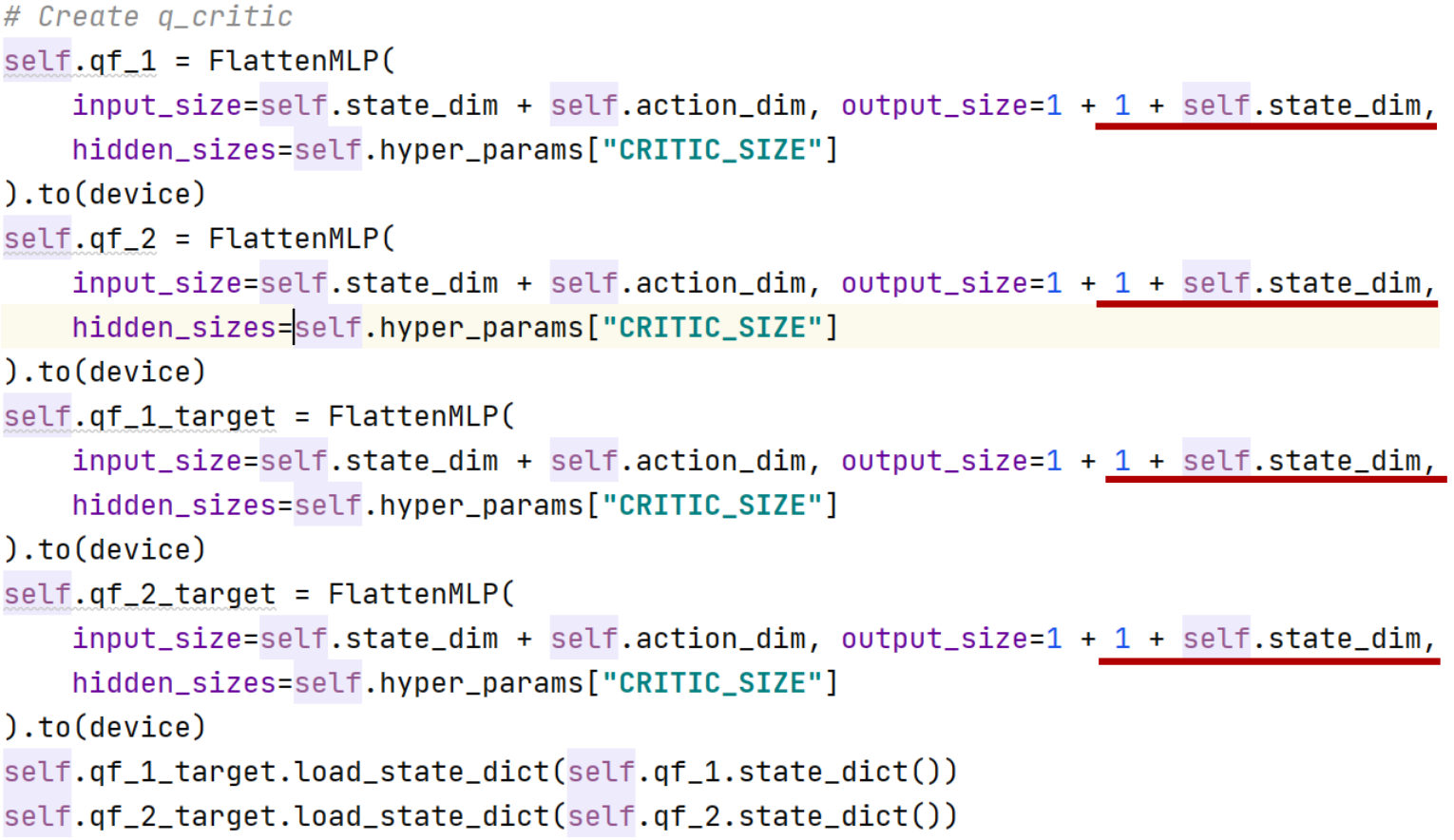
|
In the update step of SAC, we can compute model errors as follows:
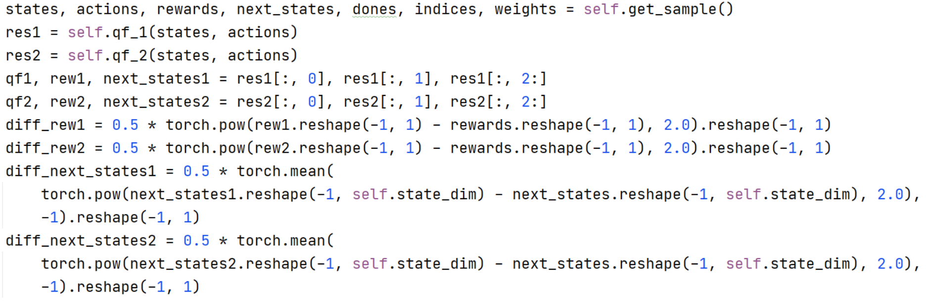
|
Then we can formulate MQN’s loss by summing model- and TD-errors as in Figure E.3. The coefficient of each loss adaptively changes by a dynamic method in (Liang & Zhang, 2020). Furthermore, we use the quantity to impose priorities to corresponding samples as in Figure E.4. These modifications are all for applying model-augmented -learning (MQL). Note that there is no hyper-parameters change. In a similar manner, we can apply MQL to other algorithms, e.g., TD3 (Fujimoto et al., 2018), and Rainbow (Hessel et al., 2018; van Hasselt et al., 2019). In the case of Rainbow, we use the context obtained by convolutional layers.
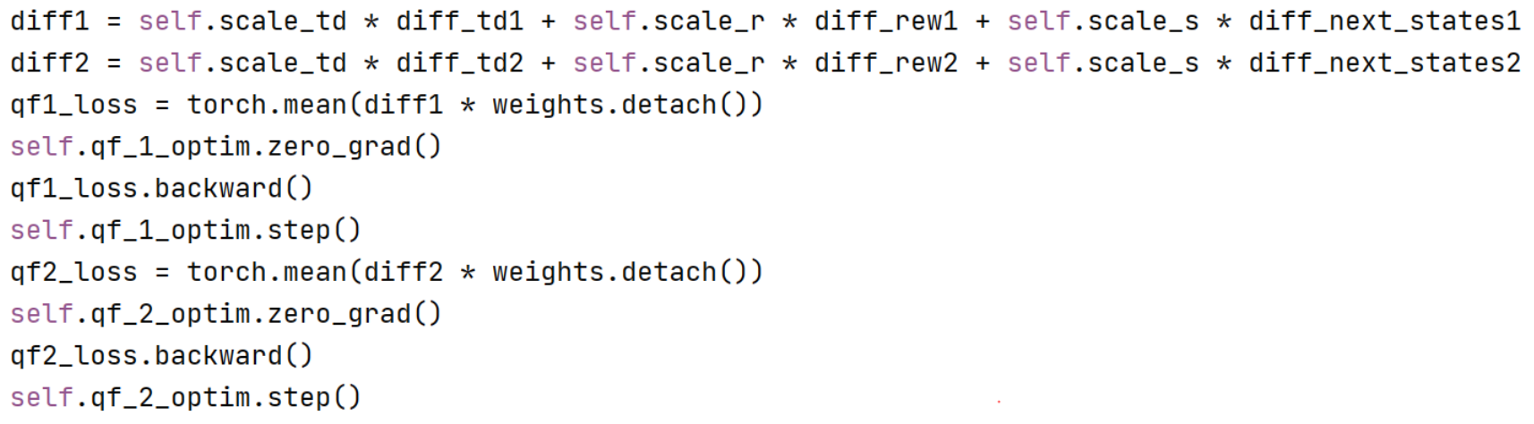
|
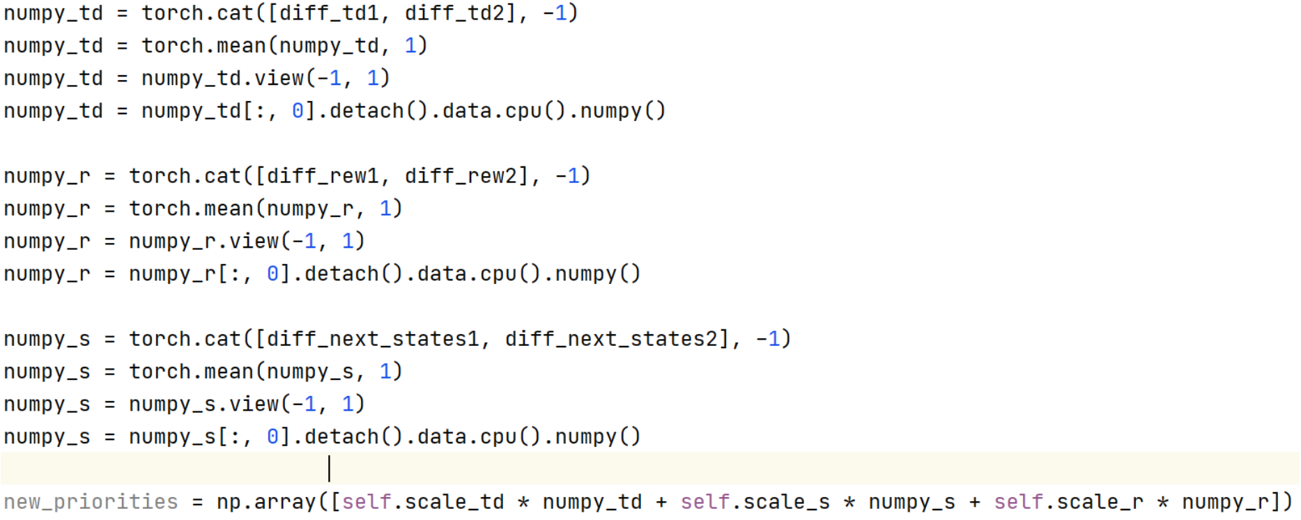
|
Appendix F Additional Experimental Results
We add efficient-Rainbow (van Hasselt et al., 2019)’s results on other Atari games. MRainbow-MPER also outperforms baselines in all tested cases.
| (a) Alien | (b) Asterix | (c) Gopher | (d) Kangaroo |
| Hopper-v3 |
Moreover, as we mentioned in Section D, to show that prior knowledge is crucial to MBRL, we provide an experimental result about one of the state-of-the-art MBRL methods, i.e., MBPO (Janner et al., 2019) with and without learning a termination function. To verify it, we increased the output dimension of an ensemble of dynamic models by one. Then we used the sigmoid function to learn the probability of the termination function with the binary cross-entropy loss. One can observe that the learning termination function is significantly harmful to the sample efficiency compared to the original MBPO in Figure F.2. The degraded result comes from wrongly computed TD-errors since computing the TD target depends heavily on the termination function.