An Efficient Model Order Reduction Scheme for Dynamic Contact in Linear Elasticity

We consider large-scale systems of differential-algebraic equations with unilateral constraints in the form

	$\displaystyle{\boldsymbol{M}}\ddot{{\boldsymbol{q}}}(t)+{\boldsymbol{K}}{\boldsymbol{q}}(t)={\boldsymbol{f}}(t)+{\boldsymbol{C}}^{T}{\boldsymbol{\lambda}},$		(1)
	$\displaystyle{\boldsymbol{C}}{\boldsymbol{q}}(t)+{\boldsymbol{b}}\geq 0,\quad{\boldsymbol{\lambda}}\geq 0,\quad{\boldsymbol{\lambda}}*({\boldsymbol{C}}{\boldsymbol{u}}(t)+{\boldsymbol{b}})=0$		(2)

where ${\boldsymbol{q}}(t)\in\mathbb{R}^{N}$ denotes the vector of nodal displacement variables, ${\boldsymbol{M}}\in\mathbb{R}^{N\times N}$ the symmetric positive definite mass matrix, ${\boldsymbol{K}}\in\mathbb{R}^{N\times N}$ the symmetric positive semi-definite stiffnes matrix, and ${\boldsymbol{f}}(t)\in\mathbb{R}^{N}$ the load vector. Furthermore, ${\boldsymbol{C}}\in\mathbb{R}^{m\times N}$ stands for the constraint matrix and ${\boldsymbol{b}}\in\mathbb{R}^{m}$ for a given initial clearance vector. The inequality signs in (2) are to be interpreted component-wise and stand for the discretized non-penetration conditions of all variables in the contact interface. Correspondingly, the vector of Lagrange multipliers ${\boldsymbol{\lambda}}\in\mathbb{R}^{m}$ enforces the constraint in the dynamic equation (1). The multiplier ${\boldsymbol{\lambda}}$, standing for the discretized contact pressure, is always positive and its inner product with the constraints satifies a complementarity condition.

In this paper, we will introduce a model order reduction method for the semi-discretized equations (1) that projects the nodal variables ${\boldsymbol{q}}$ onto a much smaller space while explicitly preserving the constraints and the Lagrange multipliers. For this purpose, the structure of the equations and the properties of the matrices as stated above are an appropriate starting point. Frictionless, adhesive-free normal contact in combination with small deformation theory and a linear-elastic material will lead to (1) if

• (i)

  the Lagrange multiplier method is used to enforce the non-penetration condition and

• (ii)

  the finite element method on matching meshes, i.e., node-to-node contact, is applied for the discretization in space.

Approaches like the augmented Lagrange method or the Nitsche method [25] lead to modifications that will not be considered here. The same holds for additional friction effects and node-to-segment contact.

For a contact problem with $k$ bodies that fits into the framework described so far, the mass matrix ${\boldsymbol{M}}$ will consist of $k$ blocks on the diagonal that stem from the discretizations of the individual bodies, and the same block-diagonal structure applies to the stiffness matrix ${\boldsymbol{K}}$. The constraint matrix ${\boldsymbol{C}}$ will then typically exhibit a sparse structure where each row stands for a node-to-node contact condition. We do not dive further into the details of various contact models and discretization schemes and refer instead to the standard references [17, 25]. But for the sake of a self-contained presentation, we shortly sketch the setting of the classical obstacle problem in the dynamic case.

Assuming as before frictionless, adhesive-free normal contact and a linear-elastic material as well as linear kinematics, we can express the dynamic contact problem in terms of the displacement field ${\boldsymbol{u}}({\boldsymbol{x}},t)\in\mathbb{R}^{d}$ and the contact pressure $p({\boldsymbol{x}},t)\in\mathbb{R}$ where $x\in\Omega\subset\mathbb{R}^{d},d=2$ or $d=3$, is the spatial variable and $t\in[t_{0},T]$ stands for the temporal variable. The boundary of the elastic body is decomposed into $\partial\Omega=\Gamma_{D}\cup\Gamma_{N}\cup\Gamma_{C}$ where the latter represents the contact interface. Using the outward normal vector ${\boldsymbol{n}}({\boldsymbol{x}})$ on the contact interface, the distance between the body and a given surface is described by the scalar gap function

$$g({\boldsymbol{x}},{\boldsymbol{u}})=\big({\boldsymbol{\xi}}({\boldsymbol{x}})-({\boldsymbol{x}}+{\boldsymbol{u}}({\boldsymbol{x}},t)\big)^{T}{\boldsymbol{n}}({\boldsymbol{x}}),\quad{\boldsymbol{x}}\in\Gamma_{C}.$$

(3)

Here, the point ${\boldsymbol{\xi}}({\boldsymbol{x}})$ on the obstacle’s surface is obtained by projection of ${\boldsymbol{x}}$ in outward normal direction. The contact problem in strong form is then given by the dynamic equations

$$\rho{\boldsymbol{u}}_{tt}-\mbox{div}{\boldsymbol{\sigma}}({\boldsymbol{u}})={\boldsymbol{F}}\quad\mbox{in }\Omega\times[t_{0},T]$$

(4)

subject to standard boundary conditions

$${\boldsymbol{\sigma}}({\boldsymbol{u}})\cdot{\boldsymbol{n}}={\boldsymbol{\tau}}\quad\mbox{on }\Gamma_{N}\times[t_{0},T],\qquad{\boldsymbol{u}}=0\quad\mbox{on }\Gamma_{D}\times[t_{0},T]$$

(5)

and furthermore subject to the contact conditions

$$g\geq 0,\quad p\geq 0,\quad g\cdot p=0\quad\mbox{on }\Gamma_{C}\times[t_{0},T].$$

(6)

As initial data,

$${\boldsymbol{u}}(\cdot,t_{0})={\boldsymbol{u}}_{0}\quad\mbox{and }\,{\boldsymbol{u}}_{t}(\cdot,t_{0})={\boldsymbol{v}}_{0}$$

(7)

are prescribed with given functions ${\boldsymbol{u}}_{0}$ and ${\boldsymbol{v}}_{0}$, respectively.

In (4) and (5), the constant $\rho$ denotes the mass density, ${\boldsymbol{F}}({\boldsymbol{x}},t)\in\mathbb{R}^{d}$ the volume force, ${\boldsymbol{\tau}}({\boldsymbol{x}},t)\in\mathbb{R}^{d}$ the surface traction, and ${\boldsymbol{\sigma}}({\boldsymbol{u}})\in R^{d\times d}$ the stress tensor given by

$${\boldsymbol{\sigma}}({\boldsymbol{u}})=\frac{E}{1+\nu}{\boldsymbol{e}}({\boldsymbol{u}})+\frac{\nu E}{(1+\nu)(1-2\nu)}\mbox{trace}({\boldsymbol{e}}({\boldsymbol{u}})){\boldsymbol{I}}$$

(8)

with Young’s modulus $E\geq 0$, Poisson’s ratio $-1\leq\nu\leq 0.5$ and linearized strain tensor

$${\boldsymbol{e}}({\boldsymbol{u}})=\frac{1}{2}(\nabla{\boldsymbol{u}}+\nabla{\boldsymbol{u}}^{T})\in\mathbb{R}^{d\times d}.$$

(9)

In order to pass to a weak formulation of the obstacle problem, we introduce the function spaces

	$\displaystyle\mathcal{V}$	$\displaystyle:=$	$\displaystyle\left\{{\boldsymbol{v}}\in H^{1}(\Omega)^{d}:{\boldsymbol{v}}=0\,\mbox{on }\Gamma_{D}\right\},$		(10)
	$\displaystyle\mathcal{L}$	$\displaystyle:=$	$\displaystyle\left\{\mu\in H^{1/2}(\Gamma_{C})^{\prime}:\int_{\Gamma_{C}}\mu w\,ds\geq 0\,\,\forall w\in H^{1/2}(\Gamma_{C}),w\geq 0\right\}$		(11)

and the abstract notation

$$\langle\rho{\boldsymbol{u}}_{tt},{\boldsymbol{v}}\rangle:=\int_{\Omega}{\boldsymbol{v}}^{T}\rho{\boldsymbol{u}}_{tt}dx,\,\,a({\boldsymbol{u}},{\boldsymbol{v}}):=\int_{\Omega}{\boldsymbol{\sigma}}({\boldsymbol{u}}):{\boldsymbol{e}}({\boldsymbol{v}})dx,\,\,\langle\ell,{\boldsymbol{v}}\rangle:=\int_{\Omega}{\boldsymbol{v}}^{T}{\boldsymbol{F}}dx+\int_{\Gamma_{N}}{\boldsymbol{v}}^{T}{\boldsymbol{\tau}}ds.$$

(12)

The non-penetration condition in weak form with test function $\mu\in{\cal L}$ is recast as

$$0\leq\int_{\Gamma_{C}}g\mu ds=\int_{\Gamma_{C}}g(\mu-p)ds=-\int_{\Gamma_{C}}{\boldsymbol{u}}^{T}{\boldsymbol{n}}(\mu-p)ds+\int_{\Gamma_{C}}({\boldsymbol{\xi}}-{\boldsymbol{x}})^{T}{\boldsymbol{n}}(\mu-p)ds.$$

(13)

The last two integrals give rise to the definitions of the bilinear form

$$b_{c}({\boldsymbol{v}},p):=-\int_{\Gamma_{C}}{\boldsymbol{v}}^{T}{\boldsymbol{n}}\cdot p\,ds$$

(14)

on ${\cal V}\times{\cal L}$ and the linear form on $\cal L$

$$\langle{m},p\rangle:=\int_{\Gamma_{C}}({\boldsymbol{\xi}}-{\boldsymbol{x}})^{T}{\boldsymbol{n}}p\,ds.$$

(15)

Using these definitions, the weak form of the dynamic contact problem is stated as follows: For each $t\in[t_{0},T]$ find the displacement field ${\boldsymbol{u}}(\cdot,t)\in\mathcal{V}$ and the contact pressure $p(\cdot,t)\in\mathcal{L}$ such that

	$\displaystyle\langle\rho{\boldsymbol{u}}_{tt},{\boldsymbol{v}}\rangle+a({\boldsymbol{u}},{\boldsymbol{v}})$	$\displaystyle=\langle\ell,{\boldsymbol{v}}\rangle+b_{c}({\boldsymbol{v}},p)\quad$		$\displaystyle\mbox{for all }{\boldsymbol{v}}\in\mathcal{V},$		(16)
	$\displaystyle b_{c}({\boldsymbol{u}},\mu-p)+\langle{m},\mu-p\rangle$	$\displaystyle\geq 0\quad$		$\displaystyle\mbox{for all }\mu\in\mathcal{L}.$

The system (16) is discretized with respect to the spatial varibale by applying the standard Galerkin projection ${\boldsymbol{u}}({\boldsymbol{x}},t)\doteq\sum_{i=1}^{N}{\boldsymbol{\phi}}_{i}({\boldsymbol{x}})q_{i}(t)={\boldsymbol{\Phi}}({\boldsymbol{x}}){\boldsymbol{q}}(t)$ with basis functions ${\boldsymbol{\phi}}_{i}$ and nodal variables ${\boldsymbol{q}}=(q_{1},\ldots,q_{N})$ to the displacement field. If the contact condition is simply expressed in terms of the distance between a node ${\boldsymbol{x}}_{j}\in\Gamma_{C},i=1,\ldots,m$, and the obstacle, the integral over $\Gamma_{C}$ in the weak dynamic equation is replaced by a sum

$$\int_{\Gamma_{C}}{\boldsymbol{v}}^{T}{\boldsymbol{n}}\cdot p\,ds\doteq\sum_{j=1}^{m}A_{j}{\boldsymbol{v}}({\boldsymbol{x}}_{j})^{T}{\boldsymbol{n}}({\boldsymbol{x}}_{j})\cdot p({\boldsymbol{x}}_{j},t),\quad A_{j}:\mbox{area around node }{\boldsymbol{x}}_{j}.$$

(17)

In the same way, the unilateral constraint is discretized. Putting finally ${\boldsymbol{\lambda}}(t):=(p({\boldsymbol{x}}_{1},t),\ldots,p({\boldsymbol{x}}_{m},t))$ as discrete pressure variable, the semi-discretized equations (1) and (2) follow in the usual way, with the matrix ${\boldsymbol{C}}\in\mathbb{R}^{m\times N}$ being an indicator matrix for the nodes in the contact interface and ${\boldsymbol{b}}\in\mathbb{R}^{m}$ the offset of the contact. Note that only a few displacements are involved for the contact condition and hence most of the entries of the matrix ${\boldsymbol{C}}$ are zero.

In the stationary case, we can recast the generic semi-discretized formulation (1) and (2) as minimization problem

$$\min_{{\boldsymbol{q}}\in\mathbb{R}^{N},{\boldsymbol{\lambda}}\in\mathbb{R}_{+}^{m}}\frac{1}{2}{\boldsymbol{q}}^{T}{\boldsymbol{K}}{\boldsymbol{q}}-{\boldsymbol{q}}^{T}{\boldsymbol{f}}-{\boldsymbol{\lambda}}^{T}({\boldsymbol{C}}{\boldsymbol{q}}+{\boldsymbol{b}}).$$

(18)

Note that the requirement ${\boldsymbol{\lambda}}\in\mathbb{R}_{+}^{m}$ enforces the positivity of the contact pressure and, simultaneously, the non-penetration condition. The corresponding KKT-conditions read

$$\begin{array}[]{l}{\boldsymbol{K}}{\boldsymbol{q}}-{\boldsymbol{f}}-{\boldsymbol{C}}^{T}{\boldsymbol{\lambda}}=0,\\ {\boldsymbol{C}}{\boldsymbol{q}}+{\boldsymbol{b}}\geq 0,\quad{\boldsymbol{\lambda}}\geq 0,\quad{\boldsymbol{\lambda}}*({\boldsymbol{C}}{\boldsymbol{q}}+{\boldsymbol{b}})=0.\end{array}$$

(19)

Next, assuming a positive-definite stiffness matrix, we eliminate the displacements ${\boldsymbol{q}}$ from the KKT-conditions (19) via

$${\boldsymbol{q}}={\boldsymbol{K}}^{-1}({\boldsymbol{f}}+{\boldsymbol{C}}^{T}{\boldsymbol{\lambda}})$$

(20)

and insert this expression into the constraint equations. This results in

$$\begin{array}[]{rcc}{\boldsymbol{C}}{\boldsymbol{K}}^{-1}{\boldsymbol{f}}+{\boldsymbol{C}}{\boldsymbol{K}}^{-1}{\boldsymbol{C}}^{T}{\boldsymbol{\lambda}}+{\boldsymbol{b}}&\geq&0,\\ {\boldsymbol{\lambda}}&\geq&0,\\ {\boldsymbol{\lambda}}*({\boldsymbol{C}}{\boldsymbol{K}}^{-1}{\boldsymbol{f}}+{\boldsymbol{C}}{\boldsymbol{K}}^{-1}{\boldsymbol{C}}^{T}{\boldsymbol{\lambda}}+{\boldsymbol{b}})&=&0.\end{array}$$

(21)

Using the abbreviations

$${\boldsymbol{A}}:={\boldsymbol{C}}{\boldsymbol{K}}^{-1}{\boldsymbol{C}}^{T}\in\mathbb{R}^{m\times m},\quad{\boldsymbol{B}}:={\boldsymbol{C}}{\boldsymbol{K}}^{-1}{\boldsymbol{f}}+{\boldsymbol{b}}\in\mathbb{R}^{m},$$

(22)

the equations (21) read

$$\begin{array}[]{rcc}{\boldsymbol{B}}+{\boldsymbol{A}}{\boldsymbol{\lambda}}&\geq&0,\\ {\boldsymbol{\lambda}}&\geq&0,\\ {\boldsymbol{\lambda}}*({\boldsymbol{B}}+{\boldsymbol{A}}{\boldsymbol{\lambda}})&=&0.\end{array}$$

(23)

The LCP problem (23) may be solved by standard methods from constrained optimization, see below for more details. Note that tasks like the detection of active contact nodes are thus transferred to the LCP solver.

In the transient case, the dynamic equations (1) must be discretized in time. As straightforward and unconditionally stable method, we apply the implicit Euler scheme, i.e., the first order backward differentiation formula. For this purpose, the second order derivative is replaced by the finite difference

$$\ddot{{\boldsymbol{q}}}(t+h)\approx\frac{1}{h^{2}}\big({\boldsymbol{q}}(t+h)-2{\boldsymbol{q}}(t)+{\boldsymbol{q}}(t-h)\big)$$

(24)

with time stepsize $h$. Note that the finite difference $\dot{{\boldsymbol{q}}}(t+h)\approx({\boldsymbol{q}}(t+h)-{\boldsymbol{q}}(t))/h$ for the velocity is hidden in (24), and due to the second order time derivative, the implicit Euler leads here to a two-step method. Since (24) possesses first order of accuracy only, one can apply other integration schemes instead, e.g. the generalized-$\alpha$ method, which is very common in structural mechanics, cf. [24].

In this paper, however, we continue working with the implicit Euler method as our main interest focuses on the model order reduction scheme. Moreover, dynamic contact involves frequent discontinuities that might impair the convergence of a higher order time integration method. Inserting (24) into (1) leads to

$${\boldsymbol{M}}\left({\boldsymbol{q}}(t+h)-2{\boldsymbol{q}}(t)+{\boldsymbol{q}}(t-h)\right)+h^{2}{\boldsymbol{K}}{\boldsymbol{q}}(t+h)=h^{2}{\boldsymbol{f}}(t+h)+h^{2}{\boldsymbol{C}}^{T}{\boldsymbol{\lambda}}(t+h)$$

(25)

Assuming that the previous time steps are known, (25) may be resolved for ${\boldsymbol{q}}(t+h)$,

$${\boldsymbol{q}}(t+h)=({\boldsymbol{M}}+h^{2}{\boldsymbol{K}})^{-1}(h^{2}{\boldsymbol{f}}(t+h)+h^{2}{\boldsymbol{C}}^{T}{\boldsymbol{\lambda}}(t+h)+2{\boldsymbol{M}}{\boldsymbol{q}}(t)-{\boldsymbol{M}}{\boldsymbol{q}}(t-h)).$$

(26)

Now the same procedure as in the static case may be applied. Inserting (26) into the constraints (2) again leads to an LCP. With the definitions

	$\displaystyle{\boldsymbol{A}}$	$\displaystyle:=$	$\displaystyle h^{2}{\boldsymbol{C}}({\boldsymbol{M}}+h^{2}{\boldsymbol{K}})^{-1}{\boldsymbol{C}}^{T},$		(27)
	$\displaystyle{\boldsymbol{B}}$	$\displaystyle:=$	$\displaystyle{\boldsymbol{C}}({\boldsymbol{M}}+h^{2}{\boldsymbol{K}})^{-1}(h^{2}{\boldsymbol{f}}(t+h)+2{\boldsymbol{M}}{\boldsymbol{u}}(t)-{\boldsymbol{M}}{\boldsymbol{u}}(t-h))+{\boldsymbol{b}}$		(28)

we again arrive at the LCP (23), which here has to be solved in each time step.

We remark that the two-step time discretization requires initial values ${\boldsymbol{q}}(t_{0})$ and ${\boldsymbol{q}}(t_{0}+h)$ to start. E.g., if ${\boldsymbol{q}}_{0}$ and $\dot{{\boldsymbol{q}}}_{0}$ as initial displacement and velocity are given, one can compute ${\boldsymbol{q}}(t_{0}+h)={\boldsymbol{q}}_{0}+h\dot{{\boldsymbol{q}}}_{0}$ by an explicit Euler step and then continue with the two-step formula (25). The Lagrange multiplier ${\boldsymbol{\lambda}}$, on the other hand, does not require an initial value, and it is computed in each time step as an implicitly given function of ${\boldsymbol{q}}$. In the terminology of differential-algebraic equations, this means that ${\boldsymbol{q}}$ stands for the differential variables while the algebraic variables ${\boldsymbol{\lambda}}$ possess no memory. If the unilateral constraints were replaced by equality constraints ${\boldsymbol{C}}{\boldsymbol{q}}+{\boldsymbol{b}}=0$, the index of the resulting differential-algebraic equation would equal 3, which means that special care must be taken for the time integration [6, 16, 24].

Another remark concerns the treatment of impact situations. In the presented time discretization, impacts are not specifically identified by means of computing an impact velocity and a corresponding coefficient of restitution. Instead, the LCP solution in each time step implicitly enforces a plastic impact solution that might lead to a loss in kinetic energy.

The core of our proposed solution algorithm consists of the efficient solution of the LCP problem (23). One way for solving LCPs is the usage of so-called NCP-functions $\phi^{\text{NCP}}$. An NCP-function $\phi^{\text{NCP}}:\mathbb{R}^{2}\to\mathbb{R}$ is characterized by the property

$$\phi^{\text{NCP}}(a,b)=0\quad\Leftrightarrow\quad a\geq 0,\ b\geq 0,\ ab=0.$$

(29)

Two examples of NCP-functions are:

	$\displaystyle\phi_{1}^{\text{NCP}}(a,b)$	$\displaystyle=$	$\displaystyle\min(a,b),$		(30)
	$\displaystyle\phi_{2}^{\text{NCP}}(a,b)$	$\displaystyle=$	$\displaystyle\sqrt{a^{2}+b^{2}}-a-b.$		(31)

The first function (30) is not suitable for computational purposes because of its non-smoothness. The second NCP-function is also known as the Fischer-Burmeister-function [12]. Thus for solving an LCP the following two formulations (32) and (33) are equivalent:

$$\begin{array}[]{rcc}{\boldsymbol{B}}+{\boldsymbol{A}}{\boldsymbol{\lambda}}&\geq&0,\\ {\boldsymbol{\lambda}}&\geq&0,\\ {\boldsymbol{\lambda}}*({\boldsymbol{B}}+{\boldsymbol{A}}{\boldsymbol{\lambda}})&=&0.\end{array}$$

(32)

$\Longleftrightarrow$

$$\phi_{2}^{\text{NCP}}\left({\boldsymbol{B}}+{\boldsymbol{A}}{\boldsymbol{\lambda}},{\boldsymbol{\lambda}}\right)=0.$$

(33)

Equation (33) may be solved by Newton’s method, but here we apply a much more efficient method in terms of Lemke’s algorithm (see [8], Sect. 4.4.5). Specifically, we use the Python implementation of the algorithm [18].

One way to obtain the reduction matrix ${\boldsymbol{Q}}$ is to use modal reduction. Setting up the eigenvalue problem in the unconstrained case

$$\omega^{2}{\boldsymbol{M}}{\boldsymbol{y}}={\boldsymbol{K}}{\boldsymbol{y}}$$

(35)

and taking the first $n_{r}$ eigenvectors, the matrix ${\boldsymbol{Q}}$ is then defined by

$${\boldsymbol{Q}}=\left\{{\boldsymbol{y}}_{1},\cdots,{\boldsymbol{y}}_{n_{r}}\right\}.$$

(36)

A more recent technique are the Krylov subspace methods [2, 22]. The reduction is defined by

$${\boldsymbol{Q}}=\left\{{\boldsymbol{K}}_{\omega}^{-1}{\boldsymbol{f}},{\boldsymbol{K}}_{\omega}^{-1}{\boldsymbol{M}}{\boldsymbol{K}}_{\omega}^{-1}{\boldsymbol{f}},\cdots,({\boldsymbol{K}}_{\omega}^{-1}{\boldsymbol{M}})^{n_{r}-1}{\boldsymbol{K}}_{\omega}^{-1}{\boldsymbol{f}}\right\}$$

(37)

The Krylov vectors can be computed by the Arnoldi algorithm, which delivers an orthonormal basis of the subspace. Inserting the reduction (34), where ${\boldsymbol{Q}}$ is defined by (36) or (37), into the differential equation (1) and multiplying by ${\boldsymbol{Q}}^{T}$ from the left, we obtain the reduced equation

$$\hat{{\boldsymbol{M}}}\ddot{{\boldsymbol{v}}}+\hat{{\boldsymbol{K}}}{\boldsymbol{v}}={\boldsymbol{Q}}^{T}\left({\boldsymbol{f}}(t)+{\boldsymbol{C}}^{T}{\boldsymbol{\lambda}}(t)\right)$$

(38)

where $\hat{{\boldsymbol{M}}}={\boldsymbol{Q}}^{T}{\boldsymbol{M}}{\boldsymbol{Q}}$, $\hat{{\boldsymbol{K}}}={\boldsymbol{Q}}^{T}{\boldsymbol{K}}{\boldsymbol{Q}}$ $\in\mathbb{R}^{n_{r}\times n_{r}}$ are the reduced matrices.

Using (38), moreover the reduced time discretization follows easily as

$${\boldsymbol{v}}(t+h)=\left(\hat{{\boldsymbol{M}}}+h^{2}\hat{{\boldsymbol{K}}}\right)^{-1}\left(h^{2}{\boldsymbol{Q}}^{T}{\boldsymbol{f}}(t+h)+h^{2}{\boldsymbol{Q}}^{T}{\boldsymbol{C}}^{T}{\boldsymbol{\lambda}}(t+h)+2\hat{{\boldsymbol{M}}}{\boldsymbol{v}}(t)-\hat{{\boldsymbol{M}}}{\boldsymbol{v}}(t-h))\right)$$

(39)

We stress that (39) contains only operations with complexity $O(n_{r})$ or $O(m)$. Though ${\boldsymbol{Q}}\in\mathbb{R}^{N\times n_{r}}$, the acting force ${\boldsymbol{f}}(t+h)$ has only a few entries and the Lagrange multiplier ${\boldsymbol{\lambda}}$ is still of dimension $m$.

Next, we introduce a modification of our approach which is inspired by the fact that often the dominant influence on the dynamics of the system stems from the nodes located on the contact interface. In other words, we distinguish between the nodal variables on the contact interface, so-called master nodes and the ones outside of the contact interface, the so-called slave nodes. We adopt this technique from structural dynamics, see Craig and Bampton [21].

Let ${\boldsymbol{q}}=({\boldsymbol{q}}_{M},{\boldsymbol{q}}_{S})^{T}\in\mathbb{R}^{N}$ the permuted solution vector such that we distinguish between master and slave nodes. Then the corresponding permuted matrices and the permuted force vector are given by

$\displaystyle{\boldsymbol{M}}=\begin{pmatrix}{\boldsymbol{M}}_{MM}&{\boldsymbol{M}}_{MS}\\ {\boldsymbol{M}}_{SM}&{\boldsymbol{M}}_{SS}\end{pmatrix},\quad{\boldsymbol{K}}=\begin{pmatrix}{\boldsymbol{K}}_{MM}&{\boldsymbol{K}}_{MS}\\ {\boldsymbol{K}}_{SM}&{\boldsymbol{K}}_{SS}\end{pmatrix},\quad{\boldsymbol{F}}=\begin{pmatrix}{\boldsymbol{F}}_{M}\\ {\boldsymbol{F}}_{S}\end{pmatrix}.$

(40)

Due to the fact that the constraint matrix affects only the dynamics of the slave nodes it holds

$\displaystyle{\boldsymbol{C}}=\begin{pmatrix}{\boldsymbol{C}}_{M}\\ {\boldsymbol{C}}_{S}\end{pmatrix},\quad{\boldsymbol{C}}_{S}=0.$

(41)

The constraint matrix refers only to the master nodes. A crucial assumption is now that the influence acceleration term for the slave nodes in the dynamic equation can be neglected, and the same for the force term. This yields a coupling equation between the master and slave node via

$${\boldsymbol{K}}_{SM}{\boldsymbol{q}}_{M}+{\boldsymbol{K}}_{SS}{\boldsymbol{q}}_{S}=0$$

(42)

Since we want to preserve the contact nodes and only reduce the slave nodes, we keep the structure of the master nodes fixed, i.e, ${\boldsymbol{u}}_{M}=0.$ Then due to (41) the dynamical system is given by

$${\boldsymbol{M}}_{SS}\ddot{{\boldsymbol{q}}}_{S}+{\boldsymbol{K}}_{SS}{\boldsymbol{q}}_{S}={\boldsymbol{F}}_{S}$$

(43)

Instead for the full system, we compute the transformation matrix for the slave system (43) using the Arnoldi method, which yields

$${\boldsymbol{Q}}_{S}:=\left\{{\boldsymbol{K}}_{SS}^{-1}{\boldsymbol{F}}_{S},{\boldsymbol{K}}_{SS}^{-1}{\boldsymbol{M}}_{SS}{\boldsymbol{K}}_{SS}^{-1}{\boldsymbol{F}}_{S},\cdots,({\boldsymbol{K}}_{SS}^{-1}{\boldsymbol{M}}_{SS})^{n-1}{\boldsymbol{K}}_{SS}^{-1}{\boldsymbol{F}}_{S}\right\}.$$

(44)

Using (42), we obtain the complete transformation matrix that includes the relation between the master and slave nodes,

$\displaystyle{\boldsymbol{Q}}_{CB}=\begin{pmatrix}{\boldsymbol{I}}_{M}&0\\ -{\boldsymbol{K}}_{SS}^{-1}{\boldsymbol{K}}_{SM}&{\boldsymbol{Q}}_{S}\end{pmatrix}$

(45)

The transformation matrix ${\boldsymbol{Q}}_{CB}$ with the partitioning of master and slave nodes in the fashion of the Craig-Bampton method provides an alternative for reducing the transient contact problem (39). Regardless whether we employ ${\boldsymbol{Q}}$ from the reduction (37) or ${\boldsymbol{Q}}_{CB}$, the computation of the transformation can be done in an a priori offline phase and does not require solution trajectories, i.e., snapshots, of the full system.

We consider the unit square $\Omega=[0,1]\times[0,1]$ under the assumption of plane stress. The parameters in dimensionless form are $\rho=1,E=1000,\nu=0.3$. The left edge is fixed by means of zero Dirichlet boundary conditions. We discretize the example by 1600 quadrilateral elements, which lead to $N=3386$ DOF. An interior contact interface is predefined by a fixed number of $m$ discretization points where each such point is represented by double nodes. This kind of data structure allows us to distinguish the nodes placed on the contact interface from the remaining nodes. Note that the node-to-node non-penetration condition acts only in $x$-direction while the DOF in $y$-direction may move freely.

An oscillating force acts on the right side of the domain which affects the contact interface by opening and closing the tear over time. The problem setup and the mesh are illustrated in Figure 1. Two sensors are placed for the data extraction in order to compare the displacements of the full and the reduced model. Before starting the reduction method we eliminate the fixed degrees of freedom due to the Dirichlet boundary condition. Overall, there are $4m$ displacement variables associated with the contact nodes due to the relation $n_{c}=4m$

We continue with a comparison of the reduction results with and without Craig-Bampton splitting, which was discussed in Subsection 4.2. To guarantee a fair comparison of the two methods, we choose the same number of basis functions in both cases. In case of using no splitting, the basis consists of only Krylov vectors, whereas in the splitting case, the basis consists of a few Krylov vectors ($n_{k}$) and additionally the contact nodes ($n_{c}$ ), i.e., $n_{r}=n_{k}+n_{c}.$ The Figure 8 shows the comparison of both reduction approaches with the full model, referring to the scenario of Fig. 1. We can observe an increase of accuracy in case of using the splitting of Craig-Bampton. This holds also for the second sensor node and the displacements in $y$-direction.

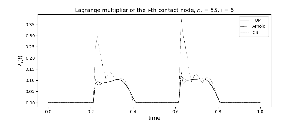
Furthermore, the Lagrange multipliers ${\boldsymbol{\lambda}}(t)$ exhibit an interesting behavior. We observe that ROM without splitting produces contact pressures that are quite different from those of the FOM, while the Craig-Bampton splitting yields values that agree well with the FOM. Both approaches guarantee positivity of the Lagrange multiplicator whenever the contact is activated. An explanation of this deviation with respect to the Lagrange multipliers in case of no splitting is as follows. The projection matrix ${\boldsymbol{Q}}$ in (34) alters the nodewise distribution of the pressure on the contact variables considerably and involves spatial basis functions with large support. Splitting of variables, on the other hand, by means of ${\boldsymbol{Q}}_{CB}$ in (45) preserves the contact variables and thus the Lagrange multipliers. In Figure 8 the $x$-displacement in the sensor node 1 for both reduction approaches and the FOM is displayed, along with the corresponding Lagrange multiplier. The switching between contact, where the multiplier is positive, and positive gap with vanishing multiplier can be nicely observed.

References

- [1] Siemens AG. Nastran. https://www.plm.automation.siemens.com/de_de/products/simcenter/nastran/.
- [2] Z. Bai. Krylov subspace techniques for reduced-order modeling of large-scale dynam-ical systems. Applied Numerical Mathematics, 43:9–44, 2002.
- [3] M. Balajewiec, D. Amsallem, and C. Farhat. Projection-based model reduction for contact problems. Int. J. Numer. Meth. Engng, 106:pp. 644–663, 2015.
- [4] U. Baur, P. Benner, and L. Feng. Model order reduction for linear and nonlinear systems: a system-theoretic perspective. Max Planck Institute Magdeburg Preprints, MPIMD/14-07, 2014.
- [5] U. Baur, P. Benner, and L. Feng. Model order reduction for linear and nonlinear systems: a system-theoretic perspective. Archives of Computational Methods in Engineering, 2014.
- [6] K. E. Brenan, S. L. Campbell, and L. R. Petzold. The Numerical Solution of Initial Value Problems in Ordinary Differential-Algebraic Equations. SIAM, Philadelphia, 1996.
- [7] S. Chaturantabut and D.C. Sorensen. Discrete empirical interpolation for nonlinear model reduction. 32:4316 – 4321, 01 2010.
- [8] R. W. Cottle, J. S. Pang, and Richard E. Stone. The Linear Complementarity Problem. SIAM, 2009.
- [9] R.W. Cottle, J.S. Pang, and R.E. Stone. The linear complementarity problem. San Diego, CA: Academic, 1992.
- [10] M. Eigner, T. Gilz, and R. Zafirov. Interdisziplinäre produktentwicklung - modellbasiertes systems engineering. PLM Portal, 2012.
- [11] C. Farhat, P. Avery, T. Chapman, and J. Cortial. Dimensional reduction of nonlinear finite element dynamic models with finite rotations and energy-based mesh sampling and weighting for computational efficiency. International Journal for Numerical Methods in Engineering, 98(9):625–662, 2014.
- [12] A. Fischer. A special newton-type optimization method. Optimization, 24:pp. 269–284, 1992.
- [13] A. Francavilla and O.C. Zienkiewicz. A note on numerical computation of elastic contact problems. International Journal for Numerical Methods in Engineering, 9:pp. 913–924, 1975.
- [14] P. Gill, W. Murry, and M. Wright. Practical Optimization. Academic Press, 4nd edition, 1981.
- [15] Ansys GmbH. Ansys. http://www.ansys.com/Solutions/Solutions-by-Application/Structures.
- [16] E. Hairer, Ch. Lubich, and M. Roche. The Numerical Solution of Differential-Algebraic Equations by Runge-Kutta Methods. Lecture Notes in Mathematics Vol. 1409. Springer, Heidelberg, 1989.
- [17] N. Kikuchi and J.T. Oden. Contact Problems in Elasticity. SIAM, 1988.
- [18] A. Lamperski. Python: lemkelcp 0.1. https://pypi.org/project/lemkelcp/.
- [19] C. X. Li and S. L. Wu. A note on the unique solution of linear complementarity problem. Cogent Mathematics, page DOI: 10.1080/23311835.2016.1271268, 2016.
- [20] M.J.D. Powell. A method for nonlinear constraints in minimization problems. Academic Press, in optimization ed. by r. fletcher edition, 1969.
- [21] D. J. Rixen. A dual craig–bampton method for dynamic substructuring. Journal of Computational and applied mathematics, 168(1-2):383–391, 2004.
- [22] B. Salimbahrami and B. Lohmann. Order reduction of large scale second-order systems using krylov subspace methods. Linear Algebra and its Applications, 415:385–405, 2005.
- [23] S. Salimbahrami and B. Lohmann. Order reduction of large scale second-order systems using krylov subspace methods. Linear Algebra and its Applications, 415:385–405, 2006.
- [24] B. Simeon. Computational flexible multibody dynamics. Springer, 2013.
- [25] P. Wriggers. Computational Contact Mechanics. Springer, 2006.