Algebraic branch points at all loop orders from positive kinematics and wall crossingPreprint: LCTP-21-04

Amplitudes in $\mathcal{N}=4$ pSYM are an ideal testing ground for exploring the analytic structure of planar scattering amplitudes. For instance, amplitudes in $\mathcal{N}=4$ pSYM have a finite number of branch points associated with solutions to the Landau equations and are expected to have a finite radius of convergence in perturbation theory Prlina:2018ukf. Significant progress has been made in understanding the structure of $\mathcal{N}=4$ pSYM amplitudes beyond Feynman diagrams. At weak coupling, deep geometric structures, such as the amplituhedron, have emerged that provide both powerful computational techniques for computing integrands at any loop order and a radically different perspective on the nature of locality and unitarity Arkani-Hamed:2013jha; Arkani-Hamed:2017vfh; Herrmann:2020qlt; ArkaniHamed:2012nw; Kojima:2020tjf. At strong coupling, holographic calculations provide non-trivial predictions for the behavior of $\mathcal{N}=4$ pSYM amplitudes in the form of the BDS-ansatz Anastasiou:2003kj; Bern:2005iz; Alday:2007hr and its generalizations Alday:2009dv; Yang:2010as. Other formalisms motivated by the duality between Wilson loops and scattering amplitudes have also emerged Brandhuber:2007yx; Alday:2010ku; CaronHuot:2010ek; Eden:2011yp; Basso:2013vsa; He:2020lcu; He:2020uxy; He:2021esx.

MHV amplitudes in $\mathcal{N}=4$ pSYM are particularly simple and have been useful litmus tests for conjectures. MHV $n$-point amplitudes are transcendental functions of fixed weight at each loop order that can be expressed in terms of multi-polylogarithms (MPLs) at all orders calculated to date Goncharov:2010jf; Gaiotto:2011dt; 2011arXiv1105.2076G; ArkaniHamed:2012nw; Golden:2013xva; Duhr:2014woa; GONCHAROV1995197.³³ 3 Using the Grassmannian form of $\mathcal{N}=4$ pSYM loop integrands, one can directly show all integrals in the MHV (and NMHV) sector can be written as iterated integrals of $d\log$-forms ArkaniHamed:2012nw. Unfortunately, this does not necessarily mean they integrate to a function that can be written in terms of MPLs Brown:2020rda. These transcendental functions of weight $W$, $F_{W}$, are the generalizations of logarithms that obey extremely nice properties. Primarily, the symbol provides a map from the amplitude to a sum of $W$-fold tensor products:

$$F\rightarrow\sum F^{\phi_{\alpha_{1}},\phi_{\alpha_{2}},\ldots,\phi_{\alpha_{W}}}_{0}[\log(\phi_{\alpha_{1}})\otimes\log(\phi_{\alpha_{2}})\otimes\ldots\otimes\log(\phi_{\alpha_{W}})]\ ,$$

(1)

where $F_{0}$ are rational numbers. Each factor in the tensor product behaves similarly to a logarithm, leading to properties like

$$[\ldots\otimes\log(\phi_{1}\phi_{2})\otimes\ldots]=[\ldots\otimes\log(\phi_{2})\otimes\ldots]+[\ldots\otimes\log(\phi_{1})\otimes\ldots]\ .$$

(2)

The $\phi_{i}$ in eq. (1) are functions of external kinematic data and correspond to branch points of $F_{W}$. The set of all $\phi$ that can appear in eq. (1) is called the symbol alphabet of $F_{W}$.

Scattering amplitudes are functions on kinematic space. The positive kinematic region is a region of kinematic space where planar gauge theory amplitudes are conjectured to have no poles or branch cuts. More precisely, in all examples studied to date, the Landau equations admit no solutions when the external data is taken to be in the positive kinematic region. The positive kinematic region for a given ordering of externals, $\alpha\in\textrm{Perm}[1,2,\ldots,n]$, is associated with the region where all planar variables are positive definite,

$$X_{i,j}=\left(\sum_{a=i}^{j-1}p_{\alpha(a)}\right)^{2}>0\ ,$$

(3)

along with additional constraints Golden:2013xva; Arkani-Hamed:2017vfh; Arkani-Hamed:2019rds. Although not well understood, the positive kinematic region implicitly appears in many computations. For example, the integrands that appear in open superstring scattering amplitudes are generically divergent unless evaluated in the positive kinematic region Arkani-Hamed:2019mrd; Sen:2019jpm. Therefore, when evaluating superstring integrands without using string field theory techniques or taking sophisticated Pochhammer contours in the string moduli space Witten:2013pra, one must implicitly work in the positive kinematic region, only taking an analytic continuation to generic momentum configurations at the end of the calculation. Again, we emphasize that the physical significance of the positive kinematic region remains mysterious and its importance has been found through direct computation.

Since we are studying the positive kinematic region of massless planar gauge theory amplitudes in 4 dimensions, we parameterize our external kinematic data using momentum twistors Golden:2013xva; $Z_{i}^{A}$ is the momentum twistor of state $i$ and the $A$ index transforms in the fundamental representation of the dual conformal algebra, $SU(2,2)$. Individual momentum twistors are projective:

$$Z_{i}^{A}\sim t_{i}Z_{i}^{A}\ .$$

(4)

Therefore, the kinematic space of the $n$-point amplitude can be interpreted as a quotient of the Grassmannian, $Gr(4,n)/T$, where $T$ acts on columns by a re-scaling. The positive kinematic region is then a quotient of the positive Grassmannian, $Gr_{+}(4,n)/T$, cut out by the inequalities

$$0<\langle i,j,k,l\rangle\textrm{ when }i<j<k<l\ ,$$

(5)

where $\langle\ldots\rangle$ corresponds to a minor of columns “$\ldots$’’.⁴⁴ 4 This is only true in the MHV sector. Beyond MHV, the kinematic region is most naturally interpreted as bundles over $Gr(4,n)/T$ Arkani-Hamed:2017vfh; Arkani-Hamed:2019rds.

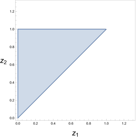
We are particularly interested in the boundary structure of the positive kinematic region since the boundary is where planar gauge theory amplitudes can have singularities Prlina:2018ukf; Arkani-Hamed:2019rds. This is most easily seen at tree level, where poles of the form $X_{i,j}\rightarrow 0$ manifestly correspond to boundaries of the region defined by eq. (3). Remarkably, not only singularities, but also possible branch cuts are encoded in the boundary structure of the positive kinematic region. However, the problem of finding distinct boundaries is more subtle than one might naively expect. Instead of investigating $Gr_{+}(4,n)/T$, let us consider a simpler version of the problem by studying the boundaries of $Gr_{+}(2,5)/T$. A naive parameterization of this space is

$$C_{i}^{\alpha}\sim\begin{pmatrix}1&1&1&1&0\\ 0&z_{1}&z_{2}&1&1\end{pmatrix}\ ,$$

(6)

where $0<z_{1}<z_{2}<1$ defines the positive region. We graph the positive region explicitly in fig. 1, where 3 boundaries are clearly manifest. However, let us now consider an alternative parameterization of the space with $u$-variables Arkani-Hamed:2019plo; Arkani-Hamed:2017mur; Arkani-Hamed:2020tuz

$$u_{i,j}=\frac{\langle i,j-1\rangle\langle i-1,j\rangle}{\langle i,j\rangle\langle i-1,j-1\rangle}\ ,$$

(7)

where $\langle a,b\rangle$ denotes a minor of $C_{i}^{\alpha}$. These $u_{i,j}$ variables obey the non-linear relations:

$$u_{1,3}=1-u_{2,4}u_{2,5},\quad(\textrm{Cyclic permutations}),$$

(8)

and the bounds, $0<u_{i,j}<1$, in the positive region. The second plot of the positive region in fig. 1 using $u$-variables shows that there are 5 boundaries, not 3. The underlying problem with eq. (6) is that a single set of coordinates, unless chosen very carefully, will not manifest all possible boundaries of the positive region. In other words, to study the boundary structure of the positive kinematic region, we need to study the compactified positive kinematic region, $\overline{Gr(4,n)/T}$.

Previous research into the connection between the positive kinematic region and $\mathcal{N}=4$ pSYM amplitudes has generally focused on the cluster algebra structure of the positive kinematic region Dixon:2011nj; Golden:2013xva; Golden:2013lha; Dixon:2013eka; Golden:2014pua; Golden:2014xqa; Drummond:2014ffa; Dixon:2014iba; Dixon:2014voa; Dixon:2015iva; Caron-Huot:2016owq; Drummond:2018caf; Caron-Huot:2019vjl; Caron-Huot:2019bsq.⁵⁵ 5 Note that alternate approaches have also been very successful without directly referencing the cluster algebra structure of the positive kinematic region. The $\bar{\mathcal{Q}}$ approach in particular has been extremely useful in probing $n\geq 8$ higher loop amplitudes CaronHuot:2011kk; Zhang:2019vnm; He:2020vob. Computations with irrational Yangian invariants provide a very clever probe of the algebraic letters He:2020uhb; Mago:2020kmp; Mago:2020nuv. Finally, studying branch points using Landau-equations and the amplitudhedron have allowed direct computations of the singularity structure at high loop order Dennen:2016mdk; Prlina:2017azl; Prlina:2017tvx. More concretely, the positive kinematic region of MHV $\mathcal{N}=4$ pSYM amplitudes corresponds to a $\mathcal{X}$-type cluster algebra⁶⁶ 6 A quick introduction to cluster algebras is provided in appendix A. which associates to the positive kinematic region a set of critically positive coordinates called $\hat{y}$-variables. A coordinate that is critically positive vanishes on at least one boundary of the positive region. Although each cluster parameterization makes only a sub-set of boundaries manifest, considering all cluster parameterizations together allows one to study all the possible boundaries. At 6-point and 7-point, the symbol alphabet, the $\phi_{i}$ in eq. (1), consists solely of the $\hat{y}$-variables, implying that $\hat{y}$-variables correspond to logarithmic branch cuts! Calculations are further simplified by considering a minimal multiplicative basis of $\hat{y}$-variables instead of the set of $\hat{y}$-variables themselves. Given an initial cluster, one minimal multiplicative basis consists of the $\hat{y}$-variables of an initial cluster, $\hat{y}_{i}$, along with some non-factorable Laurent polynomials of $\hat{y}_{i}$. We denote this set of non-factorable Laurent polynomials as $\mathcal{O}(\mathcal{X})$.

Starting at 8-point, two problematic features appear in the cluster algebra approach:

• •

  There are an infinite number of $\hat{y}$-variables in the cluster algebra.

• •

  Algebraic letters start to appear in the symbol alphabet.

Several approaches to tackling these problems have appeared in the literature and significant progress has been made.

In this paper, we propose wall crossing, and scattering diagrams more specifically, as a useful framework to address these issues Kontsevich:2013rda; 2007math……3822G; 2004math……6564K; 2018arXiv180605094R; 2017arXiv171206968R; 2014arXiv1411.1394G. Wall crossing has found applications in a number of research areas, such as the moduli spaces of $\mathcal{N}=2$ gauge theories and black hole entropy formulas Gaiotto:2009hg; Gaiotto:2010be; Andriyash:2010qv; Manschot:2010qz; Cordova:2013bza; Gaiotto:2015aoa. However, we are not studying any kind of entropy formula or moduli space, but instead compactifications of the positive kinematic region, $\overline{Gr(4,n)/T}$. The application of wall crossing and scattering diagrams to partial compactifications is best understood in the context of mirror symmetry 2011arXiv1106.4977G; Kontsevich:2013rda; 2014arXiv1411.1394G, but such a discussion is unfortunately beyond the scope of this paper.⁸⁸ 8 The schematic connection between mirror symmetry and cluster algebras is as follows. We can interpret $\mathcal{X}$ as the blow-up of an associated toric geometry. Cluster transformations correspond to changing the blow up description by an elementary transformation. Scattering diagrams provide a framework to systematically “sew” these different parameterizations together using a fan defined by tropical points of the dual mirror manifold, $\mathcal{A}^{\vee}$. This framework is famous for giving a geometric interpretation of the connection between tropical points of $\mathcal{A}^{\vee}$ and regular functions on $\mathcal{X}$ using mirror symmetry. Instead, we take a more practical approach, giving a computational definition of a scattering diagram with examples and then making the connection to cluster algebras. We argue that scattering diagrams, which represent a more general mathematical framework than cluster algebras, are useful for studying cluster algebraic functions that appear in the symbol alphabet of $\mathcal{N}=4$ pSYM.

A short introduction to cluster algebras is provided in appendix A. We restrict ourselves to cluster algebras whose exchange matrices are skew-symmetric, not just skew-symmetrizable. The techniques in this paper can be generalized to cluster algebras with non-skew-symmetric exchange matrices, but the formulas in this paper would require additional tweaking.

Notation: We denote the cluster variables associated with $\mathcal{A}$ and $\mathcal{X}$ as $x$ and $\hat{y}$ respectively. This notation differs from refs. Arkani-Hamed:2019rds; Henke:2019hve, which denote cluster variables associated with $\mathcal{A}$ and $\mathcal{X}$ as $a$ and $x$ respectively. Furthermore, we denote mutations of the $k$th node as $\mu_{k}$. For example, $x_{i}=\mu_{k}x_{i}$ if $i\neq k$. Finally, we often denote cluster algebras using the notation $A_{p_{1},p_{2},\ldots,p_{n}}$, because these cluster algebras correspond to the Teichmuller space of bordered Riemann surfaces. The cluster algebra $A_{p_{1},p_{2},\ldots,p_{n}}$ corresponds to the Teichmuller space of a Riemann surface with $n$ borders and $p_{i}$ punctures on border $i$. For those unfamiliar with the connection between cluster algebra and surfaces, this notation is unimportant for our applications to $\mathcal{N}=4$ pSYM but is nice for organizational purposes.

Our goal is to find a minimal multiplicative basis of the $\hat{y}$-variables that parameterize the positive region of $\mathcal{X}$. Unfortunately, the set of $\hat{y}$-variables is very difficult to study for a cluster algebra with generic frozen variables. For example, $\hat{y}$-variables will not always be independent. To see the problem, consider the initial quiver,

so

$$\hat{y}_{1}=\frac{1}{x_{2}},\quad\hat{y}_{2}=x_{1}x_{3},\quad\hat{y}_{3}=\frac{1}{x_{2}}\ .$$

(9)

Without any frozen nodes, we trivially see that $\hat{y}_{1}=\hat{y}_{3}$. However, suppose we include the frozen node

so $\hat{y}_{1}=y_{1}/x_{2}$ and $\hat{y}_{1}\neq\hat{y}_{3}$. From this example, it is clear that the frozen nodes play a crucial role in distinguishing $\hat{y}$-variables. One approach to this problem is to simply add frozen nodes until the $\hat{y}$-variables are maximally disambiguated 2006math……2259F; 2018arXiv180302492S. Only a finite, albeit large, number of frozen nodes are necessary to maximally disambiguate the $\hat{y}$-variables.

However, we are not interested in the set of all $\hat{y}$-variables but instead finding a multiplicatively independent basis. Given that any $\hat{y}$-variable can be written as a monomial of $x$-variables, we only need to maximally disambiguate $x$-variables of the cluster algebra, not the $\hat{y}$-variables. We are therefore motivated to consider a cluster algebra with a principal quiver 2006math……2259F. To construct a principal quiver, consider an initial quiver without any frozen nodes. Then add a frozen node, $y_{i}$, to each non-frozen node, $x_{i}$, with an edge pointing from the frozen node to the mutable node. For example, the quiver

(10)

is a principle quiver of the $A_{2}$ cluster algebra. Remarkably, the frozen nodes of a principal quiver are enough to maximally disambiguate all $x$-variables! Details of this statement are provided in appendix B. We subsequently study cluster algebras with principle quivers to study the multiplicative basis of $\hat{y}$-variables of cluster algebras with arbitrary frozen nodes. Furthermore, we can choose any quiver of our cluster algebra to be the principal quiver.

We now turn to the problem of understanding the relation between $\hat{y}$-variables and $x$-variables for a cluster algebra with a principal quiver. Although we cannot write a direct map from $\hat{y}$ to $x$, attempting to do so allows us to associate a canonical vector to each $x$-variable. Suppose we start with the principal quiver. Any $x$-variable in the cluster algebra can be written as a Laurent polynomial of the $x$-variables and $y$-variables of the principle quiver. It is not generally possible to re-write this Laurent polynomial entirely in terms of $\hat{y}$-variables. However, it can be written as a polynomial of $\hat{y}$-variables of the principle quiver up to a monomial of $x$-variables of the principle quiver:

$$x=x^{\vec{g}}F(\hat{y}_{i}),\quad x^{\vec{g}}=\prod_{i}x_{i}^{g_{i}}\ ,$$

(11)

where $F(\hat{y}_{i})$ is a Laurent polynomial in $\hat{y}$-variables of the principal quiver, which we denote as $\hat{y}_{i}$. No two $x$-variables share the same $g$-vector, allowing us to associate a canonical $g$-vector to each element of the cluster algebra. As an illustrative example, again consider the $A_{2}$ cluster algebra. The $\hat{y}$-variables of (10) are

$$\hat{y}_{1}=y_{1}x_{2}^{-1},\quad\hat{y}_{2}=y_{2}x_{1}\ .$$

(12)

Upon mutating $x_{1}$, we find

$$\begin{split}x_{3}&=\frac{y_{1}+x_{2}}{x_{1}}=\frac{x_{2}}{x_{1}}(1+\hat{y}_{1})\\ &\rightarrow\ \vec{g}=(-1,1),\quad F(\hat{y}_{i})=1+\hat{y}_{1}\ .\end{split}$$

(13)

Mutating through all clusters yields all $F(\hat{y}_{i})$ polynomials and $g$-vectors of the $A_{2}$ cluster algebra, which are provided in table 1. Each cluster defines a cone bounded by the $g$-vectors of the $x$-variables in the cluster. Remarkably, the cones associated with distinct clusters are nonoverlapping, which is not at all obvious from the above definition. The collection of these cones defines a (sometimes incomplete) fan.

• •

  A collection of cones bounded by co-dimension 1 walls. Each wall in the scattering diagram is associated with a scalar function, $f(y)$.

• •

  $N$ coordinates on $\mathcal{X}$, denoted as $\hat{y}_{\gamma_{i}}$. Each coordinate corresponds to a basis vector.¹⁰¹⁰ 10 We use the notation $\hat{y}_{\gamma_{i}}$, instead of $\hat{y}_{i}$, to distinguish them from $\hat{y}$-variables.

• •

  A skew-symmetric matrix, $B_{i,j}^{0}$, that defines a skew-symmetric¹¹¹¹ 11 The scattering diagram framework can also be applied when the product is skew-symmetrizable instead of just skew-symmetric, but the following formulas requires modifications. See ref. Gaiotto:2010be. product for the $\gamma$,

  $$\langle\gamma_{i},\gamma_{j}\rangle=\gamma_{i}\cdot B^{0}\cdot\gamma_{j}\ .$$

  (14)

Each cone in the fan is associated with a particular parameterization of $\mathcal{X}$ similar to how the $\hat{y}$-variables of a cluster correspond to a particular parameterization of $\mathcal{X}$. Crossing a wall between two cones corresponds to a coordinate transformation.

We now describe the coordinate transformation. Each co-dimension one wall is associated with a vector, $\gamma^{\perp}$, perpendicular to the wall,

$$\gamma^{\perp}=a_{i}\gamma_{i}\ .$$

(15)

The sign of $\gamma^{\perp}$ is chosen so $\gamma^{\perp}$ points opposite the direction one is mutating across the wall. Furthermore, the magnitude of $\gamma^{\perp}$ is chosen so that all of its components, the $a_{i}$ in eq. (15), are integers whose least common denominator is 1. Finally, we associate a unique monomial, $\hat{y}_{\gamma^{\perp}}$, to each $\gamma^{\perp}$:

	$\displaystyle\hat{y}_{\gamma^{\perp}}$	$\displaystyle=(\prod\hat{y}_{\gamma_{i}}^{a_{i}})^{\textrm{Sign}(\gamma^{\perp}\cdot\vec{N})}\ ,$		(16)
	$\displaystyle\vec{N}$	$\displaystyle=(1,1,\ldots,1)\ .$		(17)

For example, for a wall with the perpendicular vector $\gamma^{\perp}=(0,\ 1,\ 1)$, the associated monomial is

$$\begin{split}\hat{y}_{(0,\ 1,\ 1)}=\hat{y}_{\gamma_{2}}\hat{y}_{\gamma_{3}}\ .\end{split}$$

(18)

Due to the $\textrm{Sign}(\gamma^{\perp}\cdot\vec{N})$ exponent, the perpendicular vector $\gamma^{\perp}=(0,\ -1,\ -1)$ is associated with the same monomial,

$$\begin{split}\hat{y}_{(0,\ -1,\ -1)}=\hat{y}_{\gamma_{2}}\hat{y}_{\gamma_{3}}\ .\end{split}$$

(19)

This makes sense as $(0,\ -1,\ -1)$ and $(0,\ 1,\ 1)$ correspond to the same wall and should therefore be associated with the same monomial. Although $\gamma^{\perp}$ flips sign depending on the direction you are mutating across the wall, $\hat{y}_{\gamma^{\perp}}$ is the same due to the $\textrm{Sign}(\gamma^{\perp}\cdot\vec{N})$ exponent. The mutation relation for $\hat{y}_{\gamma_{i}}$ across a wall is

$$\hat{y}_{\gamma_{i}}\rightarrow\hat{y}_{\gamma_{i}}f(\hat{y}_{\gamma^{\perp}})^{\langle\gamma_{i},\gamma^{\perp}\rangle}\ ,$$

(20)

which gives the $\hat{y}_{\gamma_{i}}$ of the new cone in terms of $\hat{y}_{\gamma_{i}}$ of the initial cone. To see eq. (20) in an explicit example, suppose we are crossing from cone $C_{1}$ to cone $C_{2}$ in fig. 4(a), where we fix,

$$B^{0}_{i,j}=\begin{bmatrix}0&1\\ -1&0\end{bmatrix}\ ,$$

(21)

and $f(y)=1+y$ for all walls. The perpendicular vector for the relevant wall is $\gamma^{\perp}=(0,1)$, so $\hat{y}_{\gamma^{\perp}}=\hat{y}_{\gamma_{2}}$. Applying eq. (20), the $\hat{y}_{\gamma_{i}}$ of chamber $C_{2}$ are then

$$\begin{split}\hat{y}_{\gamma_{1}}&=\hat{y}_{\gamma_{1}}^{\text{I}}(1+\hat{y}_{\gamma_{2}}^{\text{I}})^{(1,0)\cdot B^{0}\cdot(0,1)}=\hat{y}_{\gamma_{1}}^{\text{I}}(1+\hat{y}_{\gamma_{2}}^{\text{I}})\ ,\\ \hat{y}_{\gamma_{2}}&=\hat{y}_{\gamma_{2}}^{\text{I}}(1+\hat{y}_{\gamma_{2}}^{\text{I}})^{(0,1)\cdot B^{0}\cdot(0,1)}=\hat{y}_{\gamma_{2}}^{\text{I}}\ ,\\ \end{split}$$

(22)

where $\hat{y}_{\gamma_{i}}^{\text{I}}$ corresponds to the $\hat{y}_{\gamma_{i}}$ of cone $C_{1}$.

For a scattering diagram to be self-consistent, the relations between the $\hat{y}_{\gamma_{i}}$ of any two cones should be path independent. To see why self-consistency is non-trivial, again consider the scattering diagram in fig. 4(a) with the same $B_{i,j}^{0}$ and $f(y)$. Applying eq. (20) to each path in fig. 4(a), we find

	$\displaystyle\begin{pmatrix}\hat{y}^{\text{I}}_{\gamma_{1}}\\ \hat{y}^{\text{I}}_{\gamma_{2}}\end{pmatrix}$	$\displaystyle\rightarrow\begin{pmatrix}\hat{y}^{\text{I}}_{\gamma_{1}}\\ \frac{\hat{y}^{\text{I}}_{\gamma_{2}}}{\hat{y}^{\text{I}}_{\gamma_{1}}+1}\end{pmatrix}\rightarrow\begin{pmatrix}\hat{y}^{\text{I}}_{\gamma_{1}}\left(\frac{\hat{y}^{\text{I}}_{\gamma_{2}}}{\hat{y}^{\text{I}}_{\gamma_{1}}+1}+1\right)\\ \frac{\hat{y}^{\text{I}}_{\gamma_{2}}}{\hat{y}^{\text{I}}_{\gamma_{1}}+1}\end{pmatrix}\ ,$
	$\displaystyle\begin{pmatrix}\hat{y}^{\text{I}}_{\gamma_{1}}\\ \hat{y}^{\text{I}}_{\gamma_{2}}\end{pmatrix}$	$\displaystyle\rightarrow\begin{pmatrix}\hat{y}^{\text{I}}_{\gamma_{1}}\left(\hat{y}^{\text{I}}_{\gamma_{2}}+1\right)\\ \hat{y}^{\text{I}}_{\gamma_{2}}\end{pmatrix}\rightarrow\begin{pmatrix}\hat{y}^{\text{I}}_{\gamma_{1}}\left(\hat{y}^{\text{I}}_{\gamma_{2}}+1\right)\\ \frac{\hat{y}^{\text{I}}_{\gamma_{2}}}{\hat{y}^{\text{I}}_{\gamma_{1}}\left(\hat{y}^{\text{I}}_{\gamma_{2}}+1\right)+1}\end{pmatrix}\ ,$		(23)

where $\hat{y}^{\text{I}}_{\gamma_{i}}$ again corresponds to the $\hat{y}_{\gamma_{i}}$ of the initial cone, $C_{1}$. The scattering diagram in fig. 4(a) is inconsistent as the $\hat{y}_{\gamma_{i}}$ associated with $C_{3}$ are not path independent. To make the scattering diagram self-consistent, we must include the additional wall $\gamma^{\perp}=(1,1)$, leading to the scattering diagram in fig. 4(b). Including this second wall, the first line in eq. (23) becomes

$$\begin{split}\begin{pmatrix}\hat{y}^{\text{I}}_{\gamma_{1}}\\ \hat{y}^{\text{I}}_{\gamma_{2}}\end{pmatrix}\rightarrow\begin{pmatrix}\hat{y}^{\text{I}}_{\gamma_{1}}\\ \frac{\hat{y}^{\text{I}}_{\gamma_{2}}}{\hat{y}^{\text{I}}_{\gamma_{1}}+1}\end{pmatrix}\rightarrow\begin{pmatrix}\hat{y}^{\text{I}}_{\gamma_{1}}\left(\frac{\hat{y}^{\text{I}}_{\gamma_{1}}\hat{y}^{\text{I}}_{\gamma_{2}}}{\hat{y}^{\text{I}}_{\gamma_{1}}+1}+1\right)\\ \frac{\hat{y}^{\text{I}}_{\gamma_{2}}}{\hat{y}^{\text{I}}_{\gamma_{1}}\left(\hat{y}^{\text{I}}_{\gamma_{2}}+1\right)+1}\end{pmatrix}\rightarrow\begin{pmatrix}\hat{y}^{\text{I}}_{\gamma_{1}}\left(\hat{y}^{\text{I}}_{\gamma_{2}}+1\right)\\ \frac{\hat{y}^{\text{I}}_{\gamma_{2}}}{\hat{y}^{\text{I}}_{\gamma_{1}}\left(\hat{y}^{\text{I}}_{\gamma_{2}}+1\right)+1}\end{pmatrix}\ ,\end{split}$$

(24)

which now matches the second line of eq. (23).

We now describe the connection between cluster algebras and scattering diagrams. The relation between scattering diagrams and cluster algebras is that the $g$-vector fan defines a scattering diagram where each cluster is dual to a cone in the scattering diagram. The $B_{i,j}^{0}$ matrix that defines the skew-symmetric product in eq. (14) corresponds to the exchange matrix of the principal quiver. For a cluster algebra with a finite number of cones, each wall corresponds to a cluster mutation and we fix

$$f(y)=1+y$$

(25)

for all walls. We call the walls that correspond to cluster mutations, cluster walls. The $\hat{y}$-variables of a given cone are the $\hat{y}_{\gamma^{\perp}}$ associated with each wall that bounds the cone,

$$\hat{y}_{j}=\prod\hat{y}_{\gamma_{i}}^{a_{i}^{j}},\quad\gamma^{\perp}_{j}=a_{i}^{j}\gamma_{i}\ ,$$

(26)

where $\gamma^{\perp}_{i}$ is the $\gamma^{\perp}$ associated with $\hat{y}_{i}$. Note that $\gamma^{\perp}_{j}$ points inward from the cone in this convention. Furthermore, the exchange matrix of the quiver associated with a cone is

$$B_{i,j}=\langle\gamma^{\perp}_{i},\gamma^{\perp}_{j}\rangle\ .$$

(27)

For example, for the cone associated with the principle quiver, the principle cone, we have

$$\begin{split}\gamma_{i}^{\perp}|_{\textrm{Principle Cone}}&=\gamma_{i}\end{split}$$

(28)

so

$$\hat{y}_{\gamma_{i}}|_{\textrm{Principle Cone}}=\hat{y}_{i},\quad B_{i,j}|_{\textrm{Principle Cone}}=\gamma_{i}\cdot B^{0}\cdot\gamma_{j}=B_{i,j}^{0}\ .$$

(29)

The cluster mutation in eq. (94) corresponds to both a wall crossing transform, eq. (20), and a mutation in the $\gamma^{\perp}_{i}$. To see this, again consider the cluster algebra associated with the quiver

The explicit computation of the $g$-vectors in table 1 reveals that it is the same as fig. 4(b). Consider a mutation from cone $C_{1}$ to $C_{2}$. The $\hat{y}_{\gamma_{i}}$ mutation is given by eq. (22) and the $\gamma_{i}^{\perp}$ mutate as

$$\begin{split}\gamma^{\perp}_{1}=(1,0)&\rightarrow\gamma^{\perp}_{1}=(1,0)\ ,\\ \gamma^{\perp}_{2}=(0,1)&\rightarrow\gamma^{\perp}_{2}=(0,-1)\ .\end{split}$$

(30)

Combining eqs. (22) and (30), the mutation relation for $\hat{y}_{i}$ is

$$\begin{pmatrix}\hat{y}_{1}\\ \hat{y}_{2}\end{pmatrix}\rightarrow\begin{pmatrix}\hat{y}_{1}(1+\hat{y}_{2})\\ \frac{1}{\hat{y}_{2}}\end{pmatrix}\ ,$$

(31)

which exactly matches the mutation relation for $\hat{y}$-variables. Again, note that it was a combination of mutating $\gamma_{i}^{\perp}$ and $\hat{y}_{\gamma_{i}}$ that gave the cluster mutation relation for the $\hat{y}$-variables.

We can also consider the scattering diagrams of more complex cluster algebras, such as the $A_{3}$ cluster algebra

which is associated with $\overline{Gr(2,6)/T}$. Since the cluster algebra is rank 3, the associated scattering diagram is 3 dimensional. From direct calculation, we found the scattering diagram given in fig. 2 in the Introduction. The walls are now 2 dimensional and defined by the span of two $g$-vectors. To find the wall associated with the $\hat{y}$-variable of a specific quiver, consider all the $g$-vectors bounding the dual cone except the $g$-vector of the $x$ variable associated with the same node as the $\hat{y}$-variable. The span of these two $g$-vectors defines the wall associated with the $\hat{y}$-variable.

We first show that the $g$-vector fans of infinite cluster algebras need to include additional walls that do not correspond to cluster mutations. Furthermore, we will find the functions attached to these walls are not elements of the cluster algebra and can be identified with the mysterious cluster algebraic functions of ref. Arkani-Hamed:2019rds. We will study the cluster algebra defined by the principal quiver

as our motivating example. A review of relevant derivations and formulas for this cluster algebra are provided in appendix C. The key results are a closed form solution for $x_{i}$ with $i>0$,

$$\begin{split}x_{i}&=\frac{1}{2^{i+2}}[(x_{-1}+B_{+}\sqrt{\triangle})(\mathcal{P}+\sqrt{\triangle})^{i+1}+(x_{-1}-B_{+}\sqrt{\triangle})(\mathcal{P}-\sqrt{\triangle})^{i+1}]\ ,\\ &\quad\mathcal{P}=\frac{y_{-1}}{x_{-1}x_{0}}+\frac{x_{0}}{x_{-1}}+\frac{x_{-1}y_{-1}y_{0}}{x_{0}}\ ,\\ &\quad B_{+}=\frac{2x_{0}-x_{-1}\mathcal{P}}{\triangle}\ ,\\ &\quad\triangle=\mathcal{P}^{2}-4y_{-1}y_{0}\ ,\end{split}$$

(32)

and an equation for $\hat{y}_{2n-1}$ and $\hat{y}_{2n}$ in terms of $x$-variables after $2n$ mutations,

$$\hat{y}_{2n-1}=y_{0}^{n}y_{-1}^{2n+1}x_{2n}^{-2},\quad\hat{y}_{2n}=y_{0}^{1-2n}y_{-1}^{-2n}x_{2n-1}^{2}\ .$$

(33)

The $g$-vectors, denoted by black arrows in fig. 5, are

$$\vec{g}_{i}=\left\{\begin{matrix}(-i,i+1)&i\geq-1\\ (2+i,-i-3)&i\leq-2\end{matrix}\right.\ .$$

(34)

We will now show that the self-consistency of the scattering diagram requires the existence of a new wall associated with the limiting ray that does not correspond to a standard cluster mutation.

Consider cones that are asymptotically close to the limiting ray. Importantly, the $\hat{y}_{i}$ variables go to $0$ or $\infty$ as we approach the limiting ray, which can be seen from eqs. (32) and (33). To calculate $\hat{y}_{\gamma_{i}}$ in this limit, we first express $\hat{y}_{\gamma_{i}}$ in terms of monomials of $\hat{y}$-variables. From the scattering diagram in fig. 5, the $\gamma^{\perp}_{i}$ associated with the $\hat{y}_{i}$ in eq. (33) are

$$[\gamma_{-1}^{\perp}]^{2n}=(1+2n,2n),\quad[\gamma_{0}^{\perp}]^{2n}=(-2n,1-2n)\ ,$$

(35)

where $[\gamma_{i}^{\perp}]^{2n}$ is the perpendicular vector to the wall associated with node $x_{i}$ after $2n$ mutations. We subsequently found that

$$\begin{split}\gamma_{1}&=(1-2n)[\gamma_{-1}^{\perp}]^{2n}-2n[\gamma_{0}^{\perp}]^{2n}\ ,\\ \gamma_{2}&=2n[\gamma_{-1}^{\perp}]^{2n}+(2n+1)[\gamma_{0}^{\perp}]^{2n}\ .\end{split}$$

(36)

Combining eqs. (26) and (36) gives a formula for $\hat{y}_{\gamma_{i}}$ in the asymptotic limit, denoted as $\hat{y}_{\gamma_{i}}^{+}$,

$$\begin{split}\hat{y}_{\gamma_{1}}^{+}&=\lim_{n\rightarrow\infty}(\hat{y}_{2n-1})^{1-2n}(\hat{y}_{2n})^{-2n}=16y_{-1}(x_{-1}+B_{+}\sqrt{\triangle})^{-2}(\mathcal{P}+\sqrt{\triangle})^{-2}\ ,\\ \hat{y}_{\gamma_{2}}^{+}&=\lim_{n\rightarrow\infty}(\hat{y}_{2n-1})^{2n}(\hat{y}_{2n})^{2n+1}=\frac{y_{0}}{4}(x_{-1}+B_{+}\sqrt{\triangle})^{2}\ .\end{split}$$

(37)

We used the explicit formulas for $\hat{y}_{i}$ in eqs. (32) and (33) to write the final expressions for $\hat{y}_{\gamma_{1}}^{+}$ and $\hat{y}_{\gamma_{2}}^{+}$ in terms of our initial cluster variables: $y_{-1}$, $y_{0}$, $x_{-1}$ and $x_{0}$. The final expressions in eq. (37) are finite and provide a multiplicative basis for the $\hat{y}$-variables asymptotically close to the limiting wall if one approaches from the right. A visualization of the path is given by the green line in fig. 6.

We then repeated the same calculation, but following the blue line in fig. 6. If one approaches from the left, the asymptotic limits of $\hat{y}_{\gamma_{i}}$, denoted as $\hat{y}_{\gamma_{i}}^{-}$, are

$$\begin{split}\hat{y}_{\gamma_{1}}^{-}&=\hat{y}_{\gamma_{1}}^{+}(1-\frac{\mathcal{P}-\sqrt{\mathcal{P}^{2}-4y_{-1}y_{0}}}{\mathcal{P}+\sqrt{\mathcal{P}^{2}-4y_{-1}y_{0}}})^{-4}\ ,\\ \hat{y}_{\gamma_{2}}^{-}&=\hat{y}_{\gamma_{2}}^{+}(1-\frac{\mathcal{P}-\sqrt{\mathcal{P}^{2}-4y_{-1}y_{0}}}{\mathcal{P}+\sqrt{\mathcal{P}^{2}-4y_{-1}y_{0}}})^{4}\ .\end{split}$$

(38)

The fact that eqs. (37) and (38) are not equal indicates that the scattering diagram must include another wall to be self-consistent. However, eq. (38) can be re-written into the suggestive form

$$\hat{y}_{\gamma_{i}}^{-}=\hat{y}_{\gamma_{i}}^{+}(1-\hat{y}_{\gamma^{\perp}})^{-2\langle\gamma_{i},\gamma^{\perp}\rangle},\quad\hat{y}_{\gamma^{\perp}}=\hat{y}_{\gamma_{1}}^{+}\hat{y}_{\gamma_{2}}^{+}=\hat{y}_{\gamma_{1}}^{-}\hat{y}_{\gamma_{2}}^{-},\quad\gamma^{\perp}=(1,1)\ ,$$

(39)

which can be matched to eq. (20) by requiring $f(\hat{y})=(1-\hat{y})^{-2}$. Eq. (39) shows that we must include a limiting wall with $\gamma^{\perp}=(1,1)$ for the scattering diagram to be self-consistent. The $\hat{y}_{\gamma^{\perp}}$ associated with the limiting wall,

$$\begin{split}\hat{y}_{\gamma^{\perp}}&=\hat{y}_{\gamma_{1}}^{+}\hat{y}_{\gamma_{2}}^{+}\ ,\\ &=\frac{\mathcal{P}-\sqrt{\mathcal{P}^{2}-4y_{-1}y_{0}}}{\mathcal{P}+\sqrt{\mathcal{P}^{2}-4y_{-1}y_{0}}}\ ,\end{split}$$

(40)

takes exactly the right form for eq. (39) to be matched with eq. (20). The limiting wall corresponds to the red line in figs. 5 and 6. Performing a mutation across this limiting wall cannot be identified with a cluster mutation in the $A_{1,1}$ scattering diagram. From the perspective of the cluster algebra, these cones are separated by an infinite number of cluster mutations. Finally, the $\hat{y}_{\gamma^{\perp}}$ of the limiting wall obeys the bound $0<\hat{y}_{\gamma^{\perp}}<1$ in contrast to normal $\hat{y}$-variables which are just positive definite.

References

- (1) J. Drummond, J. Foster, O. Gürdogan and C. Kalousios, Algebraic singularities of scattering amplitudes from tropical geometry, JHEP 04 (2021) 002, [1912.08217].
- (2) Z. Bern, J. J. M. Carrasco and H. Johansson, Perturbative Quantum Gravity as a Double Copy of Gauge Theory, Phys. Rev. Lett. 105 (2010) 061602, [1004.0476].
- (3) Z. Bern, J. J. Carrasco, M. Chiodaroli, H. Johansson and R. Roiban, The Duality Between Color and Kinematics and its Applications, 1909.01358.
- (4) Z. Bern, C. Cheung, R. Roiban, C.-H. Shen, M. P. Solon and M. Zeng, Black Hole Binary Dynamics from the Double Copy and Effective Theory, JHEP 10 (2019) 206, [1908.01493].
- (5) N. Arkani-Hamed, Y. Bai, S. He and G. Yan, Scattering Forms and the Positive Geometry of Kinematics, Color and the Worldsheet, JHEP 05 (2018) 096, [1711.09102].
- (6) N. Arkani-Hamed, Y. Bai and T. Lam, Positive Geometries and Canonical Forms, JHEP 11 (2017) 039, [1703.04541].
- (7) N. Arkani-Hamed, S. He and T. Lam, Stringy canonical forms, JHEP 02 (2021) 069, [1912.08707].
- (8) S. Mizera, Scattering Amplitudes from Intersection Theory, Phys. Rev. Lett. 120 (2018) 141602, [1711.00469].
- (9) P. Mastrolia and S. Mizera, Feynman Integrals and Intersection Theory, JHEP 02 (2019) 139, [1810.03818].
- (10) S. Mizera, Status of Intersection Theory and Feynman Integrals, 2002.10476.
- (11) H. Elvang and Y.-t. Huang, Scattering Amplitudes, 1308.1697.
- (12) N. Arkani-Hamed, T.-C. Huang and Y.-t. Huang, Scattering Amplitudes For All Masses and Spins, 1709.04891.
- (13) M.-Z. Chung, Y.-T. Huang, J.-W. Kim and S. Lee, The simplest massive S-matrix: from minimal coupling to Black Holes, JHEP 04 (2019) 156, [1812.08752].
- (14) D. Chicherin, J. M. Henn and G. Papathanasiou, Cluster algebras for Feynman integrals, Phys. Rev. Lett. 126 (2021) 091603, [2012.12285].
- (15) H. Elvang, Bootstrap and Amplitudes: A Hike in the Landscape of Quantum Field Theory, 2007.08436.
- (16) H. Elvang, M. Hadjiantonis, C. R. Jones and S. Paranjape, Soft Bootstrap and Supersymmetry, JHEP 01 (2019) 195, [1806.06079].
- (17) Z. Bern, A. Luna, R. Roiban, C.-H. Shen and M. Zeng, Spinning Black Hole Binary Dynamics, Scattering Amplitudes and Effective Field Theory, 2005.03071.
- (18) J. Trnka, Towards the Gravituhedron: New Expressions for NMHV Gravity Amplitudes, JHEP 04 (2021) 253, [2012.15780].
- (19) Z. Bern and Y.-t. Huang, Basics of Generalized Unitarity, J. Phys. A 44 (2011) 454003, [1103.1869].
- (20) J. L. Bourjaily, E. Herrmann and J. Trnka, Prescriptive Unitarity, JHEP 06 (2017) 059, [1704.05460].
- (21) J. L. Bourjaily, E. Herrmann, C. Langer, A. J. McLeod and J. Trnka, Prescriptive Unitarity for Non-Planar Six-Particle Amplitudes at Two Loops, JHEP 12 (2019) 073, [1909.09131].
- (22) A. Adams, N. Arkani-Hamed, S. Dubovsky, A. Nicolis and R. Rattazzi, Causality, analyticity and an IR obstruction to UV completion, JHEP 10 (2006) 014, [hep-th/0602178].
- (23) X. O. Camanho, J. D. Edelstein, J. Maldacena and A. Zhiboedov, Causality Constraints on Corrections to the Graviton Three-Point Coupling, JHEP 02 (2016) 020, [1407.5597].
- (24) N. Arkani-Hamed, T.-C. Huang and Y.-T. Huang, The EFT-Hedron, JHEP 05 (2021) 259, [2012.15849].
- (25) S. Caron-Huot and V. Van Duong, Extremal Effective Field Theories, JHEP 05 (2021) 280, [2011.02957].
- (26) T. Trott, Causality, Unitarity and Symmetry in Effective Field Theory, 2011.10058.
- (27) J. Drummond, J. Foster and O. Gürdoğan, Cluster Adjacency Properties of Scattering Amplitudes in Supersymmetric Yang-Mills Theory, Phys. Rev. Lett. 120 (2018) 161601, [1710.10953].
- (28) J. Drummond, J. Foster and O. Gurdogan, Cluster adjacency beyond MHV, JHEP 03 (2019) 086, [1810.08149].
- (29) J. L. Bourjaily, H. Hannesdottir, A. J. McLeod, M. D. Schwartz and C. Vergu, Sequential Discontinuities of Feynman Integrals and the Monodromy Group, 2007.13747.
- (30) L. F. Alday, D. Gaiotto and J. Maldacena, Thermodynamic Bubble Ansatz, JHEP 09 (2011) 032, [0911.4708].
- (31) S. Caron-Huot, L. J. Dixon, J. M. Drummond, F. Dulat, J. Foster, O. Gürdoğan et al., The Steinmann Cluster Bootstrap for = 4 Super Yang-Mills Amplitudes, PoS CORFU2019 (2020) 003, [2005.06735].
- (32) N. Arkani-Hamed, T. Lam and M. Spradlin, Non-perturbative geometries for planar SYM amplitudes, 1912.08222.
- (33) J. Golden, A. B. Goncharov, M. Spradlin, C. Vergu and A. Volovich, Motivic Amplitudes and Cluster Coordinates, JHEP 01 (2014) 091, [1305.1617].
- (34) J. Golden and M. Spradlin, The differential of all two-loop MHV amplitudes in = 4 Yang-Mills theory, JHEP 09 (2013) 111, [1306.1833].
- (35) J. Golden, M. F. Paulos, M. Spradlin and A. Volovich, Cluster Polylogarithms for Scattering Amplitudes, J. Phys. A 47 (2014) 474005, [1401.6446].
- (36) I. Prlina, M. Spradlin, J. Stankowicz, S. Stanojevic and A. Volovich, All-Helicity Symbol Alphabets from Unwound Amplituhedra, JHEP 05 (2018) 159, [1711.11507].
- (37) I. Prlina, M. Spradlin, J. Stankowicz and S. Stanojevic, Boundaries of Amplituhedra and NMHV Symbol Alphabets at Two Loops, JHEP 04 (2018) 049, [1712.08049].
- (38) S. He, Z. Li and C. Zhang, Two-loop Octagons, Algebraic Letters and Equations, Phys. Rev. D 101 (2020) 061701, [1911.01290].
- (39) M. Kontsevich and Y. Soibelman, Wall-crossing structures in Donaldson-Thomas invariants, integrable systems and Mirror Symmetry, Lect. Notes Union. Mat. Ital. 15 (2014) 197–308, [1303.3253].
- (40) M. Gross and B. Siebert, From real affine geometry to complex geometry, arXiv Mathematics e-prints (Mar., 2007) math/0703822, [math/0703822].
- (41) M. Kontsevich and Y. Soibelman, Affine structures and non-archimedean analytic spaces, arXiv Mathematics e-prints (June, 2004) math/0406564, [math/0406564].
- (42) N. Reading, A combinatorial approach to scattering diagrams, arXiv e-prints (June, 2018) arXiv:1806.05094, [1806.05094].
- (43) N. Reading, Scattering fans, arXiv e-prints (Dec., 2017) arXiv:1712.06968, [1712.06968].
- (44) M. Gross, P. Hacking, S. Keel and M. Kontsevich, Canonical bases for cluster algebras, arXiv e-prints (Nov., 2014) arXiv:1411.1394, [1411.1394].
- (45) I. Prlina, M. Spradlin and S. Stanojevic, All-loop singularities of scattering amplitudes in massless planar theories, Phys. Rev. Lett. 121 (2018) 081601, [1805.11617].
- (46) N. Arkani-Hamed and J. Trnka, The Amplituhedron, JHEP 10 (2014) 030, [1312.2007].
- (47) N. Arkani-Hamed, H. Thomas and J. Trnka, Unwinding the Amplituhedron in Binary, JHEP 01 (2018) 016, [1704.05069].
- (48) E. Herrmann, C. Langer, J. Trnka and M. Zheng, Positive geometry, local triangulations, and the dual of the Amplituhedron, JHEP 01 (2021) 035, [2009.05607].
- (49) N. Arkani-Hamed, J. L. Bourjaily, F. Cachazo, A. B. Goncharov, A. Postnikov and J. Trnka, Grassmannian Geometry of Scattering Amplitudes. Cambridge University Press, 2016, 10.1017/CBO9781316091548.
- (50) R. Kojima and C. Langer, Sign Flip Triangulations of the Amplituhedron, JHEP 05 (2020) 121, [2001.06473].
- (51) C. Anastasiou, Z. Bern, L. J. Dixon and D. Kosower, Planar amplitudes in maximally supersymmetric Yang-Mills theory, Phys. Rev. Lett. 91 (2003) 251602, [hep-th/0309040].
- (52) Z. Bern, L. J. Dixon and V. A. Smirnov, Iteration of planar amplitudes in maximally supersymmetric Yang-Mills theory at three loops and beyond, Phys. Rev. D 72 (2005) 085001, [hep-th/0505205].
- (53) L. F. Alday and J. M. Maldacena, Gluon scattering amplitudes at strong coupling, JHEP 06 (2007) 064, [0705.0303].
- (54) G. Yang, A simple collinear limit of scattering amplitudes at strong coupling, JHEP 03 (2011) 087, [1006.3306].
- (55) A. Brandhuber, P. Heslop and G. Travaglini, MHV amplitudes in N=4 super Yang-Mills and Wilson loops, Nucl. Phys. B 794 (2008) 231–243, [0707.1153].
- (56) L. F. Alday, D. Gaiotto, J. Maldacena, A. Sever and P. Vieira, An Operator Product Expansion for Polygonal null Wilson Loops, JHEP 04 (2011) 088, [1006.2788].
- (57) S. Caron-Huot, Notes on the scattering amplitude / Wilson loop duality, JHEP 07 (2011) 058, [1010.1167].
- (58) B. Eden, P. Heslop, G. P. Korchemsky and E. Sokatchev, The super-correlator/super-amplitude duality: Part I, Nucl. Phys. B 869 (2013) 329–377, [1103.3714].
- (59) B. Basso, A. Sever and P. Vieira, Spacetime and Flux Tube S-Matrices at Finite Coupling for N=4 Supersymmetric Yang-Mills Theory, Phys. Rev. Lett. 111 (2013) 091602, [1303.1396].
- (60) S. He, Z. Li, Q. Yang and C. Zhang, Feynman Integrals and Scattering Amplitudes from Wilson Loops, Phys. Rev. Lett. 126 (2021) 231601, [2012.15042].
- (61) S. He, Z. Li, Y. Tang and Q. Yang, The Wilson-loop log representation for Feynman integrals, JHEP 05 (2021) 052, [2012.13094].
- (62) S. He, Z. Li and Q. Yang, Notes on cluster algebras and some all-loop Feynman integrals, 2103.02796.
- (63) A. B. Goncharov, M. Spradlin, C. Vergu and A. Volovich, Classical Polylogarithms for Amplitudes and Wilson Loops, Phys. Rev. Lett. 105 (2010) 151605, [1006.5703].
- (64) D. Gaiotto, J. Maldacena, A. Sever and P. Vieira, Pulling the straps of polygons, JHEP 12 (2011) 011, [1102.0062].
- (65) A. B. Goncharov, Multiple polylogarithms, cyclotomy and modular complexes, arXiv e-prints (May, 2011) arXiv:1105.2076, [1105.2076].
- (66) C. Duhr, Mathematical aspects of scattering amplitudes, in Theoretical Advanced Study Institute in Elementary Particle Physics: Journeys Through the Precision Frontier: Amplitudes for Colliders, pp. 419–476, 2015. 1411.7538. DOI.
- (67) A. Goncharov, Geometry of configurations, polylogarithms, and motivic cohomology, Advances in Mathematics 114 (1995) 197 – 318.
- (68) F. Brown and C. Duhr, A double integral of dlog forms which is not polylogarithmic, 2006.09413.
- (69) A. Sen, String Field Theory as World-sheet UV Regulator, JHEP 10 (2019) 119, [1902.00263].
- (70) E. Witten, The Feynman in String Theory, JHEP 04 (2015) 055, [1307.5124].
- (71) N. Arkani-Hamed, S. He, T. Lam and H. Thomas, Binary Geometries, Generalized Particles and Strings, and Cluster Algebras, 1912.11764.
- (72) N. Arkani-Hamed, S. He and T. Lam, Cluster configuration spaces of finite type, 2005.11419.
- (73) L. J. Dixon, J. M. Drummond and J. M. Henn, Analytic result for the two-loop six-point NMHV amplitude in N=4 super Yang-Mills theory, JHEP 01 (2012) 024, [1111.1704].
- (74) L. J. Dixon, J. M. Drummond, M. von Hippel and J. Pennington, Hexagon functions and the three-loop remainder function, JHEP 12 (2013) 049, [1308.2276].
- (75) J. Golden and M. Spradlin, A Cluster Bootstrap for Two-Loop MHV Amplitudes, JHEP 02 (2015) 002, [1411.3289].
- (76) J. M. Drummond, G. Papathanasiou and M. Spradlin, A Symbol of Uniqueness: The Cluster Bootstrap for the 3-Loop MHV Heptagon, JHEP 03 (2015) 072, [1412.3763].
- (77) L. J. Dixon and M. von Hippel, Bootstrapping an NMHV amplitude through three loops, JHEP 10 (2014) 065, [1408.1505].
- (78) L. J. Dixon, J. M. Drummond, C. Duhr and J. Pennington, The four-loop remainder function and multi-Regge behavior at NNLLA in planar N = 4 super-Yang-Mills theory, JHEP 06 (2014) 116, [1402.3300].
- (79) L. J. Dixon, M. von Hippel and A. J. McLeod, The four-loop six-gluon NMHV ratio function, JHEP 01 (2016) 053, [1509.08127].
- (80) S. Caron-Huot, L. J. Dixon, A. McLeod and M. von Hippel, Bootstrapping a Five-Loop Amplitude Using Steinmann Relations, Phys. Rev. Lett. 117 (2016) 241601, [1609.00669].
- (81) J. Drummond, J. Foster, O. Gürdoğan and G. Papathanasiou, Cluster adjacency and the four-loop NMHV heptagon, JHEP 03 (2019) 087, [1812.04640].
- (82) S. Caron-Huot, L. J. Dixon, F. Dulat, M. von Hippel, A. J. McLeod and G. Papathanasiou, Six-Gluon amplitudes in planar = 4 super-Yang-Mills theory at six and seven loops, JHEP 08 (2019) 016, [1903.10890].
- (83) S. Caron-Huot, L. J. Dixon, F. Dulat, M. Von Hippel, A. J. McLeod and G. Papathanasiou, The Cosmic Galois Group and Extended Steinmann Relations for Planar SYM Amplitudes, JHEP 09 (2019) 061, [1906.07116].
- (84) S. Caron-Huot and S. He, Jumpstarting the All-Loop S-Matrix of Planar N=4 Super Yang-Mills, JHEP 07 (2012) 174, [1112.1060].
- (85) S. He, Z. Li and C. Zhang, The symbol and alphabet of two-loop NMHV amplitudes from equations, JHEP 03 (2021) 278, [2009.11471].
- (86) S. He and Z. Li, A note on letters of Yangian invariants, JHEP 02 (2021) 155, [2007.01574].
- (87) J. Mago, A. Schreiber, M. Spradlin and A. Volovich, Symbol alphabets from plabic graphs, JHEP 10 (2020) 128, [2007.00646].
- (88) J. Mago, A. Schreiber, M. Spradlin, A. Yelleshpur Srikant and A. Volovich, Symbol alphabets from plabic graphs II: rational letters, JHEP 04 (2021) 056, [2012.15812].
- (89) T. Dennen, I. Prlina, M. Spradlin, S. Stanojevic and A. Volovich, Landau Singularities from the Amplituhedron, JHEP 06 (2017) 152, [1612.02708].
- (90) S. He, L. Ren and Y. Zhang, Notes on polytopes, amplitudes and boundary configurations for Grassmannian string integrals, JHEP 04 (2020) 140, [2001.09603].
- (91) N. Arkani-Hamed, T. Lam and M. Spradlin, Positive configuration space, 2003.03904.
- (92) N. Henke and G. Papathanasiou, How tropical are seven- and eight-particle amplitudes?, JHEP 08 (2020) 005, [1912.08254].
- (93) D. Gaiotto, G. W. Moore and A. Neitzke, Wall-crossing, hitchin systems, and the wkb approximation, Advances in Mathematics 234 (2013) 239–403.
- (94) D. Gaiotto, G. W. Moore and A. Neitzke, Framed BPS States, Adv. Theor. Math. Phys. 17 (2013) 241–397, [1006.0146].
- (95) E. Andriyash, F. Denef, D. L. Jafferis and G. W. Moore, Wall-crossing from supersymmetric galaxies, JHEP 01 (2012) 115, [1008.0030].
- (96) J. Manschot, B. Pioline and A. Sen, Wall Crossing from Boltzmann Black Hole Halos, JHEP 07 (2011) 059, [1011.1258].
- (97) C. Córdova and A. Neitzke, Line Defects, Tropicalization, and Multi-Centered Quiver Quantum Mechanics, JHEP 09 (2014) 099, [1308.6829].
- (98) D. Gaiotto, G. W. Moore and E. Witten, Algebra of the Infrared: String Field Theoretic Structures in Massive Field Theory In Two Dimensions, 1506.04087.
- (99) M. Gross, P. Hacking and S. Keel, Mirror symmetry for log Calabi-Yau surfaces I, arXiv e-prints (June, 2011) arXiv:1106.4977, [1106.4977].
- (100) D. Gaiotto, G. W. Moore and A. Neitzke, Spectral networks, Annales Henri Poincare 14 (2013) 1643–1731, [1204.4824].
- (101) L. Hollands and A. Neitzke, Spectral Networks and Fenchel–Nielsen Coordinates, Lett. Math. Phys. 106 (2016) 811–877, [1312.2979].
- (102) L. Hollands and O. Kidwai, Higher length-twist coordinates, generalized Heun’s opers, and twisted superpotentials, Adv. Theor. Math. Phys. 22 (2018) 1713–1822, [1710.04438].
- (103) S. Fomin and A. Zelevinsky, Cluster algebras IV: Coefficients, arXiv Mathematics e-prints (Feb., 2006) math/0602259, [math/0602259].
- (104) M. Sherman-Bennett, Combinatorics of -variables in finite type cluster algebras, arXiv e-prints (Mar., 2018) arXiv:1803.02492, [1803.02492].
- (105) N. Reading, “A fan for every cluster.” https://math.berkeley.edu/~williams/FominTalks/Reading.pdf, 2018.
- (106) N. Arkani-Hamed, “Master class: Spacetime and quantum mechanics, positive geometries and cluster algebras.” https://www.youtube.com/watch?v=xOusuMq83Rg&list=PL21yWP3gTVmqvagnupXv11_8c7gbvC-VK&index=7.
- (107) C. Fraser, Braid group symmetries of Grassmannian cluster algebras, arXiv e-prints (Feb., 2017) arXiv:1702.00385, [1702.00385].
- (108) J. S. SCOTT, Grassmannians and cluster algebras, Proceedings of the London Mathematical Society 92 (2006) 345–380.
- (109) D. Galakhov, P. Longhi, T. Mainiero, G. W. Moore and A. Neitzke, Wild Wall Crossing and BPS Giants, JHEP 11 (2013) 046, [1305.5454].
- (110) D. Speyer and L. K. Williams, The tropical totally positive Grassmannian, arXiv Mathematics e-prints (Dec., 2003) math/0312297, [math/0312297].
- (111) J. Drummond, J. Foster, O. Gurdogan and C. Kalousios, Tropical fans, scattering equations and amplitudes, 2002.04624.
- (112) D. A. McGady and L. Rodina, Higher-spin massless -matrices in four-dimensions, Phys. Rev. D 90 (2014) 084048, [1311.2938].
- (113) C. Cheung, K. Kampf, J. Novotny, C.-H. Shen and J. Trnka, A Periodic Table of Effective Field Theories, JHEP 02 (2017) 020, [1611.03137].
- (114) L. Rodina, Uniqueness from gauge invariance and the Adler zero, JHEP 09 (2019) 084, [1612.06342].
- (115) N. Arkani-Hamed, L. Rodina and J. Trnka, Locality and Unitarity of Scattering Amplitudes from Singularities and Gauge Invariance, Phys. Rev. Lett. 120 (2018) 231602, [1612.02797].
- (116) L. Rodina, Scattering Amplitudes from Soft Theorems and Infrared Behavior, Phys. Rev. Lett. 122 (2019) 071601, [1807.09738].
- (117) C. Cheung, K. Kampf, J. Novotny, C.-H. Shen, J. Trnka and C. Wen, Vector Effective Field Theories from Soft Limits, Phys. Rev. Lett. 120 (2018) 261602, [1801.01496].
- (118) E. Witten, Perturbative gauge theory as a string theory in twistor space, Commun. Math. Phys. 252 (2004) 189–258, [hep-th/0312171].
- (119) S. Pasterski, S.-H. Shao and A. Strominger, Flat Space Amplitudes and Conformal Symmetry of the Celestial Sphere, Phys. Rev. D 96 (2017) 065026, [1701.00049].
- (120) C. Cheung, A. de la Fuente and R. Sundrum, 4D scattering amplitudes and asymptotic symmetries from 2D CFT, JHEP 01 (2017) 112, [1609.00732].
- (121) S. Pasterski, S.-H. Shao and A. Strominger, Gluon Amplitudes as 2d Conformal Correlators, Phys. Rev. D 96 (2017) 085006, [1706.03917].
- (122) D. Kapec, V. Lysov, S. Pasterski and A. Strominger, Semiclassical Virasoro symmetry of the quantum gravity -matrix, JHEP 08 (2014) 058, [1406.3312].
- (123) S. Pasterski, A. Strominger and A. Zhiboedov, New Gravitational Memories, JHEP 12 (2016) 053, [1502.06120].
- (124) A. Strominger, Lectures on the Infrared Structure of Gravity and Gauge Theory, 1703.05448.
- (125) N. Arkani-Hamed, M. Pate, A.-M. Raclariu and A. Strominger, Celestial Amplitudes from UV to IR, 2012.04208.
- (126) L. Landau, On analytic properties of vertex parts in quantum field theory, Nuclear Physics 13 (1959) 181–192.
- (127) O. Gürdoğan and M. Parisi, Cluster patterns in Landau and Leading Singularities via the Amplituhedron, 2005.07154.
- (128) N. Arkani-Hamed, S. He, G. Salvatori and H. Thomas, Causal Diamonds, Cluster Polytopes and Scattering Amplitudes, 1912.12948.
- (129) N. Arkani-Hamed, H. Frost, P.-G. Plamondon, G. Salvatori and H. Thomas, Work in Progress.
- (130) F. Cachazo, N. Early, A. Guevara and S. Mizera, Scattering Equations: From Projective Spaces to Tropical Grassmannians, JHEP 06 (2019) 039, [1903.08904].
- (131) F. Cachazo and J. M. Rojas, Notes on Biadjoint Amplitudes, and Scattering Equations, JHEP 04 (2020) 176, [1906.05979].
- (132) F. Borges and F. Cachazo, Generalized Planar Feynman Diagrams: Collections, 1910.10674.
- (133) F. Cachazo, B. Umbert and Y. Zhang, Singular Solutions in Soft Limits, JHEP 05 (2020) 148, [1911.02594].
- (134) F. Cachazo, A. Guevara, B. Umbert and Y. Zhang, Planar Matrices and Arrays of Feynman Diagrams, 1912.09422.
- (135) F. Cachazo and N. Early, Minimal Kinematics: An all and peek into , 2003.07958.
- (136) F. Cachazo and N. Early, Planar Kinematics: Cyclic Fixed Points, Mirror Superpotential, k-Dimensional Catalan Numbers, and Root Polytopes, 2010.09708.
- (137) A. Goncharov and L. Shen, Geometry of canonical bases and mirror symmetry, arXiv e-prints (Sept., 2013) arXiv:1309.5922, [1309.5922].
- (138) S. Caron-Huot and K. J. Larsen, Uniqueness of two-loop master contours, JHEP 10 (2012) 026, [1205.0801].
- (139) J. Broedel, C. Duhr, F. Dulat, B. Penante and L. Tancredi, Elliptic symbol calculus: from elliptic polylogarithms to iterated integrals of Eisenstein series, JHEP 08 (2018) 014, [1803.10256].
- (140) J. L. Bourjaily, Y.-H. He, A. J. Mcleod, M. Von Hippel and M. Wilhelm, Traintracks through Calabi-Yau Manifolds: Scattering Amplitudes beyond Elliptic Polylogarithms, Phys. Rev. Lett. 121 (2018) 071603, [1805.09326].
- (141) J. Broedel, C. Duhr, F. Dulat, B. Penante and L. Tancredi, Elliptic Feynman integrals and pure functions, JHEP 01 (2019) 023, [1809.10698].
- (142) J. L. Bourjaily, N. Kalyanapuram, C. Langer, K. Patatoukos and M. Spradlin, An Elliptic Yangian-Invariant, ‘Leading Singularity’, 2012.14438.
- (143) N. Craig, H. Elvang, M. Kiermaier and T. Slatyer, Massive amplitudes on the Coulomb branch of N=4 SYM, JHEP 12 (2011) 097, [1104.2050].
- (144) A. Herderschee, S. Koren and T. Trott, Constructing = 4 Coulomb branch superamplitudes, JHEP 08 (2019) 107, [1902.07205].
- (145) A. Herderschee, S. Koren and T. Trott, Massive On-Shell Supersymmetric Scattering Amplitudes, JHEP 10 (2019) 092, [1902.07204].
- (146) A. Herderschee, S. He, F. Teng and Y. Zhang, On Positive Geometry and Scattering Forms for Matter Particles, JHEP 06 (2020) 030, [1912.08307].
- (147) A. Herderschee and F. Teng, Open associahedra and scattering forms, JHEP 12 (2020) 134, [2008.06418].
- (148) P. Raman, The positive geometry for interactions, JHEP 10 (2019) 271, [1906.02985].
- (149) N. Kalyanapuram, Stokes Polytopes and Intersection Theory, Phys. Rev. D 101 (2020) 105010, [1910.12195].
- (150) N. Kalyanapuram and R. G. Jha, Positive Geometries for all Scalar Theories from Twisted Intersection Theory, Phys. Rev. Res. 2 (2020) 033119, [2006.15359].
- (151) D. M. Hofman and J. Maldacena, Conformal collider physics: Energy and charge correlations, JHEP 05 (2008) 012, [0803.1467].
- (152) T. Hartman, S. Jain and S. Kundu, Causality Constraints in Conformal Field Theory, JHEP 05 (2016) 099, [1509.00014].
- (153) J. Maldacena, D. Simmons-Duffin and A. Zhiboedov, Looking for a bulk point, JHEP 01 (2017) 013, [1509.03612].
- (154) S. Caron-Huot, Analyticity in Spin in Conformal Theories, JHEP 09 (2017) 078, [1703.00278].
- (155) L. F. Alday and S. Caron-Huot, Gravitational S-matrix from CFT dispersion relations, JHEP 12 (2018) 017, [1711.02031].
- (156) D. Simmons-Duffin, D. Stanford and E. Witten, A spacetime derivation of the Lorentzian OPE inversion formula, JHEP 07 (2018) 085, [1711.03816].
- (157) P. Kravchuk and D. Simmons-Duffin, Light-ray operators in conformal field theory, JHEP 11 (2018) 102, [1805.00098].
- (158) S. Fomin and A. Zelevinsky, Cluster algebras I: Foundations, arXiv Mathematics e-prints (Apr., 2001) math/0104151, [math/0104151].
- (159) S. Fomin and A. Zelevinsky, Cluster algebras II: Finite type classification, Inventiones Mathematicae 154 (Oct., 2003) 63–121, [math/0208229].
- (160) A. Berenstein, S. Fomin and A. Zelevinsky, Cluster algebras III: Upper bounds and double Bruhat cells, arXiv Mathematics e-prints (May, 2003) math/0305434, [math/0305434].
- (161) L. K. Williams, Cluster algebras: an introduction, arXiv e-prints (Dec., 2012) arXiv:1212.6263, [1212.6263].
- (162) S. Fomin, L. Williams and A. Zelevinsky, Introduction to Cluster Algebras. Chapters 1-3, arXiv e-prints (Aug., 2016) arXiv:1608.05735, [1608.05735].
- (163) S. Fomin, L. Williams and A. Zelevinsky, Introduction to Cluster Algebras. Chapters 4-5, arXiv e-prints (July, 2017) arXiv:1707.07190, [1707.07190].
- (164) S. Fomin, L. Williams and A. Zelevinsky, Introduction to Cluster Algebras. Chapter 6, arXiv e-prints (Aug., 2020) arXiv:2008.09189, [2008.09189].