Inhomogeneous activity enhances density phase separation in active model B
Abstract
I Abstract
We study the binary phase separation in active model B, on a two-dimensional substrate with inhomogeneous activity. Activity was introduced with a maximum value at the center of the box and spread as a Bivariate-Gaussian distribution as we move away from the center. The system was studied for three different intensities of the distribution. Towards the boundary of the box, activity is zero or the model is similar to the passive model B. We start from the random homogeneous distribution of density of particles, and the system evolves towards a structured distribution of density. With time, density starts to phase separate with maximum density at the center of the box and decreases as we move away from the center of the box. The width of the density profile at the center increases as a power law exponent remains close between 2/3 to 3/4 up to some moderate time and then decays to zero in the steady state. Hence, our result shows the response of density in an active binary system with respect to the patterned substrate. It can be used to design devices useful for the trapping and segregation of active particles.
II Introduction
Ranging from small organisms like bacteria bacteria, algae to higher organisms like fish fish, birds bird, animals self-organize themselves to form complex structures marchetti. This topic has been under active research for the past decade pna. The emergence of meso-scalemeso1; meso2; meso3; meso4 turbulent motion was a forward step in research on non-equilibrium biological systems.
Consider the phase separation kinetics of a binary (AB) mixture, which has a conserved order parameter. The initially homogeneous system divides into A-rich and B-rich domains. In contrast to the non-conserved case, the evolution in this case must abide by the constraint that the numbers of A and B remain constant, i.e. the order parameter must be conserved. Natural examples include oil and vinegar phase separation. Initially, the oil and vinegar are combined (AB mixture). This homogeneous structure eventually divides into oil-rich (A-rich) and vinegar-rich (B-rich) zones. Particles in the preceding case are passive, i.e., they do not move on their own, but rather as a result of the effect of external parameters. Since we were more interested in particles that propelled themselves, we included activity in Passive Model B. This model is known as Active Model B and the activity was consistent in the system. We considered integrating inhomogeneous activity and studying the resulting process. As a consequence, we included inhomogeneous activity.
Dynamics of active colloidal particles such as natural microorganisms like bacteria or algae marchetti; cates, or synthetic swimmers, active Brownian particles (ABP) howse; ebbens; thutupalli; volpe; palacci described by having a non-trivial dependence of active current to the local curvature of the underlying density profile. This leads to an activity term in standard binary phase separation in equilibrium system or also called as passive model B chc2; chc; chc3. The corresponding active model is called the active model B (AMB) ncomms5351. The study of passive model B chc2; chc; chc3 is useful to understand the phase separation in equilibrium binary systems chc2; chc, whereas active model B, gives the understanding of phase separation in many natural and biological systems. Also, many artificially designed active Janus particles in the lab are also useful candidates for technological and pharmaceutical applications pattanayak; malgaretti; bao. Active Brownian particles predominantly show short-range steric repulsion smishra1. The presence of activity shows fascinating behavior like coherent motion, phase separation without any external parameter or quenching in temperature rama; marchetti. The phase separation of systems with self-propelled particles (active particles) is studied numerically smishra1; smishra2; fily; tiribocchi and to some extent in experimental studies butti; liu.
In this study, we consider a conserved scalar order parameter which is the local density of the particles. The motivation of selecting a scalar order parameter is Model B ncomms5351; puri. The resulting phase-separation kinetics of passive colloidal particles is best described by a conserved scalar order parameter (continuous local density parameter). Simplifying the free energy to quadratic polynomial in using general diffusion mechanisms, gives a theory of “Model B”. Model B or field theories are the simplest form of the Cahn-Hilliard equation chc2; chc; chc3.
The kinetics of phase separation of passive and active systems are extremely distinct but coarse-graining of active systems at a large scale demonstrates some relation between the two cases. The relation was first observed in models of swimming bacteria with discrete reorientations tai and later extended to ABPs cate.
In our model, we are adding a non-integrable gradient term to passive Model B chc2; chc; chc3. The added gradient term simply breaks detailed balance in Passive Model B, which suggest that active model B cannot be derived from a free-energy functional ncomms5351. In this active model, we add term to the derivative of free-energy functional or simply chemical potential. The here determines the strength of activity in the system. In previous studies, ncomms5351; rakesh, the activity is considered a constant value or uniform over the system. In nature, bacteria, for example, may come across an activity source such as food or some other source that increases their speed. It’s more likely that the source isn’t uniform. To mimic the natural activity source, we decided to use a Gaussian distribution. We thought up the bivariate normal distribution, which is equally distributed in both the x and y directions. The results could help advance technology. In this work, we consider inhomogeneous in space and take it as Bivariate-Gaussian distributed in the system. We consider a two-dimensional square box with periodic boundary conditions, where the activity is chosen maximum at the center of the box and decay as a Bivariate-Gaussian distribution as we go away from the center. The system is studied for three different values of maximum intensity at the center. We call the model the inhomogeneous active model B (IAMB). For comparison, we also studied the passive model B (PMB) and constant activity model (AMB), where remains constant in the whole system. Below we report the results of steady state and kinetics of IAMB. We observed that increasing activity at the center of the box, leads to trapping of the particles at the center, hence the higher the activity more the value of local density. We later studied the growth kinetics of density in the middle of the box for three different intensities and find the density grow as a power law with time. The power law exponent remains close between to up to some moderate time and then decays to zero in the steady state.
III Model and numerical details
We consider a conserved scalar order parameter field at position and time in two dimensions. The variable is the local number density. The dynamical equation for the rate of change of is given by continuity equation fick; fick2:
| (1) |
| (2) |
| (3) |
The expression in eq. 1 represents the conservation of and the expression in eq. 2 expresses the relation between the mean current and the non-equilibrium chemical potential . The mean current is proportional to the negative gradient of the chemical potential .
The chemical potential is the sum of bulk and gradient contributions. In equilibrium, can be obtained by the variation of the free energy functional. The bulk part can be obtained from the polynomial terms in the standard free energy functional, , where . Hence, .
The gradient term has two terms, . The passive gradient term is , which can be obtained by variation of gradient term in Landau-Ginzburg free energy functional book. The is the simplest addition to chemical potential. The active gradient term is the same as obtained for active model B, ncomms5351. The activity gradient term is non integrable, this is related to the fact that this cannot be derived from free energy functional.
| (4) |
In eq. 4, are the mean along and directions respectively. In our case, it is the center of the system. = = represents variance along and directions.
In our case it is * (size of system).
In eq. 4, refers to the correlation of distribution in and . In our case, there is no correlation i.e., .
and in eq. 4, represents x and y coordinates of the system. determines the maximum intensity of the distribution.
We studied the model for three
different cases : , , , where the first number in the square bracket represents
the maximum intensity at the center and the second number denote the spread or variance of the distribution.
Numerical Details: We have performed numerical analysis on our model using numerical methods to solve differential eqs. 1, 2, 3. We randomly initialized and calculated chemical potential () which is given as in eq. 3. Computing chemical potential (), we can calculate flux() which is given as in eq. 2. Then the is updated using flux () from eq. 2 and inserting it in eq. 1. The stochastic differential equations of this model were solved by using Euler’s numerical method euler. The essential parameters we have considered are, , , . We considered a critical system i.e., number of A-particles equals the number of B-particles. The simulation time for the system was 5000 and the actual time was 50. The scalar order parameter was randomly initialized, with the highest value as and the lowest value as . The mean and variance of this distribution were and respectively. The system size was . Periodic Boundary Conditions(PBC) were used in this model. In the case of Bivariate-Gaussian distribution of , the essential parameters are , , , and . Parameters and determines the mean of the distribution. In this model, the center of the system is considered as origin, so and . Parameters determines the variance of our model. In our model, variance is *(size of system). So variance along and directions . Parameter determines the intensity of distribution. The length is measured for intensities. To calculate length, we choose the middle of the box as our starting point for the length calculation because the mean of the distribution is located there. At any given point in time, the length is the average of the lengths of accumulation of density above the mean value in the x and y directions. This was done for various occasions, hence length is calculated.
IV Results
Now we discuss our results in detail: We integrate the nonlinear partial differential equation for local density with mean density for three different cases , , . Firs, we consider passive model B and active model B with constant activity parameter (AMB). After that, we consider the three different intensities of Gaussian distribution in the model.
Passive model B (PMB):- In this section, we will discuss the results of passive model B. This model doesn’t have any activity term and the box size is . This study is performed to understand the comparison between the passive model and Bivariate Distribution of activity parameter (IAMB) We considered a critical mixture for this study. We observe a clear difference in the kinetics of domain growth between the two cases. In this case, as time progress, unlike accumulation in the IAMB model, we see A-particles and B-particles forming connected domains. The simulation time is 50000 and the actual time is 500.


Active model B (AMB) :- In this section, we will discuss the results of active model B. This model has a constant activity () all over the system with box size . This study is performed to understand the comparison between the constant activity parameter (AMB) and Gaussian distribution of activity parameter (IAMB). We observe an interesting difference in the kinetics of domain formation and steady state structure of domains. Fig. 2 shows the real space snapshot of density at time steps = , , , , , . Starting from random homogeneous density, as time progress, A-particle regions start to phase separate and phase separation happens with the formation of isolated domains. ncomms5351.


IV.1 Time evolution of density for inhomogeneous activity (IAMB)
In this section, we will discuss the results of Gaussian activity of intensity, i.e., , , . In this case at the middle of the box, the strength of the activity is highest and as we go away it spreads like a normal distribution. When we include the distribution of activity, we observe that the A-particle accumulates at the center, where there is higher activity. Accumulation of particles decreases as we move away from the center of the system. When we enter into zero activity space, we can observe that particles form connected domains from walls of system to the boundary of activity distribution. This connected domain structure is result of the passive phase separation mechanism or passive model B chc2; chc; chc3. The density of both particles are conserved in this system. There are some droplets formation at the boundary of the distribution of constant activity, which is characteristic of active model B. Fig. 2.
Case 1: Gaussian Distribution of activity with : In this case we consider the lowest intensity distribution i.e., () . In Fig. 3, we attached snapshots of density evolution.


In Fig. 3, we have snapshots of density evolution with time. When the intensity of distribution is , we observe small-scale accumulation of A-particles at the center of the box. In Fig. 3(a), particles are randomly distributed in system, so we observe scattered density. With time, we can see the accumulation of A-density particles at the center of system. Droplets of B-particles are also formed besides the accumulation of A-particles in activity region. The growth of the accumulation is shown in the Fig. 6(a).
Case 2: Gaussian Distribution of activity with : In this case we consider the intensity distribution. In Fig. 4 we show snapshots of density evolution of the system.


In Fig. 4 we can observe the evolution of the system. When the intensity of distribution is , we observe more accumulation of A-particles at the center where there is maximum value for activity. Traversing from the center of system to the walls of system, there is decrease in particle accumulation and we observe B-particles forms connected domains outside the activity domain. Droplets of B-particles are also formed besides accumulation of A-particles. The growth of the accumulation is shown in Fig. 6(a).
Case 3: Gaussian Distribution of activity with In this case we consider the intensity distribution. In Fig. 5 we show snapshots of density evolution of the system.


In Fig. 5 we can observe the evolution of the system. When the intensity of distribution is which is the highest intensity we considered. Here in this system, we observe the accumulation of A-particles at the center where there is the maximum value for activity. Traversing from the center of the system to the walls of the system, there is a decrease in particle accumulation, and we observe B-particles form connected domains outside the activity region. Droplets of B-particles are also formed at the boundaries of the active region besides the accumulation of A-particles at the center of the system which is the phenomena of active model B (AMB). The growth of the accumulation is shown in Fig. 6(a).
We can infer that the accumulation is directly proportional to the intensity of activity or the gradient of change in activity from the above three separate cases that we have considered. Although the physics behind the three cases appear to be identical, we must include all three for comparison and the effect of varying strength of Bivariate Gaussian distribution. The following section contains a detailed examination of the growth of accumulation for the three cases.


IV.2 Kinetics of growing domains in high activity region
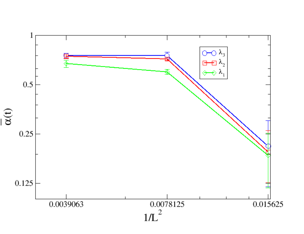
The particles form disconnected domains in the active model B, where the activity is constant or uniform. Despite an increase in activity, the length scale for the active model remains ideal ncomms5351. The outcomes are different for this model of inhomogeneous activity. Particles are accumulating in the middle, and the accumulation is changing as the intensity of activity increases. In the case of intensity 1, as shown in Fig 3, we see a lower accumulation than in the case of intensity 3, as shown in Fig 5. The length scale changes with a change in intensity. We now estimate the kinetics of growing A-particle domain at the center of the box, for different intensities , , . We measure the growth of A-particle domains at the center of the box in the following manner. We first change the continuous density field to binary density if and if , then calculate the mean size of domains of A-particles in the center of the box. Mean is calculated over independent realizations. As time progresses the domain size increases at the middle of the box. We estimate the length of the growing domains at the center of the box and plot the scaled length vs.time for three different intensities. In Fig. 6, the plot is shown for the three cases. Very clearly growth is faster for larger intensities and saturates at late times. The grows with time as, . We calculate the dynamic exponent . The plot of vs time is shown in Fig., 6(b). For all intensities up to some intermediate time remains between to and then decay to zero in the steady state. We find steady state is achieved faster for higher intensity. For comparison, we also calculate the characteristic length for pure passive model B and active model B with constant in Fig., 6(c). A straight line with slope is shown for the comparison of growing length for the two cases. We also plot the mean value of exponent for three different system sizes and in Fig. 6(d). The mean is obtained from the value of before it reaches the steady state (approaches zero). Which is very different from the asymptotic steady state as found in kinetics of other model systems new_1; new_2. Here due to finite system steady state is always a flat domain with saturated length and . Clearly the mean of the for growing domain before it reaches the steady state approaches value close to for large system sizes. Hence, the growth of accumulation of density in middle of the box for IAMB is much faster than that for the model B and active model B. Detail study of effect of activity on the growing domains in the active model in studied elsewere sudeep.
V Discussion
We have studied the steady state and dynamics of phase separation of active-particles: which experience the inhomogeneous activity on a two-dimensional
substrate. Activity parameter is distributed as Bivariate-Gaussian distribution at the center of the system, with a standard deviation of *(size of the system).
Unlike model a with constant activity parameters we have observed that accumulation of particles with variable densities are formed.
The accumulation increases by increasing the intensity of distribution. In the region outside the distribution or away from
the distribution, density phase separation is the same as for passive model B. chc2; chc; chc3
We also estimated the growth of A-particle domains in the center of the box with time. The domain of A-particle in the region of high activity grows as
a power law with time.
Hence our study gives an interesting steady state of density phase separation of active particles on a inhomogeneous patterned substrate and it can be useful to understand the trapping and transport of active particles in inhomogeneous systems. A detailed understanding of density phase separation is required to understand the mechanism of density phase separation in the inhomogeneous system.
VI References
References
- (1) J. T. Bonner, Proc. Natl. Acad. Sci. U.S.A. 95, 9355 (1998).
- (2) J. K. Parrish and W. M. Hammer (eds), Animal Group in Three Dimensions (Cambridge: Cambridge University Press) (1997).
- (3) D. Chen , Y. Wang, G. Wu, M. Kang, Y. Sun, and W. Yu, Chaos29, 113118 (2019).
- (4) M. C. Marchetti, J. F. Joanny, S. Ramaswamy, T. B. Liverpool, J. Prost, Madan Rao, and R. Aditi Simha Rev. Mod. Phys. 85, 1143 (2013).
- (5) H. H. Wensink, J. Dunkel, S. Heidenreich, K. Drescher, R. E. Goldstein, H. Lowen, and J.M Yeomans, Proc. Natl. Acad. Sci. U.S.A. , 109(36), 14313 (2012).
- (6) C. Dombrowski, Cisneros, S. Chatkaew, R. E. Goldstein, J. O. Kessler, Phys. Rev. Lett. 93, 098103 (2004).
- (7) A. Sokolov, I. S. Aranson, J. O. Kessler, R. E. Goldstein, Phys. Rev. Lett. 98, 158102 (2007).
- (8) L. H. Cisneros, R. Cortez, C. Dombrowski, R. E. Goldstein, J. E. Kessler, Exp. Fluids 43, 753 (2007).
- (9) C. W. Wolgemuth, Biophys J 95, 1574 (2008).
- (10) M. E. Cates, Rep. Prog. Phys. 75, 042601 (2012).
- (11) Jonathan R. Howse, Richard A. L. Jones, Anthony J. Ryan, Tim Gough, Reza Vafabakhsh, and Ramin Golestanian, Phys. Rev. Lett. 99, 048102 (2007)
- (12) S. J. Ebbens and J. R. Howse, Soft Matter 6, 738 (2010).
- (13) S. Thutupalli, R. Seemann and S. Herminghaus, New J. Phys. 13, 073021 (2011).
- (14) G. Volpe, I. Buttinoni, D. Vogt, H. Kümmerer and C. Bechinger, Soft Matter 7, 8815 (2011).
- (15) J. Palacci, S. Sacanna, A. P. Steinberg, D. J. Pine and P. M. Chaikin, Science 339, 940 (2013).
- (16) Ken A Hawick, Daniel P Playne. Modelling and Visualizing the Cahn-Hilliard-Cook Equation, Technical Report CSTN-049, 155 (2008).
- (17) J. W. Cahn and J. E Hilliard. Chem. Phys. 28, 267 (1958).
- (18) J. W. Cahn and J. E. Hilliard J. Chem. Phys. 31, 688 (1959).
- (19) R. Wittkowski, A. Tiribocchi, J. Stenhammar, R. J. Allen, D. Marenduzzo, and M. E. Cates, Nat. Comm. 5, 4351 (2014).
- (20) S. Pattanayak, R. Das, M. Kumar, and Shradha Mishra, Eur. Phys. J. E 42, 62 (2019).
- (21) P. Malgaretti and H. Stark, J. Chem. Phys. 146, 174901 (2017).
- (22) Bao-quan Ai, Qiu-yan Chen, Ya-feng He, Feng-guo Li, and Wei-rong Zhong Phys. Rev. E 88, 062129 (2013).
- (23) P. Dolai, A. Simha, and S. Mishra, Soft Matter, 14(29), 6145 (2018).
- (24) S. Ramaswamy, Annual Review of Condensed Matter Physics, 1323 (2010).
- (25) J. P. Singh and S. Mishra, Physica A: Statistical Mechanics and its Applications 544, 123530, (2020).
- (26) Y. Fily and M. C. Marchetti, Phys. Rev. Lett. 108, 235702 (2012).
- (27) J. Stenhammar, A. Tiribocchi, R. J. Allen, D. Marenduzzo and M. E. Cates, Phys. Rev. Lett. 111, 145702 (2013).
- (28) Ivo Buttinoni, Julian Bialké, Felix Kümmel, Hartmut Löwen, Clemens Bechinger, and Thomas Speck, Phys. Rev. Lett. 110, 238301 (2013).
- (29) Quan-Xing Liu, Arjen Doelman, Vivi Rottschäfer, Monique de Jager, Peter M. J. Herman, Max Rietkerk, and Johan van de Koppel, Proc. Natl Acad. Sci. USA 110, 11910 (2013).
- (30) Sanjay Puri, Vinod Wadhawan. Kinetics of Phase Transitions, CRC Press (2009).
- (31) J. Tailleur and M. E. Cates, Phys. Rev. Lett. 100, 218103 (2008).
- (32) M. E. Cates and J. Tailleur, Europhys. Lett. 101, 20010 (2013).
- (33) R Das, S Mishra, S Puri, EPL 121 37002 (2018).
- (34) A. Fick, Annalen der Physik 170, 59 (1855).
- (35) A. Paul, T. Laurila, V. Vuorinen, S.V. Divinski. Fick’s Laws of Diffusion. In: Thermodynamics, Diffusion and the Kirkendall Effect in Solids. Springer, Cham (2014).
- (36) Paul M Chaikin, T. C. Lubensky, Principles of condensed matter physics, Cambridge University Press (1995).
- (37) N Balakrishnan, and Chin-Diew Lai. Continuous Bivariate Distributions, Springer-Verlag Press (2009).
- (38) Richard W. Hamming, Numerical Methods for Scientists and Engineers, Mc-Graw-Hill (1973).
- (39) S. Paul, A. Bera and S.K. Das, Soft Matter 17, 645 (2021).
- (40) S. K. Das et al. J. Phys.: Condens. Matter 32, 184005 (2020).
- (41) Sudipta Pattanayak, Shradha Mishra, Sanjay Puri, arXiv:2101.10626 (2021).