Two-Step Image Dehazing with Intra-domain and Inter-domain Adaptation
Abstract
Caused by the difference of data distributions, intra-domain gap and inter-domain gap are widely present in image processing tasks. In the field of image dehazing, certain previous works have paid attention to the inter-domain gap between the synthetic domain and the real domain. However, those methods only establish the connection from the source domain to the target domain without taking into account the large distribution shift within the target domain (intra-domain gap). In this work, we propose a Two-Step Dehazing Network (TSDN) with an intra-domain adaptation and a constrained inter-domain adaptation. First, we subdivide the distributions within the synthetic domain into subsets and mine the optimal subset (easy samples) by loss-based supervision. To alleviate the intra-domain gap of the synthetic domain, we propose an intra-domain adaptation to align distributions of other subsets to the optimal subset by adversarial learning. Finally, we conduct the constrained inter-domain adaptation from the real domain to the optimal subset of the synthetic domain, alleviating the domain shift between domains as well as the distribution shift within the real domain. Extensive experimental results demonstrate that our framework performs favorably against the state-of-the-art algorithms both on the synthetic datasets and the real datasets.
Index Terms:
Image dehazing, intra-domain adaption, inter-domain adaption.I Introduction
Haze, fog or smoke usually affects visibility and obscures key information of the images. To deal with this issue, image dehazing has been widely studied in recent years which aims to recover the clear images from their corresponding hazy images. The whole procedure can be formulated as
| (1) |
where denotes the hazy image and denotes the clear image, denotes a pixel position in the image, denotes the global atmospheric light and denotes the transmission map. In homogeneous situation, the transmission map can be represented as , where and is the atmosphere scattering parameter and the scene depth, respectively.


Obviously, image dehazing is an ill-posed problem. Thus, many researchers try to transform this problem into a well-posed problem by estimating atmospheric light intensity and transmission map via certain priors [2, 3, 4]. However, those methods are not robust and tend to fail in some scenes, especially when the color of the objects is similar to atmospheric light. More recently, to avoid hand-craft priors, other researchers apply convolutional neural network to directly predict atmospheric light intensity and transmission map from training data [5, 6, 7]. However, due to lack of intermediate supervision, the estimation of atmospheric light intensity and transmission map is inaccurate which leads to undesirable results. Therefore, certain follow-up works [8, 9, 10, 1] propose the end-to-end dehazing frameworks to circumvent the evaluation process of intermediate variables. Those methods utilize neural networks to learn a mapping from hazy images to clear images directly. However, fused information, including atmosphere information (, ) and depth information (), is tightly coupled throughout the whole framework, causing instability in convergence and optimization. In addition, those methods do not consider the large intra-domain gap, which further reduces the robustness under different haze distributions, as illustrated in Figure 1(b).
Although changes in haze distribution would cause changes in model performance, there are always certain easy samples, on which the model can achieve the best dehazing performance. Motivated by this phenomenon and existing deep learning methods including disentangled representation learning [11, 12, 13, 14, 15] and unsupervised domain adaptation (UDA) [16, 17, 18, 19, 20, 21], we propose an intra-domain adaptation and a constrained inter-domain adaptation in this work to address above issues.
In intra-domain adaptation step, we design a multi-to-one dehazing framework to decouple fused information, and mine anchor distribution (easy sample) by loss-based deeply supervision. Then, we apply GAN-based adaptation to align other distributions to anchor distribution. By implementing such an information decoupling and adaptation, the difficulty of training each sub-network is reduced, e.g., the subsequent reconstruction network only needs to recover clear images from the anchor distribution, which promotes better and faster convergence of the model. More importantly, haze distribution shift within the synthetic domain is alleviated and performance under different haze distributions is improved.
Aforementioned domain adaptation within the synthetic domain achieves haze distribution invariant framework, but the gap between the real domain and the synthetic domain still exists. Thus, we propose the inter-domain adaptation based on the intra-domain adaptation to improve the generalization of the model under different domains. Although previous work [22] has discussed the domain shift and developed a network to address it, the bridge they built from arbitrary real haze distributions to arbitrary synthetic haze distributions increases the difficulty of image dehazing when real haze distributions are aligned to hard samples of the synthetic domain. In our work, we only establish the connection from the real distributions to the anchor distributions in the synthetic domain (easy samples) instead. With this constraint, distributions of the real domain are aligned to the optimal subset of the synthetic domain, which alleviates the domain shift between domains along with the distribution shift in the real domain. In addition, this mechanism that imposing constraint on features is similar to normalization [23], making underlying optimization problem more stable and smooth.
For image dehazing on synthetic datasets and real datasets, our proposed two-step image dehazing network (TSDN) achieves state-of-the-art performance against previous algorithms. The contributions of this work are summarized as follows:
We divide synthetic domain into subsets and mine the optimal subset (easy samples) by losses. By applying our proposed intra-domain adaption and information decoupling, we alleviate the distribution shift and make the optimization more stable.
Based on intra-domain adaptation, we propose a constrained inter-domain adaptation between real domain and synthetic domain. By aligning real haze distributions to the optimal subset of synthetic haze distributions, we solve the domain shift between domains and the distribution shift within real domain.
We conduct extensive experiments and comprehensive ablation studies on the synthetic datasets and the real datasets which validates the effectiveness of our proposed method.
Our domain adaptation module can be integrated into existing dehazing frameworks for performance improvement.
II Related Works
II-A Image Dehazing
Previous image dehazing methods can be divided into prior based methods and learning based methods.
II-A1 Prior-based methods
Those methods recover clear images through statistics prior, e.g., the albedo of the scene in [24]. Recently, researchers have explored different priors for image dehazing [2, 3, 25, 4]. Specifically, based on the observation that clear images have higher contrast than hazy images, Tan et al. [2] enhance the visibility of hazy images by maximizing local contrast. He [3] proposes dark channel prior (DCP) that the intensity of pixels in haze-free patches is very low in at least one color channel to achieve image dehazing. Besides, based on a generic regularity that small image patches typically exhibit a one-dimensional distribution in the RGB color space, Fattal [25] proposes a color-lines approach to recover the scene transmission. Zhu et al. [4] propose color attenuation prior to recover the scene depth of the hazy image with a supervised learning method.
All above methods heavily rely on hypothetical priors. However, those priors tend to lose effectiveness in complex scene, leading to performance drop.
II-A2 Learning-based methods
Different from the above methods, learning-based methods use convolutional neural networks to recover clear images from hazy images directly [5, 26, 8, 9, 10, 22, 1]. Specifically, an end-to-end system for transmission estimation is proposed in [5]. Ren et al. [26] design a multi-scale neural network for learning transmission maps from hazy images in a coarse-to-fine manner. Qiu et al. [9] propose a pix2pix model with an enhancer block which reinforces the dehazing effect in both color and details. A multi-scale boosted decoder with dense feature fusion is proposed to restore clear images in [1]. However, those methods do not take into account the intra-domain gap, resulting in less robustness in the case of haze distribution shift.
II-B Domain Adaptation
The purpose of domain adaptation is to eliminate the distribution difference between labeled source domain and target domain. Recently, numerous domain adaptation approaches have been proposed, including aligning the source domain and target domain distributions, generating a mapping between two domains, or creating ensemble models [27]. The alignment based methods can be divided into pixel-level alignment [28, 29, 30, 31, 32] and feature-level alignment [33, 34, 35]. The feature-level alignment methods mostly try to produce feature maps with the same distribution from images with different distributions. And the pixel-level alignment methods usually learn a transformation in the pixel space from one domain to the other [28].
With the introduction of GAN [36], adversarial learning begins to be used in other computer vision tasks, e.g., image generation [37, 38, 39], image-to-image translation [30, 40, 41, 42], etc. Among them, adversarial-based unsupervised domain adaptation (UDA) utilizes adversarial learning to learn domain invariant features. This framework usually consists of a generator and a discriminator, where they play min-max games to obtain the distribution migration from the source domain to the target domain.
In image dehazing field, Shao et al. [22] propose a bidirectional translation network to bridge the domain gap. However, they only consider the inter-domain gap. In this work, we further minimize the intra-domain gap to achieve extra performance gains.
II-C Deeply Supervised Learning
The deeply supervised learning is proposed in [43]. They apply the classifier on the deep feature layers of the neural networks to promote better convergence. Also, they draw a conclusion that more discriminative features will improve the final performance of the classifier. Recently, the deeply supervised learning is widely used in image classification [44], semantic segmentation [45], human pose estimation [46].
In this work, we append auxiliary supervision branch on the feature layer. Unlike classification tasks which want to make features more discriminative, we want to make features of the same scene images less discriminative, i.e., eliminating haze distribution shift in feature space. Furthermore, our supervised learning is based on the dehazing loss so that we can ensure all features are aligned to the best one.
III Method
In this section, we introduce our overall method in section III-A, intra-domain adaptation in section III-B, constrained inter-domain adaptation in section III-C and loss functions in section III-D.
III-A Method Overview
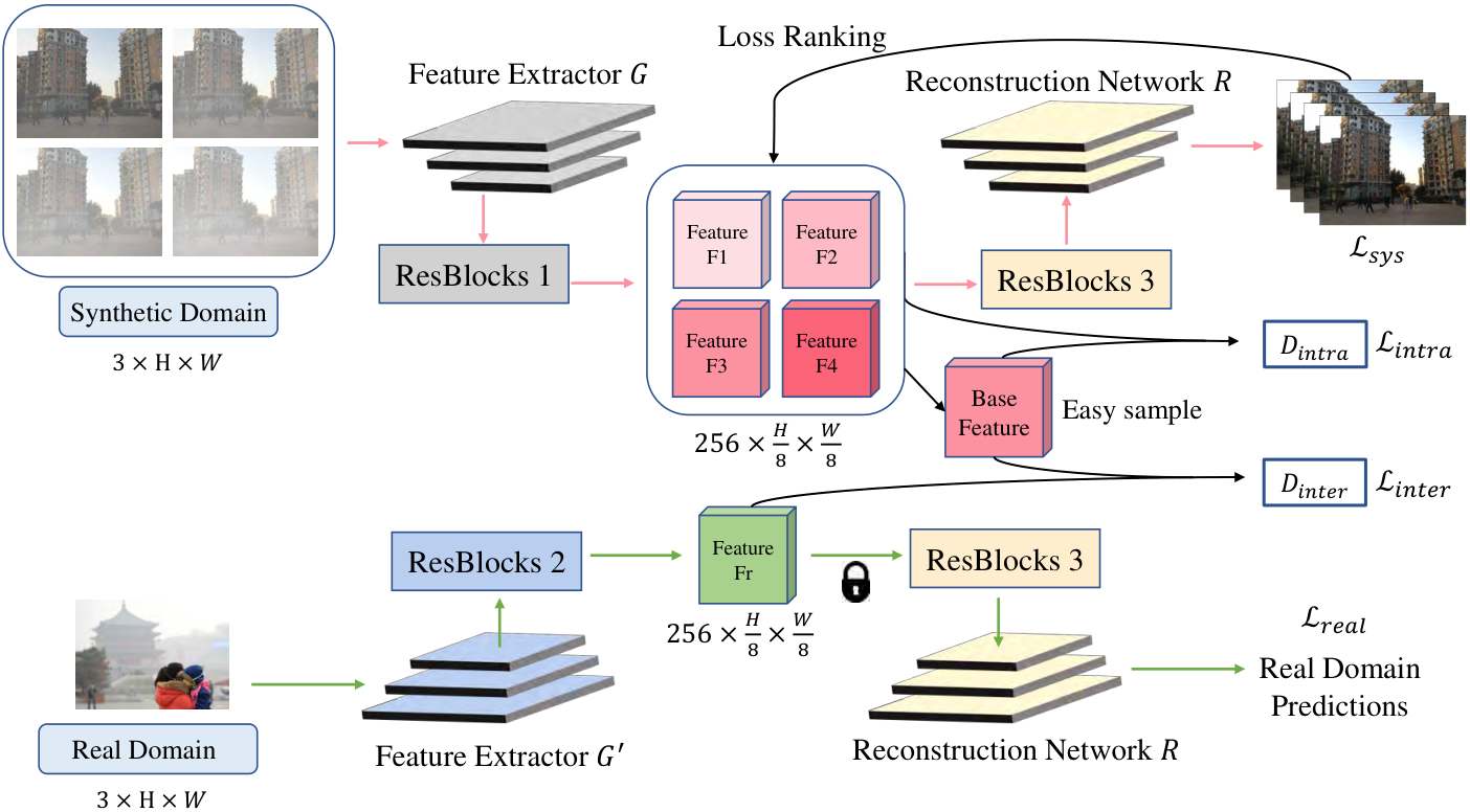
The overall framework of our work is illustrated in Figure 2. We design a multi-to-one dehazing framework to decouple fused information and mine easy samples. We append two auxiliary discriminators after feature extractor, guiding the network to learn distribution-invariant/domain-invariant fetaures based on those easy samples. Thus, all the features in the synthetic domain and the real domain would be aligned to the features of easy samples, which makes optimization more stable and performance more robust.
We first minimize the intra-domain gap then the inter-domain gap. In the intra-domain step, to reduce the effect of excessive differences in depth information, we take a set of hazy images in the same scene but with different haze distributions as input and get their corresponding features by the feature extractor . Then, we select base feature (easy sample) by comparing their dehazing losses and align all other features to the base feature by the intra-domain discriminator . Since those features possess the same depth information, this alignment is actually to decouple atmosphere information and from fused information and approximate them to the optimal and , where and serve as the anchor of different haze distributions. Thus, distribution shift can be alleviated in the feature space and subsequent module only need to learn how to reconstruct clear images from the easy sample, which accelerates convergence and improves performance. Finally, for the subsequent inter-domain adaptation, we mark easy samples in all scenes as the optimal subset of the synthetic domain.
In the inter-domain step, we begin by obtaining features of synthetic domain and real domain using feature extractor and , respectively. The hazy images of the synthetic domain are all selected from the optimal subset (marked in the intra-domain step), so the features of them are all base features (easy samples). Then, we perform the inter-domain adaptation from features of real domain to those base features using the inter-domain discriminator . By adding above constraints to the targets, we resolve the inter-domain gap along with intra-domain gap in the real domain.
III-B Intra-domain Adaptation
Generally, a clear image corresponds to multiple hazy images with different haze distributions. The goal of intra-domain adaptation is to align those hazy images and improve the performance on each image. To this end, we apply adversarial alignment in feature space via intra-domain discriminator .
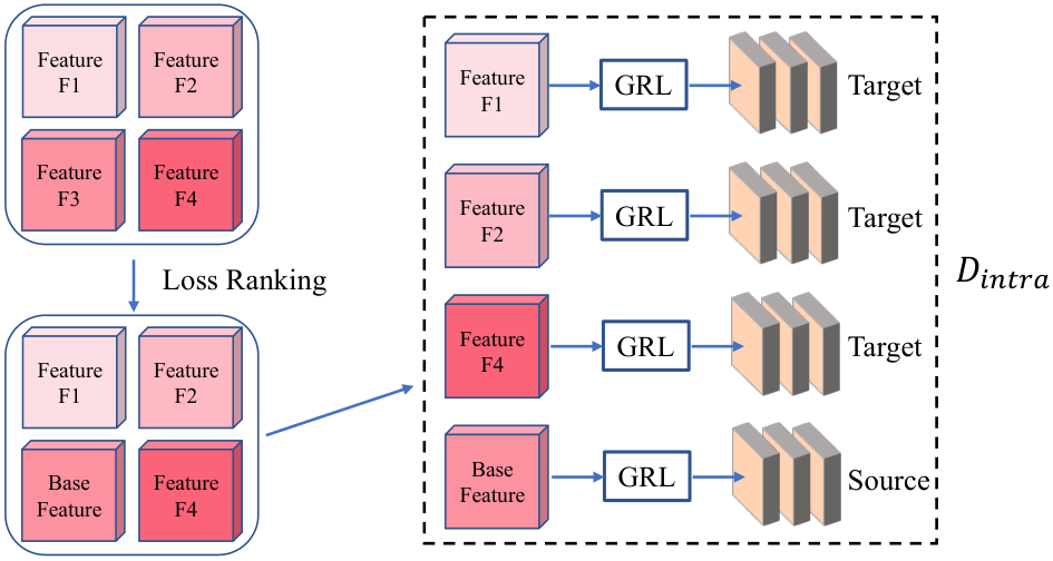
Suppose we have hazy images that belong to the same scene, we can extract features with a designed feature extractor network . To find the base feature to which all other features are aligned, we apply deeply supervised learning based on the dehazing losses. Specifically, we input all features into the reconstruction module to get their corresponding haze-free predictions and dehazing losses . According to those losses, we pick the feature with the lowest dehazing loss as base feature . Then, base feature along with other features are fed into a fully-convolutional network to generate intra-domain classification score maps. The score map has the same spatial resolution as the feature where each pixel position represents the intra-domain prediction of the same position in the feature. The loss function between the predicted classification score map and the label is binary cross-entropy loss which can be written as:
| (2) | ||||
where denotes a pixel position in the feature, denotes intra-domain label and denotes the total number of features we extracted. In our work, we set label of source and target as 1 and 0, respectively. Correspondingly, base feature is the intra-domain source and other features are the intra-domain target. For the discriminator , we optimize it using loss function Eq.(2). For feature extractor , we apply gradient reversal layer (GRL) [16] to perform adversarial learning. The pipeline of the deeply supervised learning and the intra-domain adaptation is illustrated in Figure 3. The discriminator tries to distinguish from () while feature extractor tries to generate similarly distributed and to confuse .
III-C Constrained Inter-domain Adaptation
The goal of the inter-domain adaptation is to close the inter-domain gap between the synthetic and real domains. We propose a constrained inter-domain adaptation which builds a bridge between real haze distributions and the optimal subset of the synthetic domain instead of the whole synthetic domain.
We perform the inter-domain adaptation in feature space by adversarial learning. Particularly, given a synthetic hazy image marked as an easy sample and a real hazy image , we extract their features and by extractor network and , respectively. Then, we obtain domain classification prediction maps of and by a fully-convolutional discriminator network . The prediction map has the same spatial shape as input and each position on it denotes domain label of the same position on input. We apply binary cross-entropy loss between the classification score map and the label, which can be written as:
| (3) | ||||
where denotes a pixel position in the feature and denotes inter-domain label. We set the synthetic domain as source and real domain as target, where source label is 1 and target label is 0. For feature extractor , we also apply gradient reversal layer (GRL) [16] to perform adversarial learning. In addition, we freeze reconstruction network at the beginning of the inter-domain adaptation during training to ensure that the real domain features fall into the optimal subset of the synthetic domain.
III-D Loss Functions
Given a synthetic dataset and a real dataset , where consists of a hazy subset and a clear subset while only contains a hazy set , We adopt following loss functions in our framework.
III-D1 Domain Adversarial Losses
III-D2 Image Dehazing Losses
Those losses measure the difference between the predicted images and the ground truth. In the synthetic domain, we apply loss to make sure the dehazed results are close to the clear images. Since a clear image corresponds to multiple hazy images, we further define the hazy subset as , where represents the -th hazy image corresponding to the -th clear image, denotes the total number of clear images and denotes the total number of hazy images. Thus, the predicted clear images can be defined as . The dehazing loss between and are defined as:
| (6) |
Besides, in order to improve the performance of our model in the real domain, we add the dark channel prior loss [3] and the total variation loss on the predicted real images [22]. We divide an image into patches and define the overall dark channel loss as:
| (7) |
where represents a patch and denotes the dark channel prior. The total variation loss is defined as:
| (8) | ||||
where and denote the horizontal position and the vertical position of an image, respectively. is the width of the image and is the height. So, the image dehazing loss in the real domain can be written as:
| (9) |
III-D3 Overall Loss
The overall loss is defined as weighted sum of all losses. In intra-domain training phase, the overall loss can be written as:
| (10) |
while in inter-domain training phase, the overall loss can be written as:
| (11) |
IV Experiments
We introduce related experiments and ablation studies in this section to verify our proposed method.
| DCP [3] | DehazeNet [5] | DCPDN [6] | EPDN [9] | GFN [49] | GDN [50] | DAdehazing [22] | MSBDN-DFF [1] | Ours | ||
|---|---|---|---|---|---|---|---|---|---|---|
| SOTS [47] | PSNR | 15.49 | 21.14 | 19.39 | 23.82 | 22.30 | 31.51 | 27.76 | 33.79 | 35.26 |
| SSIM | 0.646 | 0.853 | 0.659 | 0.893 | 0.886 | 0.982 | 0.928 | 0.983 | 0.985 | |
| HazeRD [48] | PSNR | 14.01 | 15.54 | 16.12 | 17.53 | 14.83 | 15.12 | 18.07 | 18.40 | 19.84 |
| SSIM | 0.390 | 0.432 | 0.407 | 0.593 | 0.802 | 0.833 | 0.632 | 0.881 | 0.892 |


IV-A Experimental details
IV-B Datasets
We choose RESIDE [47] dataset as our training dataset. For the intra-domain adaptation step, we randomly sample 8000 hazy images from ITS (Indoor Training Set) and 8000 hazy images from OTS (Outdoor Training Set). We utilize 4 same scene images with haze distribution shift to represent the varied haze distributions of the same scene and we explore 2000 indoor scenes and 2000 outdoor scenes to train our network. In other words, there are total 20,000 images (including clear labels) in the synthetic training set. For the inter-domain adaptation step, we randomly sample 3000 real hazy images from URHI (Unannotated Realistic Hazy Images). To achieve data augmentation, we randomly crop images to and randomly flip the cropped images horizontally during the training phase. Furthermore, we ensure that the crop areas and horizontal directions of the same scene images (four hazy images and one clear image) are consistent in each iteration.
IV-C Implementation details
We implement our method using PyTorch [51] framework, and we conduct experiments on both our designed base network (encoder-decoder architecture with residual blocks in Figure 2) and MSBDN-DFF [1] architecture. First, we train the dehazing module ( and ) and the intra-domain discriminator within the synthetic domain for 200 epochs. For the dehazing module, we apply the SGD [52] optimizer with learning rate , momentum and weight decay . For the intra-domain discriminator, we apply the Adam [53] optimizer with learning rate , and . We set parameter of reversed gradients as 0.1 in GRL module. Then, we adapt model to real hazy images by training network , and inter-domain discriminator for 20 epochs. Since all the features need to fall into the optimal subset of the synthetic domain, we freeze reconstruction network for 15 epoch and fine-tuned it for 5 epoch. We apply SGD optimizer with learning rate for the dehazing module and Adam optimizer with learning rate for the inter-domain discriminator.


IV-D Results on Synthetic Datasets
To evaluate the effectiveness of our proposed intra-domain adaptation, we train our model on SOTS [47] dataset and HazeRD [48] dataset and compare the results with other previous methods.
To verify the robustness in the case of distribution shifts, we test the dehazing performance of several models under different haze distributions, as shown in Figure 4. From those results, we can observe that previous algorithms all encounter the phenomenon of performance drop when facing different haze distributions, e.g., magnified area in the images. In other words, when the haze distribution is a hard sample, the dehazed image has higher chance that it remains haze in global or detail. Compared with previous methods, our approach generates clearer images under different haze situations which verifies the effectiveness of the intra-domain adaptation (more detailed proof can be found in IV-F).
The quantitative evaluation are shown in Table I. Our method achieves the best performance on both PSNR and SSIM. Compared with the state-of-the-art method MSBDN-DFF [1], our method achieves performance gain on both SOTS [47] and HazeRD [48].


IV-E Results on Real Images
To evaluate our proposed constrained inter-domain adaptation between the synthetic domain and the real domain, we conduct experiments on the real dataset RTTS [47] and compare visual results with other previous methods.
The visual results are shown in Figure 5. From the results, we can observe that previous dehazing methods have different limitations on real images. Specifically, DCP [3] suffers from serious color distortion and overexposure, e.g., the first, third and fourth rows of Figure 5 (b). Besides, the dehazed results of Dehazenet [5], FFA [10] and MSBDN-DFF [1] all have residual haze, e.g., the first, fourth and sixth rows of Figure 5 (c), (f) and (g). In addition, the dehazed results of EPDN [9] suffer from brightness issues (much darker), e.g., the third row and the traffic signs in the seventh row of Figure 5 (d) and color distortion (some results are more yellow than other methods), e.g., the sixth and seventh rows of Figure 5 (d). Furthermore, DAdehazing [22] reaches better visual results than the other previous methods since they integrate the inter-domain adaptation in their approach. The overall brightness and the color are well-maintained during dehazing process. However, there is still some residual haze, e.g., the trees in the fourth row of Figure 5 (e). In addition, some results of DAdehazing become less realistic or blur, e.g., the people in the first row, the trees in the fourth row and the people in the sixth row of Figure 5 (e). Those problems are caused by only considering the inter-domain gap between the source and the target without considering the intra-domain gap of the target. when the distribution of the real domain are aligned to the hard samples of the synthetic domain, the difficulty of image dehazing is increased. Overall, the method we proposed achieves the best performance in removing haze, maintaining the color and brightness of the images, and restoring details.
IV-F Ablation Study
In order to verify the effectiveness of each module in our proposed method, we conduct ablation studies on the intra-domain adaptation and the inter-domain adaptation.
In the intra-domain adaptation part, we conduct ablation study using the following settings: 1) BS: base network; 2) BS+ITA: base network with the intra-domain adaptation; 3) BS+ITA+LDS: base network with the intra-domain adaptation and the loss-based deep supervision.
| Network | ITA | LDS | PSNI | SSIM | |
|---|---|---|---|---|---|
| SOTS | Base | 23.80 | 0.881 | ||
| Base | ✓ | 27.32 | 0.929 | ||
| Base | ✓ | ✓ | 28.13 | 0.941 | |
| MSBDN-DFF | 33.79 | 0.983 | |||
| MSBDN-DFF | ✓ | 34.45 | 0.984 | ||
| MSBDN-DFF | ✓ | ✓ | 35.26 | 0.985 |
The quantitative results of the intra-domain adaptation are shown in Table II, which demonstrates that base network with the intra-domain adaptation and the loss-based deep supervision achieves the best performance. To further prove that the improvement on performance is promoted by the intra-domain adaptation, we compare the intra-domain gap under all three methods. Instead of directly measuring the distribution similarity of the features which is not intuitive, we utilize dehazing losses to measure the intra-domain gap. In other words, if the dehazing losses of the same scene are less discrete, the features of the same scene are more closely aligned. Specifically, we calculate the range, the standard deviation and the coefficient of variation of the dehazing losses in each scene and take the average of all scenes. The results are shown in Figure 6. From the results, we can observe that dehazing losses decrease faster after we apply the intra-domain adaptation to base network. Moreover, dehazing losses are more compact in methods with the intra-domain adaptation which demonstrates that the features of the same scene images are aligned in feature space.
In the inter-domain part, we conduct ablation study with the following settings: 1) BS: base network; 2) BS+ITE: base network with the inter-domain adaptation; 3) BS+ITA: base network with the intra-domain adaptation; 4) BS+ITA+ITE: base network with the intra-domain and the inter-domain adaptation.
The visual results are shown in Figure 7. The result of base network has residual haze due to the domain gap. This phenomenon is alleviated by the intra-domain adaptation or the inter-domain adaptation. However, color distortion appears if the inter-domain adaptation is directly applied because the network is sensitive to the haze distribution of the input image. Base network with intra-domain adaptation and inter-domain adaptation achieve the best performance.
V Conclusion
In this paper, we propose a two-step dehazing network (TSDN) which consists of an intra-domain adaptation step and a constrained inter-domain adaptation step. First, we subdivide the distributions within the synthetic domain into subsets and mine the optimal subset (easy samples) by loss-based supervision. Then, we propose the intra-domain adaptation within the synthetic domain to alleviate the distribution shift. Specifically, we align features with different haze distributions to base feature (easy sample) by adversarial learning. Finally, we conduct the constrained inter-domain adaptation from the real domain to the optimal subset of the synthetic domain, alleviating the domain shift between domains as well as the distribution shift within the real domain. Moreover, when the distribution is aligned to the easy sample, the difficulty of image dehazing is reduced, which enhances the performance. Extensive experimental results demonstrate that our method performs favorably against the state-of-the-art algorithms both on the synthetic datasets and the real datasets.
References
- [1] H. Dong, J. Pan, L. Xiang, Z. Hu, X. Zhang, F. Wang, and M.-H. Yang, “Multi-scale boosted dehazing network with dense feature fusion,” in Proceedings of the IEEE/CVF Conference on Computer Vision and Pattern Recognition, 2020, pp. 2157–2167.
- [2] R. T. Tan, “Visibility in bad weather from a single image,” in 2008 IEEE Conference on Computer Vision and Pattern Recognition. IEEE, 2008, pp. 1–8.
- [3] K. He, J. Sun, and X. Tang, “Single image haze removal using dark channel prior,” IEEE transactions on pattern analysis and machine intelligence, vol. 33, no. 12, pp. 2341–2353, 2010.
- [4] Q. Zhu, J. Mai, and L. Shao, “A fast single image haze removal algorithm using color attenuation prior,” IEEE transactions on image processing, vol. 24, no. 11, pp. 3522–3533, 2015.
- [5] B. Cai, X. Xu, K. Jia, C. Qing, and D. Tao, “Dehazenet: An end-to-end system for single image haze removal,” IEEE Transactions on Image Processing, vol. 25, no. 11, pp. 5187–5198, 2016.
- [6] H. Zhang and V. M. Patel, “Densely connected pyramid dehazing network,” in Proceedings of the IEEE conference on computer vision and pattern recognition, 2018, pp. 3194–3203.
- [7] H. Zhang, V. Sindagi, and V. M. Patel, “Joint transmission map estimation and dehazing using deep networks,” IEEE Transactions on Circuits and Systems for Video Technology, vol. 30, no. 7, pp. 1975–1986, 2019.
- [8] R. Li, J. Pan, Z. Li, and J. Tang, “Single image dehazing via conditional generative adversarial network,” in Proceedings of the IEEE Conference on Computer Vision and Pattern Recognition, 2018, pp. 8202–8211.
- [9] Y. Qu, Y. Chen, J. Huang, and Y. Xie, “Enhanced pix2pix dehazing network,” in Proceedings of the IEEE Conference on Computer Vision and Pattern Recognition, 2019, pp. 8160–8168.
- [10] X. Qin, Z. Wang, Y. Bai, X. Xie, and H. Jia, “Ffa-net: Feature fusion attention network for single image dehazing.” in AAAI, 2020, pp. 11 908–11 915.
- [11] X. Chen, Y. Duan, R. Houthooft, J. Schulman, I. Sutskever, and P. Abbeel, “Infogan: Interpretable representation learning by information maximizing generative adversarial nets,” arXiv preprint arXiv:1606.03657, 2016.
- [12] I. Higgins, L. Matthey, A. Pal, C. Burgess, X. Glorot, M. Botvinick, S. Mohamed, and A. Lerchner, “beta-vae: Learning basic visual concepts with a constrained variational framework,” 2016.
- [13] L. Tran, X. Yin, and X. Liu, “Disentangled representation learning gan for pose-invariant face recognition,” in Proceedings of the IEEE conference on computer vision and pattern recognition, 2017, pp. 1415–1424.
- [14] Z. Zhang, L. Tran, X. Yin, Y. Atoum, X. Liu, J. Wan, and N. Wang, “Gait recognition via disentangled representation learning,” in Proceedings of the IEEE/CVF Conference on Computer Vision and Pattern Recognition, 2019, pp. 4710–4719.
- [15] G. Wang, H. Han, S. Shan, and X. Chen, “Cross-domain face presentation attack detection via multi-domain disentangled representation learning,” in Proceedings of the IEEE/CVF Conference on Computer Vision and Pattern Recognition, 2020, pp. 6678–6687.
- [16] Y. Ganin and V. Lempitsky, “Unsupervised domain adaptation by backpropagation,” in International conference on machine learning. PMLR, 2015, pp. 1180–1189.
- [17] M. Long, H. Zhu, J. Wang, and M. I. Jordan, “Unsupervised domain adaptation with residual transfer networks,” arXiv preprint arXiv:1602.04433, 2016.
- [18] K. Saito, K. Watanabe, Y. Ushiku, and T. Harada, “Maximum classifier discrepancy for unsupervised domain adaptation,” in Proceedings of the IEEE conference on computer vision and pattern recognition, 2018, pp. 3723–3732.
- [19] G. Kang, L. Jiang, Y. Yang, and A. G. Hauptmann, “Contrastive adaptation network for unsupervised domain adaptation,” in Proceedings of the IEEE/CVF Conference on Computer Vision and Pattern Recognition, 2019, pp. 4893–4902.
- [20] W.-G. Chang, T. You, S. Seo, S. Kwak, and B. Han, “Domain-specific batch normalization for unsupervised domain adaptation,” in Proceedings of the IEEE/CVF Conference on Computer Vision and Pattern Recognition, 2019, pp. 7354–7362.
- [21] H. Tang, K. Chen, and K. Jia, “Unsupervised domain adaptation via structurally regularized deep clustering,” in Proceedings of the IEEE/CVF conference on computer vision and pattern recognition, 2020, pp. 8725–8735.
- [22] Y. Shao, L. Li, W. Ren, C. Gao, and N. Sang, “Domain adaptation for image dehazing,” in Proceedings of the IEEE/CVF Conference on Computer Vision and Pattern Recognition, 2020, pp. 2808–2817.
- [23] S. Ioffe and C. Szegedy, “Batch normalization: Accelerating deep network training by reducing internal covariate shift,” in International conference on machine learning. PMLR, 2015, pp. 448–456.
- [24] R. Fattal, “Single image dehazing,” ACM transactions on graphics (TOG), vol. 27, no. 3, pp. 1–9, 2008.
- [25] ——, “Dehazing using color-lines,” ACM transactions on graphics (TOG), vol. 34, no. 1, pp. 1–14, 2014.
- [26] W. Ren, S. Liu, H. Zhang, J. Pan, X. Cao, and M.-H. Yang, “Single image dehazing via multi-scale convolutional neural networks,” in European conference on computer vision. Springer, 2016, pp. 154–169.
- [27] G. Wilson and D. J. Cook, “A survey of unsupervised deep domain adaptation,” ACM Transactions on Intelligent Systems and Technology (TIST), vol. 11, no. 5, pp. 1–46, 2020.
- [28] K. Bousmalis, N. Silberman, D. Dohan, D. Erhan, and D. Krishnan, “Unsupervised pixel-level domain adaptation with generative adversarial networks,” in Proceedings of the IEEE conference on computer vision and pattern recognition, 2017, pp. 3722–3731.
- [29] A. Shrivastava, T. Pfister, O. Tuzel, J. Susskind, W. Wang, and R. Webb, “Learning from simulated and unsupervised images through adversarial training,” in Proceedings of the IEEE conference on computer vision and pattern recognition, 2017, pp. 2107–2116.
- [30] J.-Y. Zhu, T. Park, P. Isola, and A. A. Efros, “Unpaired image-to-image translation using cycle-consistent adversarial networks,” in Proceedings of the IEEE international conference on computer vision, 2017, pp. 2223–2232.
- [31] T. Kim, M. Cha, H. Kim, J. K. Lee, and J. Kim, “Learning to discover cross-domain relations with generative adversarial networks,” arXiv preprint arXiv:1703.05192, 2017.
- [32] Z. Yi, H. Zhang, P. Tan, and M. Gong, “Dualgan: Unsupervised dual learning for image-to-image translation,” in Proceedings of the IEEE international conference on computer vision, 2017, pp. 2849–2857.
- [33] C. Chen, W. Xie, W. Huang, Y. Rong, X. Ding, Y. Huang, T. Xu, and J. Huang, “Progressive feature alignment for unsupervised domain adaptation,” in Proceedings of the IEEE Conference on Computer Vision and Pattern Recognition, 2019, pp. 627–636.
- [34] B. Sun and K. Saenko, “Deep coral: Correlation alignment for deep domain adaptation,” in European conference on computer vision. Springer, 2016, pp. 443–450.
- [35] E. Tzeng, J. Hoffman, K. Saenko, and T. Darrell, “Adversarial discriminative domain adaptation,” in Proceedings of the IEEE conference on computer vision and pattern recognition, 2017, pp. 7167–7176.
- [36] I. Goodfellow, J. Pouget-Abadie, M. Mirza, B. Xu, D. Warde-Farley, S. Ozair, A. Courville, and Y. Bengio, “Generative adversarial nets,” in Advances in neural information processing systems, 2014, pp. 2672–2680.
- [37] J. Bao, D. Chen, F. Wen, H. Li, and G. Hua, “Cvae-gan: Fine-grained image generation through asymmetric training,” in Proceedings of the IEEE International Conference on Computer Vision (ICCV), Oct 2017.
- [38] J. Yang, A. Kannan, D. Batra, and D. Parikh, “Lr-gan: Layered recursive generative adversarial networks for image generation,” arXiv preprint arXiv:1703.01560, 2017.
- [39] C. H. Lin, C.-C. Chang, Y.-S. Chen, D.-C. Juan, W. Wei, and H.-T. Chen, “Coco-gan: generation by parts via conditional coordinating,” in Proceedings of the IEEE International Conference on Computer Vision, 2019, pp. 4512–4521.
- [40] Y. Choi, M. Choi, M. Kim, J.-W. Ha, S. Kim, and J. Choo, “Stargan: Unified generative adversarial networks for multi-domain image-to-image translation,” in Proceedings of the IEEE conference on computer vision and pattern recognition, 2018, pp. 8789–8797.
- [41] P. Isola, J.-Y. Zhu, T. Zhou, and A. A. Efros, “Image-to-image translation with conditional adversarial networks,” in Proceedings of the IEEE conference on computer vision and pattern recognition, 2017, pp. 1125–1134.
- [42] T.-C. Wang, M.-Y. Liu, J.-Y. Zhu, A. Tao, J. Kautz, and B. Catanzaro, “High-resolution image synthesis and semantic manipulation with conditional gans,” in Proceedings of the IEEE conference on computer vision and pattern recognition, 2018, pp. 8798–8807.
- [43] C.-Y. Lee, S. Xie, P. Gallagher, Z. Zhang, and Z. Tu, “Deeply-supervised nets,” in Artificial intelligence and statistics, 2015, pp. 562–570.
- [44] D. Sun, A. Yao, A. Zhou, and H. Zhao, “Deeply-supervised knowledge synergy,” in Proceedings of the IEEE Conference on Computer Vision and Pattern Recognition, 2019, pp. 6997–7006.
- [45] Z. Zhang, X. Zhang, C. Peng, X. Xue, and J. Sun, “Exfuse: Enhancing feature fusion for semantic segmentation,” in Proceedings of the European Conference on Computer Vision (ECCV), 2018, pp. 269–284.
- [46] A. Newell, K. Yang, and J. Deng, “Stacked hourglass networks for human pose estimation,” in European conference on computer vision. Springer, 2016, pp. 483–499.
- [47] B. Li, W. Ren, D. Fu, D. Tao, D. Feng, W. Zeng, and Z. Wang, “Benchmarking single-image dehazing and beyond,” IEEE Transactions on Image Processing, vol. 28, no. 1, pp. 492–505, 2019.
- [48] Y. Zhang, L. Ding, and G. Sharma, “Hazerd: an outdoor scene dataset and benchmark for single image dehazing,” in 2017 IEEE international conference on image processing (ICIP). IEEE, 2017, pp. 3205–3209.
- [49] W. Ren, L. Ma, J. Zhang, J. Pan, X. Cao, W. Liu, and M.-H. Yang, “Gated fusion network for single image dehazing,” in Proceedings of the IEEE Conference on Computer Vision and Pattern Recognition, 2018, pp. 3253–3261.
- [50] X. Liu, Y. Ma, Z. Shi, and J. Chen, “Griddehazenet: Attention-based multi-scale network for image dehazing,” in Proceedings of the IEEE International Conference on Computer Vision, 2019, pp. 7314–7323.
- [51] A. Paszke, S. Gross, S. Chintala, G. Chanan, E. Yang, Z. DeVito, Z. Lin, A. Desmaison, L. Antiga, and A. Lerer, “Automatic differentiation in pytorch,” 2017.
- [52] L. Bottou, “Large-scale machine learning with stochastic gradient descent,” in Proceedings of COMPSTAT’2010. Springer, 2010, pp. 177–186.
- [53] D. P. Kingma and J. Ba, “Adam: A method for stochastic optimization,” arXiv preprint arXiv:1412.6980, 2014.