Wasserstein Graph Neural Networks for
Graphs with Missing Attributes
Abstract.
Missing node attributes is a common problem in real-world graphs. Graph neural networks have been demonstrated power in graph representation learning while their performance is affected by the completeness of graph information. Most of them are not specified for missing-attribute graphs and fail to leverage incomplete attribute information effectively. In this paper, we propose an innovative node representation learning framework, Wasserstein Graph Neural Network (WGNN), to mitigate the problem. To make the most of limited observed attribute information and capture the uncertainty caused by missing values, we express nodes as low-dimensional distributions derived from the decomposition of the attribute matrix. Furthermore, we strengthen the expressiveness of representations by developing a novel message passing schema that aggregates distributional information from neighbors in the Wasserstein space. We test WGNN in node classification tasks under two missing-attribute cases on both synthetic and real-world datasets. In addition, we find WGNN suitable to recover missing values and adapt them to tackle matrix completion problems with graphs of users and items. Experimental results on both tasks demonstrate the superiority of our method.
Keywords:
Graph representation, Message passing, Missing-attribute graph, Node classification, Matrix completion.1. Introduction
Graphs are ubiquitous data structures, where nodes usually have associated attributes. There have been many impressive and practical machine learning methods on graphs, particularly, graph representation learning (Perozzi et al. 2014; Grover and Leskovec 2016; Gilmer et al. 2017) which attempts to embed local structural and attribute information into node representations. Graph representation learning methods underlay various downstream graph-based learning tasks such as node classification and link prediction while the accuracy of most applications is affected by the completeness of graph data. Unfortunately, missing attributes are common in many real-world graph data. For instance, in social networks such as Facebook and Twitter, users tend to hide or selectively publish their personal information for privacy concerns. In molecular networks like protein-protein association networks (Szklarczyk et al. 2019), where nodes represent proteins and edges indicate biological associations, it is difficult to obtain complete information about the sequences and molecular structures of newly discovered proteins. In general, we can categorize node attribute missing issues into two cases: 1). Entirely missing: missing entire attributes on some nodes, 2). Partially missing: missing partial attributes on all nodes. In this paper, we investigate graph learning on graphs with missing-attribute.
Existing graph representation learning methods are not specified for missing-attribute graphs. Random-walk based network embedding approaches (Perozzi et al. 2014; Grover and Leskovec 2016) exploit graph structure information to preserve pre-specified node similarities in the embedding space without considering informative node attributes. Message-passing (Gilmer et al. 2017) based graph neural networks (GNNs) incorporate node attributes and graph structure effectively by aggregating information from neighborhoods. However, to handle incomplete node attributes, they usually need to leverage matrix imputation techniques (Troyanskaya et al. 2001; Hastie et al. 2015) for missing values estimation before learning. Despite missing value imputation (MVI) being a well-studied problem in data mining and analysis, it is still a big challenge to recover missing values with inadequate observed information (Dong and Peng 2013; Lin and Tsai 2020). Moreover, imputation methods might introduce noise in representations and restrict graph embedding approaches to model uncertainty caused by missing attributes.
In this paper, we propose a significant assumption on data: attributes of each node are sampled from low-dimensional mixture distributions, similar to the low-rank assumption in most matrix imputation algorithms. More precisely, we assume that there are some latent factors of nodes and each node has a distribution over these latent factors, called node-factor distribution. Meanwhile, each latent factor has a distribution over node attributes, called factor-attribute distribution. For instance, in text mining where nodes represent documents with words as their attributes, topics are their latent factors (Arora et al. 2012). In practice, the number of (principal) latent factors is usually small. Following this assumption, we employ a matrix-factorization-based method to obtain latent factors from observed node attributes. Thereby, we can also get the node-factor distributions of each node which are exactly low-dimensional node distributional representations. In this way, we can capture the uncertainty caused by incomplete attribute information.
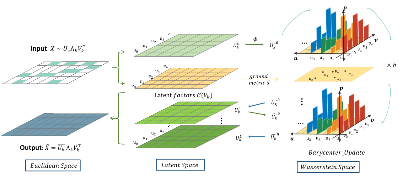
To handle various graph learning tasks on missing-attribute graphs, we develop an ingenious graph embedding framework, Wasserstein Graph Neural Network (WGNN), which can generate powerful node representations. Although the aforementioned node distributional representations incorporate attribute and uncertainty information, they fail to reflect graph structure information which is essential for graph learning. Inspired by message-passing based GNNs, we adapt the neighborhood aggregation process in GNNs to the node distributional representations. The key idea is to generalize aggregator function to Wasserstein space (Frogner et al. 2019) by computing the Wasserstein Barycenters - the mean of distribution of neighbors for node distributional representation update. In addition, we can pull node distributions back to the original Euclidean space and generate new Euclidean embeddings. Figure 1 depicts the general architecture. WGNN combines the propagation process with a multi-layer perceptron layer (MLP).
To comprehensively investigate the representation ability of WGNN, we design a SVD-based WGNN variant for node classification concerning two missing-attribute cases: partially missing and entirely missing. We validate the strengths of our proposed framework on both synthetic and real-world graphs. Extensive empirical results show that compared with all baselines, greatly boosts the performance. Furthermore, although our framework is not originally designed for missing values prediction, it can be naturally adapted for the matrix completion task with additional reconstruction constraints. Compared with SOTA matrix completion algorithms (Rao et al. 2015; Monti et al. 2017; Hartford et al. 2018; Zhang and Chen 2020), our method relies on much fewer parameters and has competitive performance.
Contributions. Overall, our contribution can be summarized as follows: 1. We propose a novel missing-attribute graph learning framework in Wasserstein space, called WGNN, to elegantly generate powerful node representations without explicit data imputation. Our performance is far surpassing that of baselines; 2. We extend WGNN on multi-graph and adapt it for matrix completion with the content of users and items and achieve comparable results of SOTA algorithms with much fewer parameters.
2. Background and Related Work
Graph representation learning. In this paper, we focus on learning node representations on attributed graphs. There are many effective graph embedding approaches, such as DeepWalk (Bojchevski and Günnemann 2018), node2vec (Grover and Leskovec 2016), GenVetor (Duarte et al. 2019), which embed nodes into a lower-dimension Euclidean space and preserve graph structure while most of them disregard node informative attributes. The advent of graph neural networks (Bruna et al. 2014; Kipf and Welling 2017; Hamilton et al. 2017; Veličković et al. 2017; Gilmer et al. 2017; Klicpera et al. 2019) fills the gap, by defining graph convolutional operations in spectral domain or aggregator functions in spatial domain. Although they achieved great success, they highly rely on the completeness and adequacy of attribute information.
Machine learning with missing data. To handle missing data, most machine learning methods rely on data imputation. There is a variety of missing value imputation (MVI) techniques such as mean-filling, KNN imputation (Troyanskaya et al. 2001), softimpute (Hastie et al. 2015) with SVD, multivariate imputation (Van Buuren 2007; Buuren and Groothuis-Oudshoorn 2010). Also, many deep learning methods are proposed to perform the imputation tasks (Gondara and Wang 2017; Yoon et al. 2018; Spinelli et al. 2020). One work worth noting is Muzellec et al (Muzellec et al. 2020), which also uses optimal transport to solve the data missing problem. However, it only targets on imputation on general data (without structures) instead of graphs and has a very different methodology. The "imputing before learning" strategy has an important limitation: the performance of models is inherently constrained by the reconstruction ability of the used imputation methods. However, these imputation methods would not always work especially in the extreme missing cases.
Recently, some advanced models have been developed to directly handle missing data targeting at specified tasks. GRAPE (You et al. 2020) tackles missing data problems for label prediction and feature imputation. Unlike our work, the missing data is not originally on the graph nodes, but GRAPE represents their two tasks as graph-based problems by leveraging a created bipartite graph. Another recent work, SAT (Chen et al. 2020), models link prediction and node attribute imputation on missing-attribute graphs with shared-latent space assumption. Different from these works, our WGNN is a graph representation learning framework that focuses on learning node representations with incomplete attribute matrix as input without imputation; and it can be adapted to various downstream graph-based tasks.
3. Wasserstein Graph Neural Network (WGNN)
In this paper, we propose a graph embedding framework, named Wasserstein Graph Neural Network (WGNN) specified for missing-attribute graphs. WGNN (depicted in Figure 1) consists of three main components: distributional representation generation to encode observed attribute and uncertainty information, Wasserstein aggregation process to update node distributional representations involving graph structure in a low-dimensional Wasserstein space, and Euclidean representation generation to pull nodes back to a high-dimensional Euclidean space for downstream tasks.
3.1. Preliminary
3.1.1. Notations
For a matrix , we write , where is the -th row of . We denote as the set of rows of and as the set of columns of . Give a missing-attribute graph with a collection of node attributes , we denote observed attribute matrix as its incomplete node attribute matrix, whose missing values are filled with zeros, and is the attribute vector/Euclidean embedding of the -th node.
3.1.2. Assumption
We assume that observed values of come from a collection of latent factor vectors where and each node (e.g. node ) may contain attributes from several latent distributions in particular proportions (). Given , we assume that there exists low-rank matrices and such that is the embedding of latent factors and is the weight/probability vectors of nodes affected by latent factors.
3.1.3. Wasserstein Distance and Wasserstein Barycenter
- •
Wasserstein distance is an optimal transport metric which measures the distance traveled in transporting the mass in one distribution to match another. The -Wasserstein distance between two distributions and over a metric space is defined as
where is the the set of probabilistic couplings on , is a ground metric on . In this paper, we take . The Wasserstein space is a metric space that endows probability distributions with the Wasserstein distance.
- •
Wasserstein barycenter of distributions over is an optimizer to the problem:
where denotes the set of all probability measures on . If are discrete distributions supported by , support points of barycenter must contain all possible combinations of , i.e.:
(1)
3.2. Distributional representation generation
According to the proposed assumption, nodes are mixtures of latent factors and can be expressed as low-dimensional node-factor distributions. In this section, we develop an effective method with matrix decomposition (in our implementation, we use SVD) on the observed attribute matrix to construct a collection of principal latent factors. Thereby, we obtain latent factor embeddings and low-dimensional distributional representations . The low-rank assumption, which is prevalent in matrix completion, allows missing value imputation methods to obtain a dense and low-rank matrix through dimension reduction techniques. In light of this, we employ SVD to the incomplete attribute matrix (similar to LSI(Dumais 2004)). Precisely, through compact SVD, we have , where is so-called the principal component matrix, is a square diagonal matrix with ( are singular values of in descending order) and is the basis matrix. Here, we indicate that is a collection of latent factors. For given , considering the first principal latent factors, we denote , and write
| (2) |
We say is the weight matrix with respect to latent factors with as the embedding matrix. Allowing negative probability, can be regarded as a generalized discrete distribution supported by . Then we formulate a general transformation function to embed to a standard discrete probability space:
| (3) |
where is the distributional representation matrix and is a reversible non-negative function depending on data. In our implementation, so that .
3.3. The Wasserstein aggregation process
Through the transformation , we obtain discrete node-factor distributions which incorporate valid observed attribute information and uncertainty of missing attributes. Noting that Euclidean embeddings fail to express the semantic information of distributions, stemming from the limited expressive capacity of Euclidean space, we take Wasserstein space as the embedding space. Similar to many graph learning methods, we attempt to reflect graph structures in node representations by aggregating information from neighbors.
We first formulate the Wasserstein distance. Denote as the set of support points of , here we define a ground metric over and obtain the distance matrix as follows:
| (4) |
Then we have the corresponding Wasserstein metric:
| (5) |
Recall that the aggregator function of neighborhoods in Euclidean space is , where and is the neighborhood of node including itself. In light of this, we develop , a generalized aggregator in Wasserstein space where we update the node distributions by aggregating the neighborhood node distributions. We indicate that Wasserstein barycenter is the mean of distributions in Wasserstein space. Precisely, the formulation of Wasserstein aggregation process in the -th WGNN layer is:
| (6) | ||||
where is the set of all discrete distributions supported by . During the aggregation process, we fix the support of all distributions. That is, we let with distance matrix , for . Otherwise, as the aggregation process goes on, will be larger and larger and cause high computation complexity (recall that should be ). In implementation, we use the Iterative Bregman Projection (IBP) (Benamou et al. 2015) algorithm to compute such fixed-support Wasserstein barycenter (see Algorithm 1). The complexity of the Wasserstein Barycenter of -dimensional discrete distributions by IBP is referring to Kroshnin et al (Kroshnin et al. 2019). The complexity of the Wasserstein aggregation process is , is the number of edges. In our implementation, the number of iteration and .
3.4. Euclidean representation generation
Matrix factorization separates the observed attribute information into two parts and stores it in and . To take full advantage of the information in , we finally pull nodes back to the Euclidean space, which has the same dimension as the original feature space. Thereby, we obtain high-dimensional Euclidean embeddings.
We first convert the updated Wasserstein embeddings to weight matrix with (recall that the initial weight matrix is derived from the orthogonal principal-component matrix), then transform it to the Euclidean embeddings :
| (7) | ||||
where Gram_Schmidt_Ortho is the Gram-Schmidt Orthogonalization processing to maintain the orthogonality of . In our implementation, . Interestingly, empirical results show that orthogonalizing node embeddings can efficiently alleviate the over-smoothing problem. Then we can feed to arbitrary neural networks to handle various downstream tasks such as node classification. Similar to most GNNs, we equip WGNN with a MLP.
Reconstruction for matrix completion. Obviously, is not a matrix completion for but a new Euclidean representation matrix. However, with an additional reconstruction constrains, WGNN is able to recover missing values. More details are provided in Section 4.3.
4. Empirical Study
In this section, we examine WGNN in node classification on synthetic and real-world datasets under two missing-attribute settings to verify the advantages of low-dimensional distributional embedding and Wasserstein aggregation. In addition, we adapt WGNN to matrix completion problems to illustrate the capacity of missing value prediction of our proposed framework.
4.1. Node classification on synthetic data
We conduct synthetic experiments in node classification to illustrate the strengths of crucial components of our proposed framework. We first create synthetic data and develop some ablation models as follows.
4.1.1. Synthetic data
We generate a random undirected partition graph with three communities whose probabilities of internal and external connections are 0.035 and 0.005, respectively (shown in Figure 2). We randomly assign nodes with three labels such that nodes in a community have the same label. Nodes with different labels have different families of distributions over 100 attributes, i.e., Gumbel distributions, Logistic distributions, and Laplace distributions. Node attribute values are then sampled from their distributions. is the random parameter of these distributions which is different for each node; and are exactly the node-attribute distributions that are high-dimensional. Following our proposed assumption, we can also obtain lower-dimensional node-factor distributions by decomposing the attributes through SVD. That is, we have both low-dimensional and high-dimensional node distributional representations of this synthetic graph.
4.1.2. Missing settings
Given a full attribute matrix , we generate incomplete input under two missing settings:
Partially Missing. For partially missing rate , we generate a mask with and take as input.
Entirely Missing. For entirely missing rate , we generate a mask vector with and take as input.
4.1.3. Testing models
- •
. In node classification tasks, we develop a variant of WGNN, named , using SVD to generates low-dimensional node distributions (see Algorithm 2). We denote and are the hyper-parameters of the number of WGNN layers and times of Wasserstein aggregation in each layer, respectively. We take the average output of each layer as the updated principal-component representations to avoid over-smoothing.
- •
. In order to verify the superiority of our proposed low-dimensional distributional representation generation method on missing-attribute graphs, we develop an ablation model which directly apply the Wasserstein aggregator on the high-dimensional distributional representations .
- •
. To illustrate the effectiveness of latent factors embedded through SVD, we consider a collection of random latent factors. Precisely, we randomly generate a set of orthogonal vectors and denote as the embedding matrix of random latent factors and obtain mixture weight matrix and "singular matrix" such that . Then we construct another ablation model by adapting our space transformation and Wasserstein aggregator to .
- •
GNNs and MLP. We also compare with some standard baselines: MLP and two GNN models, i.e., GCN (Kipf and Welling 2016) and GraphSAGE(Hamilton et al. 2017).
4.1.4. Results.
Experimental results shown in Figure 3 demonstrate that:
- •
When there are no missing attributes, both and still outperform other baselines including Euclidean graph embedding methods. It implies the power of Wasserstein embeddings.
- •
At low missing rates, has comparable performance with while it fails at high missing rates. It shows the superiority of our proposed low-dimensional distributional representation generation method, especially in extremely missing cases.
- •
has consistent poor performance across all missing attribute settings which shows the necessity of a proper matrix factorization (e.g. SVD) to figure out appropriate latent factors.
4.2. Node classification on real-world data
4.2.1. Experimental setup
Datasets. We conduct experiments on three Citation datasets: Cora, Citeseer and PubMed (summarized in Table 1).
| Dataset | Node | Edge | Feature | Class | Label Rate |
|---|---|---|---|---|---|
| Synthetic | 788 | 4726 | 100 | 3 | 0.1 |
| Cora | 2,708 | 5,278 | 1,433 | 7 | 0.052 |
| Citeseer | 3,327 | 4,552 | 3,703 | 6 | 0.036 |
| Pubmed | 19,717 | 44,324 | 500 | 3 | 0.003 |
Baselines. We first compare against two structure-based methods: the Label Propagation Algorithm (LP) and (take an identity matrix as input). For other graph learning methods, we apply different imputation approaches for data preprocessing, including zero-filling, mean-filling, soft-impute based on low-rank SVD (Mazumder et al. 2010), KNN-impute (Batista et al. 2002), and two deep learning techniques: GINN based on a generative adversarial networks (Spinelli et al. 2020), and MIDA based on a deep denoising autoencoder (Gondara and Wang 2017). To compare with graph neural networks, we develop six baselines based on GCN: , , , , , and four working with GAT: ,, and . Moreover, following the low-rank assumption, we develop an additional baseline by feeding GCN with instead of .
It is worth noting that there is a difference between the experimental setting we use for testing MIDA baselines and the original one in our paper. As MIDA requires training data, we use nodes whose attributes are complete for training. That is, with the same missing rate, the number of missing values in the setting of MIDA is only of that in our setting.
Model configurations. For all experiments, we train models using Adam optimizer with 0.01 learning rate. We early stop the model training process with patience 100, select the best performing models based on validation set accuracy, and report the mean accuracy for 10 runs as the final results. We apply two-layer MLP with 128 hidden units for node prediction with fixed . The optimal , and the layers of GCN and GAT differ in different missing level. For partially missing, and when respectively. We use 2-layer GCN and GAT when and 4-layers when . For whole missing, when , ; when , . We use 2-layer GCN and GAT when and 4-layer when .
4.2.2. Experimental results
As shown in Figure 4, has the best performance on all datasets across all entirely and partially missing levels. Even though MIDA leverages 30% more observed values, it does not show any superiority, especially in the entirely missing case. Compare with other baselines, exhibits significant advantages at high missing level and yields at least 6%, 10% and 9% higher accuracy when and 5%, 8% and 5% higher accuracy when over Cora, Citeseer and PubMed, respectively. It implies that WGNN can indeed greatly reduce information distortion by incorporating known semantic information and structure. Conversely, when , several baselines like and show lower performance than on Cora and Citeseer. It demonstrates that it is hard to recover missing values and prone to introduce noise when observed information is rare. When observed information is adequate for missing value imputation, such as more than 60% attributes are available, all methods except for LP and , have comparable performance at a low missing level. It indicates a possible limitation of WGNN: for data with rare missing attributes, WGNN is not necessary due to its added complexity. Simple baselines can already generate good results. In general, WGNN shows consistently remarkable performance across all settings.
4.2.3. Sensitive analysis
The results of model tuning are shown in Figure 5(a). We only report the experimental results on Cora at 0.9 missing ratio on account of the similar performances on other datasets and missing ratios.
Except for the curve of , all curves of have a clear trend of increasing as increases. Noting that each WGNN layer aggregates information from -hop neighbors, layers WGNN model involves -hop neighbors. has the best performance with . In this case, -hop neighbors are involved in the graph embedding process. As we know, many GNN models encounter the over-smoothing issue when they go deep. However, our method can efficiently handle over-smoothing. This is due to two strategies: incorporating the output of all WGNN layers and orthogonalization which make nodes different. The curve of provides the experimental illustration: means that there is only once orthogonalization, the performance would decrease starting from .
4.2.4. Ablation study
To illustrate how WGNN improves the performance, we develop four ablation models to test three main modules of WGNN: low-dimensional distributional embedding module, Wasserstein aggregation module and Eucliden embedding module, respectively. For most ablation models, we report the experimental results on Cora under partially missing settings, shown in Figure 5(b).
i. Low-dimensional distributional embedding module. In our synthetic experiments, we show the necessity and advantages of low-dimensional embedding. Here, we verify it on real-world data. We design an ablation model which directly transforms node attributes to discrete distributions without dimension reduction. Since the semantic information of each dimension of is unknown, we simply define the ground distance matrix as , where is all-ones matrix. Then we generate high-dimensional distributional representations leveraging our Wasserstein aggregator and obtain Euclidean embeddings for label prediction.
Even when , only has accuracy on Cora. It is much lower than the worst baseline whose accuracy is 0.6029. It is consistent with our synthetic experiment results. In addition, low-dimensional representations can greatly reduce computation complexity.
ii. Wasserstein aggregation module. By replacing Wasserstein aggregation process with GCN and aggregator to update low-dimensional Euclidean embedding in WGNN framework, we develop ablation models and to demonstrate the power of Wasserstein aggregation.
The architecture of is similar to :
Here, the updated low-dimensional Euclidean embedding is not orthogonal as Gram-Schmidt Orthogonalization is not differentiable. For , since there is no parameter involved in aggregator, orthogonalization is allowed:
As shown in Figure 5(b), has the worst performance. Interestingly, has minor fluctuations across all missing ratios. When , its performance is close to that of . A plausible explanation is that valid semantic information of is limited under extreme missing cases. On the other hand, it validates our argument that Wasserstein embedding is more powerful than Euclidean embedding which fails to incorporate semantic information of distributions.
iii. Euclidean embedding module. WGNN converts the updated representations to high-dimensional Euclidean embeddings for prediction. To demonstrate the advantages of using such Euclidean embeddings, we propose an ablation model which directly utilize fro prediction:
The curve of is similar to . It confirms the necessity of incorporating information of in node representations to improve the accuracy of label prediction.
4.3. Multi-Graph matrix completion
As we mentioned in Section 3.4, with additional reconstruction constrains, WGNN enables to reconstruct incomplete matrix. In this section, we test the reconstruction ability of WGNN on recommendation systems with the known pairwise relationship among users and items which is a typical matrix completion problem with user-graph and item-graph.
Multi-WGNN. For a rating matrix , and are attribute vectors of users and items, respectively. Our proposed assumption on the node-graph allows us to express user-nodes as low-dimensional user-factor distributions based on their attributes. Similarly, we can also represent item-nodes as item-factor distributions. Precisely, we generate such distributional representations of users and items, i.e., (supported by ) and (supported by ), through transformation formulated in Section 3.2. Then we conduct Wasserstein aggregation in the Wasserstein spaces of users and items for distributional representation update. It is worth noting that, we can perform these processes in parallel without interference since we utilize the fixed-support Wasserstein barycenter for update while the ground metrics of the two Wasserstein spaces defined as Equation (4) only depend on . Therefore, this generalized WGNN framework, called Multi-WGNN, can be regarded as an overlay of WGNNs. In the last step we use MLP to optimize the updated and then reconstruct . Algorithm 3 summarizes the WGNN framework adapted for matrix completion tasks.
Benchmarks. We conduct experiments in the matrix completion task on two popular recommendation systems: Flixster (Jamali and Ester 2010) and MovieLens-100K (Miller et al. 2003) and use the same preprocessed data and splits provided by Monti et al (Monti et al. 2017). More Statistics details are provided in Table 2.
| Dataset | Users | Items | Ratings | Density | Rating types |
|---|---|---|---|---|---|
| Flixster | 3,000 | 3,000 | 26,173 | 0.0029 | 0.5,1,1.5,,5 |
| ML-100K | 943 | 1,682 | 100,000 | 0.0630 | 1,2,,5 |
Baselines. We compare our Multi-WGNN model against five advanced matrix completion methods including GRALS (Rao et al. 2015): a graph regularized model utilizing alternating minimization methods and graph structure for completion; sRMGCNN (Monti et al. 2017): a geometric matrix completion method applying multi-graph CNNs to graphs of users and items; GC-MC (Berg et al. 2017): a graph-based method representing matrix completion as link prediction on user-item bipartite graphs; F-EAE (Hartford et al. 2018): an inductive completion method leveraging exchangable matrix layers; IGMC (Zhang and Chen 2020): the state of the art matrix completion method using a GNN to enclosing subgraphs for prediction.
| GRALS | sRMG. | GC-MC | F-EAE | IGMC | Ours | |
|---|---|---|---|---|---|---|
| Flixster | 1.245 | 0.926 | 0.917 | 0.908 | 0.872 | 0.883 |
| ML-100K | 0.945 | 0.929 | 0.905 | 0.920 | 0.905 | 0.910 |
Experimental settings and results. We follow the experimental setup of Monti et al (Monti et al. 2017) and take the common metric Root Mean Square Error (RMSE) to evaluate the accuracy of matrix completion. We use 4-layer MLP with 50 hidden units on all datasets. For Flixster, we choose . For MovieLens-100K, we set . We train the model using Adam optimizer with 0.001 learning rate. We repeat the experiment 10 times and report the average RMSE. The baseline results are taken from Zhang et al (Zhang and Chen 2020). Table 3 shows the results. As we can see, our Multi-WGNN model has comparable performance as the best baseline IGMC. However, we only rely on a MLP, while IGMC needs to train both GCN and MLP. Furthermore, IGMC requires to extract the enclosing subgraph for each target edge, which is extremely computationally expensive. Therefore, although WGNN is not originally designed for missing value imputation, it shows powerful capacity of reconstruction.
5. Conclusion
Missing-attribute graphs are ubiquitous in the real world, while most graph learning approaches have limited ability to leverage incomplete information directly. In this work, we propose WGNN, a framework to generate node representations incorporating observed node attributes, structural information and uncertainty caused by missing values. The key is to transform nodes to a powerful embedding space - a low-dimensional Wasserstein space and develop a suitable message passing schema in such space - the Wasserstein aggregation process. Compared to extensive baselines, our framework shows a significant improvement in prediction, especially when observed information is rare. We further adapt the framework to perform matrix completion with multi-graph. Experiment results on recommendation systems illustrate our capacity to recover missing values.
References
- (1)
- Arora et al. (2012) Sanjeev Arora, Rong Ge, and Ankur Moitra. 2012. Learning topic models–going beyond SVD. In 2012 IEEE 53rd annual symposium on foundations of computer science. IEEE, 1–10.
- Batista et al. (2002) Gustavo EAPA Batista, Maria Carolina Monard, et al. 2002. A Study of K-Nearest Neighbour as an Imputation Method. His 87, 251-260 (2002), 48.
- Benamou et al. (2015) Jean-David Benamou, Guillaume Carlier, Marco Cuturi, Luca Nenna, and Gabriel Peyré. 2015. Iterative Bregman projections for regularized transportation problems. SIAM Journal on Scientific Computing (2015), A1111–A1138.
- Berg et al. (2017) Rianne van den Berg, Thomas N Kipf, and Max Welling. 2017. Graph convolutional matrix completion. Computing Research Repository (2017).
- Bojchevski and Günnemann (2018) Aleksandar Bojchevski and Stephan Günnemann. 2018. Deep gaussian embedding of graphs: Unsupervised inductive learning via ranking. International Conference on Learning Representations (2018).
- Bruna et al. (2014) Joan Bruna, Wojciech Zaremba, Arthur Szlam, and Yann Lecun. 2014. Spectral networks and locally connected networks on graphs. In International Conference on Learning Representations (ICLR2014), CBLS, April 2014. http–openreview.
- Buuren and Groothuis-Oudshoorn (2010) S van Buuren and Karin Groothuis-Oudshoorn. 2010. mice: Multivariate imputation by chained equations in R. Journal of statistical software (2010), 1–68.
- Chen et al. (2020) Xu Chen, Siheng Chen, Jiangchao Yao, Huangjie Zheng, Ya Zhang, and Ivor W Tsang. 2020. Learning on attribute-missing graphs. IEEE Transactions on Pattern Analysis and Machine Intelligence (2020).
- Dong and Peng (2013) Yiran Dong and Chao-Ying Joanne Peng. 2013. Principled missing data methods for researchers. SpringerPlus 2, 1 (2013), 1–17.
- Duarte et al. (2019) Leandro Duarte, Jacqueline Souza Lima, Renan Maestri, Vanderlei Debastiani, and Rosane Garcia Collevatti. 2019. GenVectors: An integrative analytical tool for spatial genetics. bioRxiv (2019), 330761.
- Dumais (2004) Susan T Dumais. 2004. Latent semantic analysis. Annual Review of Information Science and Technology (ARIST) 38 (2004), 189–230.
- Frogner et al. (2019) Charlie Frogner, Farzaneh Mirzazadeh, and Justin Solomon. 2019. Learning Embeddings into Entropic Wasserstein Spaces. International Conference on Learning Representations (2019).
- Gilmer et al. (2017) Justin Gilmer, Samuel S Schoenholz, Patrick F Riley, Oriol Vinyals, and George E Dahl. 2017. Neural message passing for Quantum chemistry. In Proceedings of the 34th International Conference on Machine Learning-Volume 70. 1263–1272.
- Gondara and Wang (2017) Lovedeep Gondara and Ke Wang. 2017. Multiple imputation using deep denoising autoencoders. arXiv preprint arXiv:1705.02737 (2017).
- Grover and Leskovec (2016) Aditya Grover and Jure Leskovec. 2016. node2vec: Scalable feature learning for networks. In International Conference on Knowledge Discovery and Data Mining.
- Hamilton et al. (2017) Will Hamilton, Zhitao Ying, and Jure Leskovec. 2017. Inductive representation learning on large graphs. In Advances in Neural Information Processing Systems. 1024–1034.
- Hartford et al. (2018) Jason Hartford, Devon R Graham, Kevin Leyton-Brown, and Siamak Ravanbakhsh. 2018. Deep models of interactions across sets. International Conference on Machine Learning (2018).
- Hastie et al. (2015) Trevor Hastie, Rahul Mazumder, Jason D Lee, and Reza Zadeh. 2015. Matrix completion and low-rank SVD via fast alternating least squares. The Journal of Machine Learning Research (2015), 3367–3402.
- Jamali and Ester (2010) Mohsen Jamali and Martin Ester. 2010. A matrix factorization technique with trust propagation for recommendation in social networks. In Proceedings of the fourth ACM conference on Recommender systems. 135–142.
- Kipf and Welling (2016) Thomas N Kipf and Max Welling. 2016. Variational graph auto-encoders. Computing Research Repository (2016).
- Kipf and Welling (2017) Thomas N Kipf and Max Welling. 2017. Semi-supervised classification with graph convolutional networks. International Conference on Learning Representations (2017).
- Klicpera et al. (2019) Johannes Klicpera, Aleksandar Bojchevski, and Stephan Günnemann. 2019. Predict then Propagate: Graph Neural Networks meet Personalized PageRank. In International Conference on Learning Representations.
- Kroshnin et al. (2019) Alexey Kroshnin, Nazarii Tupitsa, Darina Dvinskikh, Pavel Dvurechensky, Alexander Gasnikov, and Cesar Uribe. 2019. On the complexity of approximating Wasserstein barycenters. In International conference on machine learning. PMLR, 3530–3540.
- Lin and Tsai (2020) Wei-Chao Lin and Chih-Fong Tsai. 2020. Missing value imputation: a review and analysis of the literature (2006–2017). Artificial Intelligence Review 53, 2 (2020), 1487–1509.
- Mazumder et al. (2010) Rahul Mazumder, Trevor Hastie, and Robert Tibshirani. 2010. Spectral regularization algorithms for learning large incomplete matrices. The Journal of Machine Learning Research 11 (2010), 2287–2322.
- Miller et al. (2003) Bradley N Miller, Istvan Albert, Shyong K Lam, Joseph A Konstan, and John Riedl. 2003. Movielens unplugged: experiences with an occasionally connected recommender system. In Proceedings of the 8th international conference on Intelligent user interfaces. 263–266.
- Monti et al. (2017) Federico Monti, Michael Bronstein, and Xavier Bresson. 2017. Geometric matrix completion with recurrent multi-graph neural networks. In Advances in Neural Information Processing Systems. 3697–3707.
- Muzellec et al. (2020) Boris Muzellec, Julie Josse, Claire Boyer, and Marco Cuturi. 2020. Missing data imputation using optimal transport. In International Conference on Machine Learning. PMLR, 7130–7140.
- Perozzi et al. (2014) Bryan Perozzi, Rami Al-Rfou, and Steven Skiena. 2014. Deepwalk: Online learning of social representations. In International Conference on Knowledge Discovery and Data Mining.
- Rao et al. (2015) Nikhil Rao, Hsiang-Fu Yu, Pradeep K Ravikumar, and Inderjit S Dhillon. 2015. Collaborative filtering with graph information: Consistency and scalable methods. In Advances in Neural Information Processing Systems. 2107–2115.
- Spinelli et al. (2020) Indro Spinelli, Simone Scardapane, and Aurelio Uncini. 2020. Missing data imputation with adversarially-trained graph convolutional networks. Neural Networks 129 (2020), 249–260.
- Szklarczyk et al. (2019) Damian Szklarczyk, Annika L Gable, David Lyon, Alexander Junge, Stefan Wyder, Jaime Huerta-Cepas, Milan Simonovic, Nadezhda T Doncheva, John H Morris, Peer Bork, et al. 2019. STRING v11: protein–protein association networks with increased coverage, supporting functional discovery in genome-wide experimental datasets. Nucleic acids research 47, D1 (2019), D607–D613.
- Troyanskaya et al. (2001) Olga Troyanskaya, Michael Cantor, Gavin Sherlock, Pat Brown, Trevor Hastie, Robert Tibshirani, David Botstein, and Russ B Altman. 2001. Missing value estimation methods for DNA microarrays. Bioinformatics (2001), 520–525.
- Van Buuren (2007) Stef Van Buuren. 2007. Multiple imputation of discrete and continuous data by fully conditional specification. Statistical methods in medical research 16, 3 (2007), 219–242.
- Veličković et al. (2017) Petar Veličković, Guillem Cucurull, Arantxa Casanova, Adriana Romero, Pietro Lio, and Yoshua Bengio. 2017. Graph attention networks. Computing Research Repository (2017).
- Yoon et al. (2018) Jinsung Yoon, James Jordon, and Mihaela Schaar. 2018. Gain: Missing data imputation using generative adversarial nets. In International Conference on Machine Learning. PMLR, 5689–5698.
- You et al. (2020) Jiaxuan You, Xiaobai Ma, Daisy Yi Ding, Mykel Kochenderfer, and Jure Leskovec. 2020. Handling missing data with graph representation learning. arXiv preprint arXiv:2010.16418 (2020).
- Zhang and Chen (2020) Muhan Zhang and Yixin Chen. 2020. Inductive matrix completion based on graph neural networks. International Conference on Learning Representations (2020).