Boundary time crystals in collective -level systems
Abstract
Boundary time crystals (BTC’s) are non-equilibrium phases of matter occurring in quantum systems in contact to an environment, for which a macroscopic fraction of the many body system breaks time translation symmetry. We study BTC’s in collective -level systems, focusing in the cases with , and . We find that BTC’s appear in different forms for the different cases. We first consider the model with collective -level systems [presented in Ref.Iemini et al. 2018], whose dynamics is described by a Gorini-Kossakowski-Sudarshan-Lindblad master equation, and perform a throughout analysis of its phase diagram and Jacobian stability for different interacting terms in the coherent Hamiltonian. In particular, using perturbation theory for general (non Hermitian) matrices we obtain analytically how a specific symmetry breaking Hamiltonian term destroys the BTC phase in the model. Based on these results we define a model composed of a pair of collective -level systems interacting with each other. We show that this model support richer dynamical phases, ranging from limit-cycles, period-doubling bifurcations and a route to chaotic dynamics. The BTC phase is more robust in this case, not annihilated by the former symmetry breaking Hamiltonian terms. The model with collective -level systems is defined similarly, as competing pairs of levels, but sharing a common collective level. The dynamics can deviate significantly from the previous cases, supporting phases with the coexistence of multiple limit-cycles, closed orbits and a full degeneracy of zero Lyapunov exponents.
I Introduction
The classification of different phases of matter according to their spontaneous symmetry breaking (SSB) is a cornerstone of physics and one of Landau’s legacy Goldenfeld 1992; Sachdev 2000. It is based on the idea that the system, in the thermodynamic limit, can break some of its symmetries due to thermal or quantum fluctuations giving rise to different phases of matter, as e.g. crystals in case a spatial translational symmetry is broken, superfluids for gauge symmetries, ferromagnets in the case of a rotational spin invariance, among many other different phases. Recently the existence of a different case of SSB phase (which has intriguingly not been considered until recent years) breaking the time translational symmetry has been under large discussion. These phases first addressed by Wilczek in Wilczek 2012 (and later termed as time crystals) generated an intense debate Li et al. 2012; Bruno 2013a; Bruno 2013b; Bruno 2013c; Nozières, Philippe 2013; Volovik 2013 and were soon ruled out in thermal equilibrium system by a no-go theorem Watanabe and Oshikawa 2015 (for short-range interacting system) indicating in this way that the proper ground for its existence are in out-of-equilibrium conditions. In fact, theoretical studies along this direction have been successful in predicting the existence of time crystals in disparate different systems, ranging from closed to open systems breaking a continuous or discrete time translational symmetry Iemini et al. 2018; Russomanno et al. 2017; Surace et al. 2019; Sacha 2015; Syrwid et al. 2017; Prokof’ev and Svistunov 2018; Else et al. 2016; Khemani et al. 2016; von Keyserlingk et al. 2016; Yao et al. 2017; Ho et al. 2017; Huang et al. 2018; buca2019; Russomanno et al. 2020; Khasseh et al. 2019; Yao et al. 2020; Hurtado-Gutiérrez et al. 2020; Wang and Fazio 2021; Piccitto et al. 2021; Riera-Campeny et al. 2020; Lazarides et al. 2020; Lledó and Szymańska 2020; Seibold et al. 2020; Marino et al. 2021; Homann2021. In particular, discrete time crystal were observed experimentally in in an interacting spin chain of trapped atomic ions Zhang 2017 and on dipolar spin impurities in diamond Choi 2017, soon after their theoretical preditions. Later on other systems were also experimentally observed supporting such peculiar phases of matter Rovny et al. 2018a; Rovny et al. 2018b; Pal et al. 2018; Smits et al. 2018. See Refs.Sacha and Zakrzewski 2017; Else et al. 2020 for interesting reviews on the topics.
A particularly interesting form of time crystal phases can occur in quantum systems in contact to an environment. In this case the system, also termed as boundary system Iemini et al. 2018, can break the time translation symmetry while the environment remaining time-translationally invariant. The symmetry breaking appears only at the (macroscopic) boundary system, thus forming a so-called boundary-time crystal (BTC) (similar to surface critical phenomena). In such phases the system shows, only in the thermodynamic limit, a persistent dynamics of a macroscopic observable breaking the time translation symmetry - see Figs.(1)-(D-E) for illustrative cases.
A specific case of a BTC was shown in Ref.Iemini et al. 2018 in a model usually used to discuss cooperative emission of radiation Walls et al. 1978; Drummond and Carmichael 1978; Puri and Lawande 1979; Walls 1980. The model consists of driven -level spins collectively coupled to a boson mode field. The dynamics of the collective spins (boundary system) under a Markovian approximation is described by a time-independent GKS-Lindblad master equation with competing coherent Hamiltonian driving and a collective decay of spins Schneider2002; Morrison2008. For sufficiently high coherent driving strength, the magnetization shows an oscillatory dynamics with lifetime diverging with the number of spins in the system, i.e., while for finite system sizes the collective spin magnetization in the long time limit tends to an equilibrium constant value, in the thermodynamic limit (and only in that limit) the magnetization shows persistent and indefinitely in time oscilations. The model thus breaks a continuous time translational symmetry. Moreover, the dynamics of the collective observables in the BTC phase was shown to possess intriguing properties, with a constrained dynamics appearing in the form of closed period orbits with reversibility symmetry and peculiar quasi-conserved quantities.


An interesting open issue remains in this way a more comprehensive understanding of such peculiar dynamics for the collective -level BTC, with respect to the role of its underlying dynamical symmetries, its stability due to different perturbations and the generality of temporal dynamics in such collective models. We address these issues in this work, in particular we show that in such colletive -level systems BTC’s always appear as constrained periodic closed orbits for general interactions in the system. Moreover, we show analytically how the symmetry in the coherent Hamiltonian term of the Lindbladian dynamics is crucial in order to stabilize the closed period orbits. We further extend our studies to more general collective models, those composed of collective -level systems, focusing in the cases with and . Each of the considered models have their own merits, as we discuss in more detail below. While the collective -level system has an specific nontrivial collective algebra which cannot be reduced to those of usual collective angular momentum, the model with collective -level systems describes the effects of interactions between BTC’s, subject also very recently investigated experimentally Autti et al. 2020. We show that on these more general models, BTC’s do exist and appear with different properties than the simpler collective -level case. In particular, in these cases BTC’s can feature not only constrained closed periodic orbits, but also richer dynamics with limit-cycles, period doublings and a route to chaos. The study of these different forms of BTC’s in quantum systems, with its different facets and peculiar properties could help us to improve our understanding for such non-equilibrium phases of matter, sheding some light on their basic mechanisms (and limitations) and the dependence of their collective algebras and underlying symmetries Piccitto et al. 2021. We hopefully expect the results of this work be useful on future developments in the field, unraveling new interesting connections to apparently different concepts Hurtado-Gutiérrez et al. 2020; Estarellas et al. 2020, the nature of elementary excitations Yang and Cai 2021 in time-crystal phases, or opening paths towards novel applications of TC’s in different fields, as recently proposed for the simulation of quantum complex networks Estarellas et al. 2020 or in protocols for non-Abelian braidings of Majorana edge modes in quantum computation Bomantara and Gong 2018.
In this work we thus consider different models supporting BTC’s in collective -level systems. We first discuss in detail the collective -level system and further use it as a basis for the definition of the cases, featuring even richer dynamical phases. We discuss the steady state properties of the collective -level system with a combination of analytical and numerical methods, characterizing their stability from a Jacobian perspective. This allows us to make a correspondence of BTC’s to the existence of centers (also called neutrally stable fixed points) in the model. From this perspective we trace the phase diagram of the model considering different interacting terms in the Hamiltonian. We also highlight the role of the certain symmetries in the model.
In a second part of the manuscript we use these results as a basis for the definition of an extended model composed of a pair of collective interacting -level systems - Fig.(1)-B. We show that this model supports richer dynamical phases. In particular we show that for certain interactions breaking the coherent Hamiltonian symmetry (as well as apparently any quasi-conserved quantity) the model shows limit-cycles regimes, thus supporting a more robust BTC phase. Further varying the interaction the system tends to a chaotic dynamics from subsequent period-doubling bifurcations. We also analyse the period-doubling bifurcation ratio of the model and its Lyapunov spectrum.
In a third part of the manuscript we consider a model with microscopic constituents composed of -level subsystems (Fig.(1)-C) rather than the -levels or pairs of them. The model deviates significantly from the simpler -level case. The collective operators now belongs to an algebra, which cannot be reduced to or products of it, which has basic implications to the global and dynamical symmetries of the system. We study in particular a Lindbladian with the competition of pairs of -levels, similar to the previous case, however considering now the case in which they share a common level. The phase diagram of the model shows static steady states characterized by a “dark level”, limit-cycle dynamics and a peculiar dynamical phase at a critical line supporting the coexistence of multiple limit-cycles and closed orbits.
This manuscript is organized as follows. In Sec.(II) we define the three different models studied in this work. We start our analysis with the simplest system, i.e., with . In Sec.(III) we derive its dynamical equations of motion from a semiclassical approach and discuss its symmetries and quasi-conserved quantities. We also obtain analytically the different steady states of the model and analyze in Sec.(IV) their linear stability from the Jacobian matrix. In Sec.(V), based on our previous results, we study the effects of a specific symmetry breaking Hamiltonian perturbation in the model and the stability of the BTC’s. In Sec.(VI) we start the study of the pair of collective systems, i.e., . We first obtain the dynamical equations of motion and discuss their symmetries. In Sec.VII we explore the effects of interactions between the pair of collective systems, showing the appearance of limit-cycle regimes, period-doubling bifurcations and a route to chaos. In Sec.(IX) we move our analysis to the model with . We first introduce the basics of algebra and Gell-Mann basis, derive the semiclassical dynamical equations and discuss its symmetries. In Sec.(IX) we analyse the phase diagram of model. We present our conclusions in Sec. (X).
II The models
In this section we define the models studied in the manuscript and its general properties. Inspired on the simplest -level model, we consider extended systems composed of -level subsystems collectively coupled to a common Markovian environment, leading to a time-independent Lindbladian master equation evolution Nielsen and Chuang 2000,
| (1) |
with the Lindbladian superoperator, the coherent driving Hamiltonian of the system and the Lindblad jump operators, describing the coupling of the system to the environment. We are mainly focused in the analysis of differents forms BTC’s appearing on collective systems within a theoretical bias, in order to unveil the generality of temporal dynamics in such Lindbladian systems, the dependence on their collective algebra and underlying symmetries. Therefore we do not perform a through discussion of experimenal implementation of the Lindbladian models. We remark, however, that it is always possible to find a Hamiltonian whose dynamics is described by the given GKS-Lindblad equation cheboratev1997; gregoratti2001; gough2015; prior2010; Rosenbach2016; SIiemini2018. Moreover, possible prospects for an implementation could be envisioned with state-of-art quantum simulation platforms, as trapped ions Zhang 2017, artificial qubits in superconducting circuits Puri2017, Rydberg atoms Henriet2020 and color defects in diamond Angerer2018 where all-to-all interactions have been recently implemented.
II.1 Collective -level systems
We start considering the simpler case with . In this case the coherent Hamiltonian and Lindblad jump operators are defined as,
| (2) | |||||
| (3) |
where is the total spin of the system, with are collective spin operators, and are the Pauli spin operators for the ’th subsystem. The collective operators inherit the algebra of their components, satisfying in this way the commutation relations . Due to the collective nature of the interactions, the model conserves the total spin .
The model on its simplest form, with , is commonly used to describe cooperative emission in cavities Hannukainen and Larson 2018; Walls et al. 1978; Drummond and Carmichael 1978; Puri and Lawande 1979; Walls 1980 and was recently shown to support a time crystal phase with the spontaneously breaking of time-translational symmetry Iemini et al. 2018. While in the strong dissipative case the spins in the steady state tend to align down in the -direction, in the weak dissipative case the dynamics is characterized by persistent temporal oscillations of macroscopic observables.
II.2 Collective -level systems
In this case we consider a model describing a pair of collective -level (spin ) systems. Specifically, we define the coherent Hamiltonian and Lindblad jump operators as follows,
| (4) | |||||
| (5) |
where is the total spin of each collective system, with , are the collective spin operators for the ’th collective -spin system. The operators are the usual Pauli spin operators for the ’th spin in the ’th collective system, and the excitation and decay operators are defined analogously . The collective operators inherit the algebra for fixed , while commuting otherwise: . Due to the collective nature of the model, it conserves the total spin for each collective spin system for .
In the case of there is no coupling between the two collective systems and the physics reduces to the simpler case. On the other hand, if the coupling between the collective systems in nonzero, as e.g. , one may expect the strengthen of the persistent oscillations in the time crystal phase, since such couplings can induce local spin excitations on each collective system thus enhancing the effect of coherent collective drivings . We will discuss in more detail, in the next sections, the effects of the different terms in the model leading to a richer phase diagram.
II.3 Collective -level systems
In this case the model describe cooperative evolution of a collection of three-level subsystems (). We study how a pair of collective -level subsystems compete, or hybridize, when they share a common energy level. Specifically, we study the competition of two dissipative channels with the Lindbladian given as follows,
| (6) |
where and each acts only in the pair of levels and - see Fig.(1). The Lindbladians are defined similarly to the case, with coherent Hamiltonian () and Lindblad jump operator () given by,
| (7) |
where and with and label the pairs of levels. The operators are the usual Pauli spin operators for the ’th subsystem in the pair of levels. The collective excitation and decay operators are defined analogously, .
Similar to the previous case, the model here considers the competition of a pair of collective two-level subsystems. A major contrast comes however from the fact that, due to the shared collective level in the case, the collective operators form an SU() algebra, which cannot be reduced to an SU() as in the case, neither to a pair SU() SU() as in the case. The dynamics are thus expected to be different from the previous cases, e.g one can already notice that the total spin for each pair of two levels is not conserved anymore. The conserved quantities in this case are rather different, given by the two independent Casimir operators of the algebra, a quadratic and cubic operator, respectively. While the quadratic can be seen as a vector norm in the space of group operators, the cubic operator is rather non intuitive. We discuss in more detail these operators in Sec.(IX).
III : Dynamical Equations of Motion, Symmetries and Steady States
We study in this section the dynamical equations of motions for the collective -level system, their symmetries and (quasi)-conserved quantities, as well as obtain the steady states of the model for varying couplings in the Lindbladian.
Dynamical Equations of Motion.- Although our collective system with a finite number of subsystems do not have persistent temporal dynamics, in the thermodynamic limit (and only in that limit) such symmetry can be broken, thus arising as a many-body phase. In particular, in this limit the dynamics of macroscopic observables composed by a normalized sum of local operators, the ones we will be interested in our current analysis, can be represented in the form of a simpler set of non-linear dynamical equations. This emergent dynamics for the macroscopic observables are obtained through a semiclassical approach, which are exact in the thermodynamic limit for initial states satyisfying clustering conditions Benatti2018 (as e.g simple separable pure states). In order to derive it we first write the dynamics of a general operator within the Heisenberg picture,
| (8) |
Considering the collective -level operators and using their SU() commutation relations we find the corresponding dynamical equations,
| (9) | ||||
We define the macroscopic operators as . These operators commute in the thermodynamic limit motivating us to perform a second order cumulant approach (semiclassical approach) for their expectation values . In this way in the thermodynamic limit the dynamical equations of motion are closed and given by the following set of nonlinear differential equations:
| (10) | |||||
where we use to simplify our notation.
Symmetries and (Quasi) Conserved Quantities.- We first see that these dynamical equations conserves the total spin of the system - as expected since it should accurately describe the Lindbladian dynamics which has explicitly such a symmetry. Moreover, the dynamical equations also have a quasi-conserved quantity for given by,
| (11) |
Due to the logarithmic function this quantity is defined up to integer multiples of , and that is the reason we prefer to define it as a quasi-conserved quantity.
It is worth noticing that the dynamical equations have a reversibility symmetry, given by the following transformation
| (12) |
Furthermore we see a specific structure for the and dynamical equations, where the term can be factored out leading to specific conditions for a steady state.
Steady States.- In order to obtain the steady states of the system we must solve the fixed points of the dynamical equations for , where we denote the solutions for simplicity of notation. The steady states are given by those physical fixed points, i.e., those satisfying the norm condition of fixed total spin . Noticing the specific structure for the dynamical equations of motion, with the term factoring out, we can consider two different cases for the fixed points: (i) ferromagnetic and (ii) paramagnetic fixed points, as shown below:
(i) Ferromagnetic fixed points,
| (13) | ||||
which correspond to none or a single pair ferromagnetic steady states, depending on the system couplings.
(ii) Paramagnetic fixed points, given by the algebraic condition,
| (14) |
In this case the steady states come in pairs, as in the previous case, however we can have or pairs depending on the system parameters (see Apendix (A) for a detailed discussion).
IV Stability Phase Diagram
In this section we obtain the phase diagram of the model for different interacting terms in the Hamiltonian, from a stability analysis of its steady states. A simple approach is based on the linearization of dynamical equations of motion around the fixed point, which is effectively described by the Jacobian matrix. Specifically, given the set of dynamical equations of motion with and a nonlinear function on the variables, the Jacobian is defined by the matrix . The spectrum of the Jacobian contains information on the stability of the fixed points.
In case the eigenvalue of the Jacobian matrix have negative (positive) real part the fixed point is an attractor (repeller) and robust to nonlinear terms. In case where the eigenvalues have also an imaginary term the dynamics have spirals towards (away) to the fixed point. Fixed points with nonnull eigenvalue real part are usually called as hyperbolic fixed points.
Another important case is when the eigenvalue of the Jacobian matrix is purely imaginary, leading to persistent periodic closed orbits around the fixed points, according to the linear approximation. In this case the fixed point is denoted as a center. This type of dynamics with closed periodic orbits (exemplified in Fig.(1)D) are exactly the one found in Ref.Iemini et al. 2018 and we argument in this work that due to the very contrained dynamics (as discussed in Sec.(III)) of these collective -level models, this is in fact the only form of persistent dynamics (thus a BTC phase) for general interactions in this model. We thus associate the existence of centers in the dynamical equations to the presence of BTC’s in this model. We corroborate our claim studying analytically and numerically the Jacobian spectrum and system phase-space portraits for different interaction terms in the Lindbladian, as we discuss below.
We start our analysis computing the Jacobian matrix for the fixed points of the model, obtaining that,
| (15) | ||||
The determinant of this matrix is null both for the ferromagnetic and paramagnetic fixed points of the model. This results implies that the Jacobian matrix has always at least one completely null eigenvalue, as usual in dynamical systems with conservation laws Pikovsky and Politi 2015. Moreover, we also obtain explictly the other (two) eigenvalues of the Jacobian (see Appendix (B)), showing that while the eigenvalues for the ferromagnetic steady states have always a nonnull real part, in the paramagnetic steady states they are purely real, or imaginary. It shows that ferromagnetics phases are not prone to stabilize any persistent dynamics in this specific model, being characterized only by attractors/repulsors whose dynamics in the long time limit tends to equilibriate to a constant. On the other hand, only paramagnetic phases opens the possibility for such phases, as centers, but this may not be necessarily the case, since depending on system couplings their stability can change from a center to hyperbolic point.
We show in Fig.(2) the different phases of the model according to its steady state stability, for varying interactions and in the system Hamiltonian and considering both strong () and weak () dissipative cases. We describe the phases by the -vector where denotes the number of paramagnetic steady states of type centers, thus associated to BTC periodic orbits, the number hyperbolic paramagnetic steady states and the number of pairs of hyperbolic ferromagnetic steady states. We see that the coherent interactions along the -direction () tend to stabilize different center fixed points and consequently BTC’s periodic orbits. On the other hand, interactions along the -direction tend to generate pairs of ferromagnetic steady states or destroy the stability of BTC’s paramagnetic steady states, turning their stability from centers to hyperbolic fixed points. Interestingly, sufficiently high interactions can even lead to regions with the presence of fours centers in the model. In Fig.(3) we show the phase portraits defined by , and for a few points of the phase diagram, in order to make clearer our association of centers to BTC’s in the model.


V Symmetry Breaking Perturbation
In this section we study the effects of a specific perturbation in the system breaking the coherent Hamiltonian symmetry. Motivated by the results of Sec.(IV) showing that BTC’s can only occur for paramagnetic steady states, we consider as perturbation a field along the - direction. In this way the model Hamiltonian is given by and the corresponding semiclassical dynamical equations are obtained:
| (16) | |||||
| (17) | |||||
| (18) |
where denotes the unperturbed semiclassical equations (Eq.(III)). The Jacobian of the system can be written as
| (19) |
where is the unperturbed Jacobian and
| (20) |
is the perturbation matrix. We can study the effects of such perturbation in the spectral properties of the Jacobian using Perturbation Theory for general matrices Li et al. 2014 (notice here that the Jacobian matrix is not an Hermitian matrix). The idea follows similarly to the simpler Hermitian case (see Appendix (C)). In particular, the first order corrections to the eigenvalues () are defined as
| (21) |
with and the left and right eigenvectors of the unperturbed Jacobian, respectively. We compute explictly these corrections for the paramagnetic steady states of our model (Eq.(42)), and obtain
| (22) | ||||
Since the first order corrections are purely real terms, implying that the steady state centers become hyperbolic steady states. In this way, the closed orbits characteristics of BTC’s are destroyed and we have instead spirals towards or away from the fixed points of the model, with characteristic times captured by the real eigenvalues . The Hamiltonian symmetry of the model is thus crucial for the stabilization of BTC’s. These results follow in accordance with closely related - interacting model recently studied in Ref.Piccitto et al. 2021; Wang and Fazio 2021, shown also to support BTC only in the absence of a Hamiltonian symmetry breaking perturbation.
VI : Dynamical Equations of Motion and Symmetries
We move our studies now to the case of a pair of collective -level (-spin) systems. As in the previous case, the dynamical equations of motion can be obtained from a semiclassical approach. Defining the operators and closing the expectations values in the second cumulant we obtain the semiclassical dynamical equations of motion:
| (23) | ||||
Symmetries and Conserved Quantities.- The dynamical equations conserve the total spin for each collective -spin system for . We also notice that both couplings do not break the reversibility symmetry of the equations. In particular, in the case where the equations still have the factorization structure for the terms in the and dynamical equations. In this case one can proceed the analysis similarly to Ref.Iemini et al. 2018 and show that the system do have (quasi) conserved dynamical quantities. In case or , however, the coupling destroys this simpler factorization structure making inconclusive the existence of conserved quantities (one breaks also the Hamiltonian symmetry). One could consider, however, the simpler case with only and equal local couplings for both collective spins (, ) and study the specific case where the collective spins are initially the same in the evolution. In this case they shall also remain the same throughout all the dynamics, , and we recover the factorization structure in the dynamical equations, thus the existence of (quasi) conserved quantities.
VII Route to Chaos


In the general case of nonzero couplings in the model the absence of (quasi) conserved quantities - beyond the norm of the collective spins - and no Hamiltonian symmetry turns the analysis of the steady states and dynamics of the system more intricate. On the other hand, it allows the possibility of more complex dynamics with richer dynamical phases. A particularly interesting case occurs when,
| (24) | |||||
for . Conditions (i) and (ii) cannot alone support BTC’s, as shown in the previous sections, rather they are characterized by hyperbolic steady states with . Condition (iv) can correlate these steady states with (iii) inducing coupled spin excitations on the system. The system in this case has no (quasi) conserved quantities, and the appearance of BTC’s shall be due to the collective dynamics of both spin systems (hybridization). Specifically, we study the case with system parameters given by
| (25) | |||||
with and for varying coupling . We show in Fig.(4) the dynamics for the magnetization along the -axis for different cases of the coupling . We see that the system can support different phases ranging from (i) a ferromagnetic phase with nonzero magnetization for its steady states, , (ii) BTC’s characterized by limit-cycle oscillations, where after an initial transient time the magnetization oscillates in a given orbit indefinitely in time; moreover, further increasing the coupling the limit-cycles oscillations are followed by period doubling bifurcations till (iii) reaching a chaotic dynamics. Interestingly, we also see (iv) -cycle periodic windows intercalated by the stable period doubling bifurcations and the chaotic regime.


A global picture of the dynamical phases in the model are shown in the orbit diagram of Fig.(5). The orbit diagram corresponds to the local minimums in the time evolution of the magnetization along the z-axis, obtained after an initial transient time. The transient time is related to the relaxation of the initial collective spin state towards the limit-cycle orbits, static steady states or chaotic regime. In our numerical simulations for the orbit diagram we used a fixed initial state for the dynamics, with and zero otherwise. We observed however that the orbit diagram is qualitatively similar considering a few different initial conditions not A detailed analysis of the initial state dependence is an interesting topic. It is, however, beyond the scope of this work.
We can accurately determine in the orbit diagram the first period doubling bifurcations as we increase the coupling . We obtain a bifurcation ratio , where
| (26) |
with the coupling corresponding to the ’th period doubling bifurcation in the orbit diagram. Interesting to compare with Feigenbaum constant for the seminal logistic map, in which one has . In our model we obtained a slightly different value, which could indicate a different universality class for the period doubling cascades towards chaoticity. We remark, however, that we were able to obtain only the first bifurcation ratio (not precisely ) so an irrefutable conclusion on the universality class cannot be drawn at this moment. It remains as a very interesting perspective for a future work.
We also study the Lyapunov exponents in the limit-cycle and chaotic regimes Benettin et al. 1976; Benettin et al. 1980; Sandri 1996; Pikovsky and Politi 2015. We obtain the full Lyapunov spectrum of the dynamics, describing the mean growth of an -dimensional volume ( in our case) in the tangent space. We use Benettin’s approach in our analysis, i.e., employing recursively the Gram-Schmidt orthonormalization procedure during the stretching and folding of the -dimensional volume. In our numerical simulations we set the same initial state as in the orbit diagram, and perform an initial transient evolution up to . After this initial evolution the collective spin is close to their corresponding dynamical phases, and we employ Bennetin’s algorithm to obtain the Lyapunov spectrum. We show our results in Fig.(6). We see that while for the spectrum is all non-positive, in the chaotic region with the largest Lyapunov exponent is positive, corroborating our orbit diagram expectations of a limit-cycle and chaotic regimes, respectively. We further notice that the sum of the Lyapunov spectrum is negative in both cases, typical of dissipative dynamical equations.
VIII : Dynamical Equations of Motion and Symmetries
In this section we analyse the model with collective -level system. In this case it is convenient to work within the Gell-Man basis for the three-level subsystems,
| (27) |
corresponding to an Hermitian basis for the ’th subsystem. The collective operators inherit directly the algebra of their microscopic constituents, i.e. the SU() algebra of the Gell-Man basis, given by with and the structure constant totally antisymmetric under the exchange of any pair of indices (see Appendix (D)). Any collective operator can be decomposed in this basis. Specifically, the coherent Hamiltonian terms of the model are decomposed as ,, while the decay operators are given by and .
We can also define number operators for the three collective energy levels, corresponding to their collective occupation, as follows,
| (28) | |||||
where is the identity operator.
Dynamical equations of motion. Following the same approach as in the previous sections, we define the operators and close the expectations values in the second cumulant . We obtain the following semiclassical dynamical equations of motion in the thermodynamic limit ():
| (29) | |||||
| (30) | |||||
| (31) | |||||
| (32) | |||||
| (33) | |||||
| (34) | |||||
| (35) | |||||
| (36) |
.
Symmetries and conserved quantities. Since all collective operators can be decomposed in the basis, the model have conserved quantities given by the Casimir elements of the algebra (the element which commutes with all operators of the group). The two independent Casimir elements in the algebra correspond to a quadratic () and a cubic operator (), defined as
| (37) | |||||
| (38) |
respectively, where is symmetric under the interchange of any pair of indices (see Appendix (D)). We see that can be seen as a conservation of the norm in the basis of collective operators. This is similar to the -dimensional case where the norm is associated to the total spin of the system, represented as the surface of a -dimensional sphere. In this case, however, the basis has a higher dimensionality, and the norm is related to the surface of a -dimensional hypersphere. The interpretation of this surface with the the total spin of the system is not direct anymore. This is also the case of the second Casimir element, . It is cubic operator in the operator basis, further constraining the dynamics on the surface of the -dimensional hypersphere. An exact interpretation of such constraint is, however, also not clear on physical grounds.
IX : Phase Diagram
We study in this section the phase diagram for the model. We focus in the case of the Lindbladian with couplings
| (39) |
with . We set in all of our analysis for simplicity, since different values corresponds simply to a renormalization of the Lindbladian and consequently its parameter. Specifically, for a different ’ coupling we see that where and , thus both Lindbladians share the same steady states and dynamical attractors.
The phase diagram is shown in Fig.(7), characterized by different static as well as time crystal phases. In all of our analysis we perform the dynamics starting from a few different initial state conditions and study its evolution towards their corresponding dynamical or static attractors. Precisely, we consider initial states with the collective system occupying the same level, i.e., with occupation number for or , or initial states close to the steady state solutions of the model. We see no dependence of the attractors of the model on these considered initial conditions, except for the critical and extremal lines at and or , respectively, as we will discuss in more detail. We remark however that since we deal with an -dimensional space, we do not preclude the existence of different attractors in the model. A throughout analysis of the full set of steady states and their dependence on the initial conditions remains as an interesting perspective. We discuss in detail the different phases of model below.
Extremal lines: for couplings or one recovers the model of Sec.(III) for the pair of energy levels or , respectively. In this case only a pair of levels has nontrivial dynamics, supporting a ferromagnetic or BTC phase, depending on the strength .
Phase I: for couplings , the Lindbaldian acts stronger on levels . The presence of the competing Lindbladian , even if small, tends to destroy the organization on these levels. We obtain the following steady state attractor for the model,
| (40) |
where is the conserved quantity (quadratic Casimir element). We show in Fig.(8) the occupation numbers on such a phase. The energy level tends to be suppressed in the dynamics and becomes a “dark mode” in the steady state. Not only its number occupation is null, as well as there are no coherence between it and other energy levels (). The steady states do not depend on the ratio and the phase transition at occurs when occupation numbers and equilibrate.
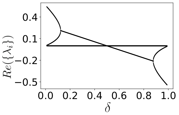
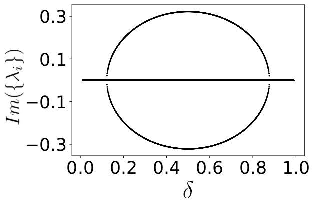
The conditions of Eq.(IX) is actually valid as a steady state , i.e., it is a solution of the dynamical equations. However, depending on it does not characterizes the dynamics of the system, since it becomes an unstable fixed point. In order to highligh it we show in Fig.(9)-(upper panels) the Jacobian spectrum for such steady states. While it is an attractor for , it becomes a repulsor for (or an unstable steady state). At the transition point the full spectrum has only imaginary terms.
Phase II: for couplings and , we obtain the following steady state attractor,
| (41) |
We show in Fig.(8) the occupation numbers along this phase. The steady states do not depend on the coupling and the occupation numbers for energy levels and are now equal, with a nonzero occupation for energy level .
Similar to phase I, the conditions of Eq.(IX) is valid as a steady state for a larger range in the phase diagram, specifically, it is a solution of the dynamical equations with , though not always stable. In Fig.(9)-(bottom panels) we show the Jacobian spectrum for such steady states. We see that it corresponds to a repulsor (unstable steady state) for , while becoming an attractor for . At the transition point the full spectrum also has only imaginary terms.


Phase III: for couplings and we observe a boundary time crystal with the appearance of limit-cycles in the dynamics. We show in Fig.(7)-(inset) the dynamics of occupation numbers for an illustrative case. We remark that for different initial states, we observed the same dynamical limit-cycle attractor. Interesting to notice that the time crystal occurs not only in the weak dissipative regime (), as in the case, but also in a region of the strong dissipative regime (), indicating greater robustness of the phase.
Critical line: for coupling and we observe a very peculiar behavior. As discussed, the steady states of Eqs.(IX) are solutions of the dynamical equations also for . In this case, however, its Jacobian spectrum has only imaginary terms, corresponding to center steady states. It indicates that for a given initial state close to these steady states, the dynamics should correspond to closed orbits, typical of the BTC’s found in the collective system. We find that this is indeed the case. We show in Fig.(10)-(upper left panel) the dynamics for two initial states close to the steady states of Eq.(IX) for . Both show closed, but different, orbits.
Considering the case of an initial condition far from these steady states, thus out of a Jacobian linear stability approach, we see now the existence of limit-cycles. We show in Fig.(10)-(bottom left panel) the dynamics for initial states with , for or , both featuring the same limit-cycle dynamics. We also observed that other different initial states may lead to even further different limit-cycles. We remark that for larger coherent coupling the limit-cycles are not so apparent anymore, mostly resembling as closed period orbits - there is no clear transient time in the dynamics towards the dynamical attractor. In this case it is not conclusive the existence of limit cycles, however it is still clear the presence of multiple time crystal dynamical attractors.
We study also the Lyapunov spectrum for this critical line, see Fig.(10)-(right panels). We obtain that the full Lyapunov spectrum for all these different initial conditions is zero, corroborating the expectation of multiple BTC’s.
.
X Conclusion
In this work we studied boundary time crystals in collective and level systems. We obtained that the BTC phase can appear in different forms for these different cases, highlighting a richer phenomenology for such dynamical phases. We first considered the model with presented in Iemini et al. 2018 and extended the analysis of its phase diagram, obtaining the full set of steady states combining analytical and algebraically (quasi-analytically) approaches, and further studying its Jacobian stability. The existence of BTC in the model is seen to be directly related to the presence of center fixed points. Moreover, we obtained analytically the effects of a specific symmetry breaking Hamiltonian term to the dynamics, showing that BTC’s are destroyed by such a perturbation in the model.
The analysis of the collective -level system, composed of a pair of collective interacting -level systems, showed even more fruitful. The model supports more robust forms of BTC’s, from limit-cycles to period doubling bifurcations leading to chaos. The BTC is robust to symmetry breaking Hamiltonian term in this case. We obtained the orbit diagram of the model from its collective magnetization and extracted its bifurcation ratio for a finite . The bifurcation ratio for finite was found different from the Feigenbaum constant of the seminal logistic map. A careful analysis for the ratio in the limit remains as an interesting perspective for a future work.
In the collective -level system we observed that depending on the competition between the two Lindbaldians and the model supports static steady states characterized by a “dark level”, limit-cycle dynamics or a peculiar dynamical phase at the critical line where the strength of both channels are equal. At this critical line the systems shows multiple limit-cycle attractors, depending on the initial condition, as well as different closed period orbits. The Jacobian spectrum has no real terms (only nontrivial imaginary part) in this phase, as well as its Lyapunov exponents are all zero.
This work opens different interesting perspectives, showing how collective models with high -level systems can support different forms of BTC’s with richer properties. It would be interesting e.g. to explore larger ’s and its implications to these phases, possible applications as well as a throughout analysis on the role of the global and dynamical symmetries for such models.
Acknowledgements
We acknowledge enlightening discussions with R. Fazio. F.I. acknowledges the financial support of the Brazilian funding agencies National Council for Scientific and Technological Development—CNPq (Grant No. -) and FAPERJ (Grant No. E-).
Appendix A Paramagnetic steady states ()
The paramagnetic fixed points of the -level collective model in Eqs.(2)-(3) are given by the algebraic condition,
| (42) |
and we recall that this fixed point solutions are physical steady state only if this geometrical place intersects the fixed norm circle , thus satisfying the conservation of the total spin. In this case the steady states come in pairs, as in the previous case, however we can have or pairs depending on the system parameters and - see Fig.(11) for illustrative cases. We also show in Fig.(12) the steady states magnetization for varying Hamiltonian parameters. Since we use the azimutal angle in the plane, , in order to completely describe the steady state. The steady state magnetization is independent of the field (Eq.(42)). We see that varying the field, both starting from a trivial () or time-crystal phase (), induces the appearance of new pairs of steady states on the plane.


Appendix B Stability analysis ()
A linear stability analysis of the fixed points of the model can be performed from an spectral analysis of the Jacobian matrix. The approach is a follows. We recall that the dynamical equations of motion of the system can be written as , with and a nonlinear function on the variables. We can define the displaced variables around the fixed points and perform a series expansion. We obtain that,
| (43) |
where denotes the transposed of the line vector , is a matrix (denoted as Jacobian matrix) with elements and the correction terms are quadratic on the displaced variables and can be neglected within a linear approximation. The effective dynamical equations of motion around the fixed point are in this way linear differential equations which can be solved by the eigenspectrum of the Jacobian matrix. The spectral properties of the Jacobian thus provide all information of dynamics around the fixed points, at first order level. Let us analyse in detail the Jacobian eigenvalues for the two different cases of fixed points in the model.
Ferromagnetic fixed points, : for the pair of fixed points of Eq.(13) we compute the eigenvalues using sympy package from python. We obtain that their eigenvalues are given by,
| (44) |
where,
| (45) |
Apart from the trivial null eigenvalue, we see that the nontrivial eigenvalue has always a real part. As a consequence the possible steady states of the model with are always hyperbolic fixed points.
Paramagnetic fixed points, : for the case with the Jacobian matrix is simplified and one can obtain analytically their eigenvalues, which have the form,
| (46) |
where,
| (47) |
In this case we see that the eigenvalues (apart from the trivial one) are purely real or imaginary, thus corresponding either to hyperbolic fixed points or centers.
Appendix C Non Hermitian Perturbation Theory
The Jacobian of the system in Sec.(V) is written as
| (48) |
where is the unperturbed Jacobian and
| (49) |
is the perturbation matrix. We study the effects of such perturbation in the spectral properties of the Jacobian using Perturbation Theory for general matrices Li et al. 2014, as follows. Any matrix has generalized right () and left () eigenvectors defined as,
| (50) |
where left and right eigenvectors obey the ortogonality property , and are the generalized eigenvectors. We assume that the eigenvalues are non-degenerated, and thus we are dealing with non-degenerate Perturbation Theory. Expanding the eigenvalues and eigenvectors in terms of the perturbative term , we can write then as,
| (51) |
where the index denotes the correction order in perturbation theory, i.e. corresponds to the eigenvalues and eigenvectors of the unperturbed Jacobian . Combining Eq.(48) and Eq.(51) into Eq.(50), one can find the recursive expressions for general ’th order corrections. In particular, the corrections to the eigenvalues of the Jacobian are given by,
| (52) |
Focusing on the first order terms () we thus find the equations for the perturbative eigenvalue corrections
| (53) |
Appendix D structure constants
h!
References
- (1)
- Iemini et al. (2018) F. Iemini, A. Russomanno, J. Keeling, M. Schirò, M. Dalmonte, and R. Fazio, Phys. Rev. Lett. 121, 035301 (2018), URL https://link.aps.org/doi/10.1103/PhysRevLett.121.035301.
- Goldenfeld (1992) N. Goldenfeld (1992).
- Sachdev (2000) S. Sachdev, Cambridge University Press (2000).
- Wilczek (2012) F. Wilczek, Phys. Rev. Lett. 109, 160401 (2012), URL https://link.aps.org/doi/10.1103/PhysRevLett.109.160401.
- Li et al. (2012) T. Li, Z.-X. Gong, Z.-Q. Yin, H. T. Quan, X. Yin, P. Zhang, L.-M. Duan, and X. Zhang, Phys. Rev. Lett. 109, 163001 (2012), URL https://link.aps.org/doi/10.1103/PhysRevLett.109.163001.
- Bruno (2013a) P. Bruno, Phys. Rev. Lett. 110, 118901 (2013a), URL https://link.aps.org/doi/10.1103/PhysRevLett.110.118901.
- Bruno (2013b) P. Bruno, Phys. Rev. Lett. 111, 029301 (2013b), URL https://link.aps.org/doi/10.1103/PhysRevLett.111.029301.
- Bruno (2013c) P. Bruno, Phys. Rev. Lett. 111, 070402 (2013c), URL https://link.aps.org/doi/10.1103/PhysRevLett.111.070402.
- Nozières, Philippe (2013) Nozières, Philippe, EPL 103, 57008 (2013), URL https://doi.org/10.1209/0295-5075/103/57008.
- Volovik (2013) G. Volovik, Jetp Lett. 98, 491–495 (2013), URL https://doi.org/10.1134/S0021364013210133.
- Watanabe and Oshikawa (2015) H. Watanabe and M. Oshikawa, Phys. Rev. Lett. 114, 251603 (2015), URL https://link.aps.org/doi/10.1103/PhysRevLett.114.251603.
- Russomanno et al. (2017) A. Russomanno, F. Iemini, M. Dalmonte, and R. Fazio, Phys. Rev. B 95, 214307 (2017), URL https://link.aps.org/doi/10.1103/PhysRevB.95.214307.
- Surace et al. (2019) F. M. Surace, A. Russomanno, M. Dalmonte, A. Silva, R. Fazio, and F. Iemini, Phys. Rev. B 99, 104303 (2019), URL https://link.aps.org/doi/10.1103/PhysRevB.99.104303.
- Sacha (2015) K. Sacha, Phys. Rev. A 91, 033617 (2015), URL https://link.aps.org/doi/10.1103/PhysRevA.91.033617.
- Syrwid et al. (2017) A. Syrwid, J. Zakrzewski, and K. Sacha, Phys. Rev. Lett. 119, 250602 (2017), URL https://link.aps.org/doi/10.1103/PhysRevLett.119.250602.
- Prokof’ev and Svistunov (2018) N. V. Prokof’ev and B. V. Svistunov, Journal of Experimental and Theoretical Physics 127, 860 (2018), URL https://doi.org/10.1134/S1063776118110092.
- Else et al. (2016) D. V. Else, B. Bauer, and C. Nayak, Phys. Rev. Lett. 117, 090402 (2016), URL https://link.aps.org/doi/10.1103/PhysRevLett.117.090402.
- Khemani et al. (2016) V. Khemani, A. Lazarides, R. Moessner, and S. L. Sondhi, Phys. Rev. Lett. 116, 250401 (2016), URL https://link.aps.org/doi/10.1103/PhysRevLett.116.250401.
- von Keyserlingk et al. (2016) C. W. von Keyserlingk, V. Khemani, and S. L. Sondhi, Phys. Rev. B 94, 085112 (2016), URL https://link.aps.org/doi/10.1103/PhysRevB.94.085112.
- Yao et al. (2017) N. Y. Yao, A. C. Potter, I.-D. Potirniche, and A. Vishwanath, Phys. Rev. Lett. 118, 030401 (2017), URL https://link.aps.org/doi/10.1103/PhysRevLett.118.030401.
- Ho et al. (2017) W. W. Ho, S. Choi, M. D. Lukin, and D. A. Abanin, Phys. Rev. Lett. 119, 010602 (2017), URL https://link.aps.org/doi/10.1103/PhysRevLett.119.010602.
- Huang et al. (2018) B. Huang, Y.-H. Wu, and W. V. Liu, Phys. Rev. Lett. 120, 110603 (2018), URL https://link.aps.org/doi/10.1103/PhysRevLett.120.110603.
- (24) B. Buča, J. Tindall and D. Jaksch, Nat Commun 10, 1730 (2019).
- Russomanno et al. (2020) A. Russomanno, S. Notarnicola, F. M. Surace, R. Fazio, M. Dalmonte, and M. Heyl, Phys. Rev. Research 2, 012003 (2020), URL https://link.aps.org/doi/10.1103/PhysRevResearch.2.012003.
- Khasseh et al. (2019) R. Khasseh, R. Fazio, S. Ruffo, and A. Russomanno, Phys. Rev. Lett. 123, 184301 (2019), URL https://link.aps.org/doi/10.1103/PhysRevLett.123.184301.
- Yao et al. (2020) N. Y. Yao, C. Nayak, L. Balents, and M. P. Zaletel, Nature Physics 16, 438 (2020), URL https://doi.org/10.1038/s41567-019-0782-3.
- Hurtado-Gutiérrez et al. (2020) R. Hurtado-Gutiérrez, C. F. Carollo, Pérez-Espigares, and P. Hurtado Phys. Rev. Lett. 125, 160601 2020 URL https://doi.org/10.1103/PhysRevLett.125.160601.
- Wang and Fazio (2021) P. Wang and R. Fazio, Phys. Rev. A 103, 013306 (2021), URL https://link.aps.org/doi/10.1103/PhysRevA.103.013306.
- Piccitto et al. (2021) G. Piccitto, M. Wauters, F. Nori, and N. Shammah (2021), URL arXiv:2101.05710.
- Riera-Campeny et al. (2020) A. Riera-Campeny, M. Moreno-Cardoner, and A. Sanpera, Quantum 4, 270 (2020), ISSN 2521-327X, URL https://doi.org/10.22331/q-2020-05-25-270.
- Lazarides et al. (2020) A. Lazarides, S. Roy, F. Piazza, and R. Moessner, Phys. Rev. Research 2, 022002 (2020), URL https://link.aps.org/doi/10.1103/PhysRevResearch.2.022002.
- Lledó and Szymańska (2020) C. Lledó and M. H. Szymańska, New Journal of Physics 22, 075002 (2020), URL https://doi.org/10.1088/1367-2630/ab9ae3.
- Seibold et al. (2020) K. Seibold, R. Rota, and V. Savona, Phys. Rev. A 101, 033839 (2020), URL https://link.aps.org/doi/10.1103/PhysRevA.101.033839.
- Marino et al. (2021) K. Seetharam, A. Lerose, R. Fazio, and J. Marino (2021), URL arXiv:arXiv:2101.06445).
- Zhang (2017) J. e. a. Zhang, Nature 543 (2017), URL https://doi.org/10.1038/nature21413.
- Choi (2017) S. e. a. Choi, Nature 543 (2017), URL https://doi.org/10.1038/nature21426.
- Rovny et al. (2018a) J. Rovny, R. L. Blum, and S. E. Barrett, Phys. Rev. Lett. 120, 180603 (2018a), URL https://link.aps.org/doi/10.1103/PhysRevLett.120.180603.
- Rovny et al. (2018b) J. Rovny, R. L. Blum, and S. E. Barrett, Phys. Rev. B 97, 184301 (2018b), URL https://link.aps.org/doi/10.1103/PhysRevB.97.184301.
- Pal et al. (2018) S. Pal, N. Nishad, T. S. Mahesh, and G. J. Sreejith, Phys. Rev. Lett. 120, 180602 (2018), URL https://link.aps.org/doi/10.1103/PhysRevLett.120.180602.
- Smits et al. (2018) J. Smits, L. Liao, H. T. C. Stoof, and P. van der Straten, Phys. Rev. Lett. 121, 185301 (2018), URL https://link.aps.org/doi/10.1103/PhysRevLett.121.185301.
- Sacha and Zakrzewski (2017) K. Sacha and J. Zakrzewski, Reports on Progress in Physics 81, 016401 (2017), URL https://doi.org/10.1088%2F1361-6633%2Faa8b38.
- Else et al. (2020) D. V. Else, C. Monroe, C. Nayak, and N. Y. Yao, Annual Review of Condensed Matter Physics 11, 467 (2020), URL https://doi.org/10.1146/annurev-conmatphys-031119-050658.
- Walls et al. (1978) D. F. Walls, P. D. Drummond, S. S. Hassan, and H. J. Carmichael, Progress of Theoretical Physics Supplement 64, 307 (1978), ISSN 0375-9687, eprint https://academic.oup.com/ptps/article-pdf/doi/10.1143/PTPS.64.307/5292058/64-307.pdf, URL https://doi.org/10.1143/PTPS.64.307.
- Drummond and Carmichael (1978) P. Drummond and H. Carmichael, Optics Communications 27, 160 (1978), ISSN 0030-4018, URL http://www.sciencedirect.com/science/article/pii/0030401878901980.
- Puri and Lawande (1979) R. Puri and S. Lawande, Physics Letters A 72, 200 (1979), ISSN 0375-9601, URL http://www.sciencedirect.com/science/article/pii/0375960179900033.
- Walls (1980) D. F. Walls, Journal of Physics B: Atomic and Molecular Physics 13, 2001 (1980), URL https://doi.org/10.1088/0022-3700/13/10/008.
- (48) S. Schneider and G. J. Milburn, Phys. Rev. A 65, 042107 (2002).
- (49) S. Morrison and A. S. Parkins, J. Phys. B: At. Mol. Opt. 41, 195502 (2008).
- Autti et al. (2020) S. Autti, P. J. Heikkinen, J. T. Makinen, G. E. Volovik, V. V. Zavjalov, and V. B. Eltsov, Nature Materials 20, 171–174 (2020), URL https://doi.org/10.1038/s41563-020-0780-y.
- Estarellas et al. (2020) M. P. Estarellas, T. Osada, V. M. Bastidas, B. Renoust, K. Sanaka, W. J. Munro, and K. Nemoto, Science Advances 6 (2020), eprint https://advances.sciencemag.org/content/6/42/eaay8892.full.pdf, URL https://advances.sciencemag.org/content/6/42/eaay8892.
- Yang and Cai (2021) X. Yang and Z. Cai, Phys. Rev. Lett. 126, 020602 (2021), URL https://link.aps.org/doi/10.1103/PhysRevLett.126.020602.
- Bomantara and Gong (2018) R. W. Bomantara and J. Gong, Phys. Rev. Lett. 120, 230405 (2018), URL https://link.aps.org/doi/10.1103/PhysRevLett.120.230405.
- Nielsen and Chuang (2000) M. Nielsen and I. Chuang, Quantum Computation and Quantum Information, Cambridge Series on Information and the Natural Sciences (Cambridge University Press, 2000), ISBN 9780521635035, URL https://books.google.com.br/books?id=65FqEKQOfP8C.
- (55) A. M. Chebotarev, Mathematical notes of the Academy of Sciences of the USSR 61, 510 (1997).
- (56) M. Gregoratti, Commun. Math. Phys. 222, 181 (2001).
- (57) J. Gough, Open Syst. Inf. Dyn. 22, 1550009 (2015).
- (58) J. Prior, A. W. Chin, S. F. Huelga, and M. B. Plenio, Phys. Rev. Lett. 105, 050404 (2010).
- (59) Javier Prior, Alex W. Chin, Susana F. Huelga and Martin B. Plenio, Phys. Rev. Lett. 105, 050404 (2010). R. Rosenbach, J. Cerrillo, S. F. Huelga, J. Cao, and M. B. Plenio, New. J. Phys. 18, 023035 (2016).
- (60) See also Supplementary Information “From Hamiltonian Dynamics to the Master Equation” of Ref.[].
- (61) S. Puri, C. K. Andersen, A. L. Grimsmo, and A. Blais, Nat. Commun. 8, 1 (2017).
- (62) L. Henriet, L. Beguin, A. Signoles, T. Lahaye, A. Browaeys, G.-O. Reymond, and C. Jurczak, Quantum 4, 327 (2020).
- (63) A. Angerer et al., Nat. Phys. 14, 1168 (2018).
- Hannukainen and Larson (2018) J. Hannukainen and J. Larson, Phys. Rev. A 98, 042113 (2018), URL https://link.aps.org/doi/10.1103/PhysRevA.98.042113.
- (65) F. Benatti, F. Carollo, R. Floreanini and H. Narnhofer, J. Phys. A: Math. Theor. 51 (2018) 325001.
- Pikovsky and Politi (2015) A. Pikovsky and A. Politi, Cambridge University Press (2015), URL http://dx.doi.org/10.1017/CBO9781139343473.
- Li et al. (2014) A. C. Y. Li, P. F., and K. Jens, Scientific Reports 4, 4887 (2014), URL https://doi.org/10.1038/srep04887.
- not (A detailed analysis of the initial state dependence is an interesting topic. It is, however, beyond the scope of this work) (A detailed analysis of the initial state dependence is an interesting topic. It is, however, beyond the scope of this work).
- Benettin et al. (1976) G. Benettin, L. Galgani, and J.-M. Strelcyn, Phys. Rev. A 14, 2338 (1976), URL https://link.aps.org/doi/10.1103/PhysRevA.14.2338.
- Benettin et al. (1980) G. Benettin, L. Galgani, A. Giorgilli, and J.-M. Strelcyn, Meccanica 15, 21 (1980), URL https://doi.org/10.1007/BF02128237.
- Sandri (1996) M. Sandri, The Mathematica Journal 6, 78 (1996).
- (72) Guido Homann, Jayson G. Cosme and Ludwig Mathey, Phys. Rev. Research 2, 043214 (2020).