Growth Functions, Rates and Classes of String-Based Multiway Systems

Consider a string-based multiway system $M$ (definition 10 in [5]), represented as a triplet $(R,s_{\text{init}},\Sigma)$ where $\Sigma$ is a finite alphabet, $R=\{r_{1}\rightarrow t_{1},\dots,r_{n}\rightarrow t_{n}\}$ is a set of string replacement rules over $\Sigma$ and $s_{\text{init}}\in\Sigma^{*}$ is the initial string³³ 3 In the following, $\Sigma^{*}$ denotes the set of all words over the alphabet $\Sigma$.. We define the “state-set of generation $n$” as the set of all new (previously nonexistent) states added to the multiway system in its $n$-th generation. These states are precisely the nodes of the states graph (c. f. section 5.3 in [21]) to which the shortest path from the initial state has length $n$. In [21] they are called “merged states”. Now, the “growth function⁴⁴ 4 We use the terms ‘sequence’ and ‘function’ interchangeably for $f:\mathbb{N}_{+}\rightarrow\mathbb{N}_{+}$.” $g_{M}(n)$ is simply the cardinality of the state-set of generation $n$.

In general, it is very hard or even undecidable (see section 3.3) to prove that some multiway system has a certain growth function. It is also not obvious that the growth functions of multiway systems should be elementary functions or “simple” by any other definition. Examples of systems where the growth function is hard to describe were already given in “A New Kind of Science” ([22] pp. 204 ff.). Therefore, we will approximate the growth functions of multiway systems by continuous, strictly monotonically increasing, unbounded (and hence bijective on $\mathbb{R}_{\geq 0}$) functions which can be analysed more easily. This way, many similar growth functions will be considered members of the same equivalence class. We will say that the corresponding multiway systems have the same “growth rate”.

To formalize the notion of approximating functions, we use the asymptotic growth classes from complexity theory, defined in the following way: For a function $f:A\rightarrow B$ where $A=B=\mathbb{R}_{\geq 0}$ or $A=B=\mathbb{R}$, $\mathcal{O}(f)$ is defined as the set of functions $g:A\rightarrow B$ for which $\limsup_{x\rightarrow\infty}|\frac{g(x)}{f(x)}|$ exists and is a real number⁵⁵ 5 An equivalent definition is $g\in\mathcal{O}(f)\iff\exists C\in\mathbb{R}_{+}:\exists x_{0}\in A:\forall x>x_{0}:C|f(x)|\geq|g(x)|$.. The subset of $\mathcal{O}(f)$ for which the limit superior is zero is denoted $o(f)$. Similarly, $\Omega(f):=\{g:A\rightarrow B\mid f\in\mathcal{O}(g)\}$ and $\omega(f):=\{g:A\rightarrow B\mid f\in o(g)\}$. Finally, $\Theta(f):=\Omega(f)\cap\mathcal{O}(f)$. It is straightforward to show that $f\sim_{\Theta}g\iff f\in\Theta(g)$ is an equivalence relation. Thus, we may speak of functions that are “asymptotically equal”.

As mentioned above, we want to approximate growth functions by bijective functions for the subsequent mathematical analysis. For some multiway growth function $a$, we will define the sequences $\overline{a}$ and $\underline{a}$ as its tightest upper and lower bounds which are monotonically increasing, even if $a$ itself is not monotonic at all. From these sequences, we will then construct two equivalence classes of continuous functions which are all asymptotically equal to and hence “close approximations” of $\overline{a}$ or $\underline{a}$ respectively. Two representatives of these classes will be called “tight bounds” and, since we are generally concerned with unbounded growth functions⁶⁶ 6 Bounded growth functions will be discussed shortly., both bijective on $\mathbb{R}_{\geq 0}$.

Notice that we have only defined asymptotic growth classes for functions on $\mathbb{R}$ or $\mathbb{R}_{\geq 0}$. However, since the multiway growth function is always a function on $\mathbb{N}_{+}$, we consider its linear interpolation, a continuous function from $\mathbb{R}_{\geq 0}$ to $\mathbb{R}_{\geq 0}$ which is equal to the sequence for natural arguments and always bounded by consecutive values of the sequence (see definition 2.2), instead.

One might ask why we introduce an upper and a lower bound instead of approximating the growth function with a single function. Doing so would however be a poor approximation as there are multiway systems for which even the tightest upper and lower bounds are never in the same asymptotic growth class (compare figure 4). We will call these multiway systems “strongly oscillating” and all others (i. e. systems where all tight bounds are asymptotically equal) “regular”. Notice that for every regular multiway system, a pair of bijective tight bounds exists because its tight bounds will be in the asymptotic equivalence class of two unbounded strictly monotonically increasing functions and tight bounds are continuous on $\mathbb{R}_{+}$. Strongly oscillating systems on the other hand are much more difficult to analyse since one cannot easily come up with criteria for measuring the rate of oscillation and it is not clear at all whether there has to be any periodicity or regularity in the way in which they oscillate. Thus, for our basic investigations about the fundamental structure of multiway systems, we shall focus on regular systems.

Definition 1.2 suggests a natural way to define classes of multiway systems with “similar” growth functions by considering growth functions with approximately equal tight bounds as equivalent. Let $f,g:\mathbb{N}_{+}\rightarrow\mathbb{N}_{+}$ be functions and $(a_{1},b_{1}),(a_{2},b_{2})$ be tight bounds of $f$ and $g$ respectively. We define $\sim_{R}$ by $f\sim_{R}g\iff(a_{1}\sim_{\Theta}a_{2}\land b_{1}\sim_{\Theta}b_{2})$. Since tight bounds always exist, $\sim_{R}$ is an equivalence relation because $\sim_{\Theta}$ is one. For some multiway system $M$ with growth function $g_{M}$, we call the equivalence class of $\sim_{R}$ that $g_{M}$ falls into the “growth rate” of $g_{M}$ (or sometimes the growth rate of just $M$).

It is obvious that every multiway system has exactly one growth function and exactly one growth rate. The converse, i. e. that every function $f:\mathbb{N}_{+}\rightarrow\mathbb{N}_{+}$ is the growth function of some multiway system or, respectively, that every pair of bijective functions on $\mathbb{R}_{\geq 0}$ is a pair of tight bounds of some multiway growth function, is clearly not true as emphasized in lemma 2.1. However, if we define much more general classes of growth functions which we will call “multiway growth classes”, we will see (in theorem 3.1) that they indeed partition the set of all multiway systems into a finite set of infinite subsets.

To further distinguish between types of multiway systems on a more abstract level and demonstrate which kinds of growth functions can be achieved, we want to define very broad classes of multiway systems whose growth functions show similar behavior on a large scale. We have already distinguished between finite, bounded and unbounded systems, as well as dividing the latter into regular and strongly oscillating systems. As outlined above, we will focus on regular systems. To group these into sets of systems of similar behavior, we use commonly known classes of functions such as polynomial or exponential functions⁷⁷ 7 Actually, we are talking about polynomially or, respectively, exponentially bounded functions which need not be polynomials or simple exponential functions., intermediately (faster than polynomial and slower than exponential) growing functions and some others.

More precisely: Let $G_{\text{pol}}$ be defined as the set of all continuous bijections $f:\mathbb{R}_{\geq 0}\rightarrow\mathbb{R}_{\geq 0}$ which satisfy $f\in\Omega(x^{n})\cap\mathcal{O}(x^{n+1})$ for some $n\in\mathbb{N}_{+}$ and define $G_{\text{exp}}$ as $\{f:\mathbb{R}_{\geq 0}\rightarrow\mathbb{R}_{\geq 0}\mid f\in\Omega(a^{x})\cap\mathcal{O}((a+1)^{x})\}$ for some $a\in\mathbb{N}_{>1}$. Similarly, let $G_{\text{supexp}}$ be the set $\{f:\mathbb{R}_{\geq 0}\rightarrow\mathbb{R}_{\geq 0}\mid\forall g\in G_{\text{exp}}:f\in\omega(g)\}$ where $f$ must be continuous and bijective. Additionally, denote by $G_{\text{int}}$ the set of all continuous bijections $f:\mathbb{R}_{\geq 0}\rightarrow\mathbb{R}_{\geq 0}$ fulfilling $\forall g\in G_{\text{pol}},h\in G_{\text{exp}}:f\in\omega(g)\cap o(h)$. Now, it is easy to define $G_{\text{invpol}}:=\{f\mid f^{-1}\in G_{\text{pol}}\}$, $G_{\text{invexp}}:=\{f\mid f^{-1}\in G_{\text{exp}}\}$, $G_{\text{invsupexp}}:=\{f\mid f^{-1}\in G_{\text{supexp}}\}$ and $G_{\text{invint}}:=\{f\mid f^{-1}\in G_{\text{int}}\}$.

These eight sets give a partition of the set of all continuous bijections on $\mathbb{R}_{\geq 0}$ because a function grows either slower than $f:x\mapsto x$ in which case its inverse grows faster than $f$, or it grows faster (or equal to) $f$ in which case it is contained in one of the first four classes. We call a multiway system a member of the growth class $C_{i}$ if its growth function has tight bounds $f,g$ belonging⁸⁸ 8 This definition applies only to regular multiway systems to $G_{i}$. However, as definition 1.2 is not applicable for finite or bounded multiway systems, we handle them separately.

Let $C_{\text{fin}}$ and $C_{\text{bnd}}$ the sets of all finite and bounded multiway systems respectively. For all multiway systems in $C_{\text{fin}}\cup C_{\text{bnd}}$, the growth rate is defined to be $(1,1)$. While finite and bounded systems can have quite an intricate structure⁹⁹ 9 In fact, what seems to be “complex behavior” in a “New Kind of Science”-fashion (compare [22]), occurred much more frequently in our empirical investigations of finite systems but this might just indicate a lack of understanding., their growth functions are not very interesting for our purposes. They might be useful for applications not directly related to the Wolfram Physics Project, but in this paper, they will not be discussed in great detail.

As every continuous bijection on $\mathbb{R}_{+}$ belongs to exactly one of the $G_{i}$, every multiway system one can imagine is either strongly oscillating or in one of those classes (including $C_{\text{fin}}$ and $C_{\text{bnd}}$). We will furthermore show in theorem 3.1 that every of these classes (except $C_{\text{supexp}}$ which is empty by lemma 2.1) contains infinitely many multiway systems.

Summarizing the previous section, we introduced the three main concepts of multiway growth functions, multiway growth rates and multiway growth classes. We will now present the first important result of this paper, a theorem about the boundaries of possible growth rates, and spend the next section proving and illustrating it.

Now let us formalize the proof outlined above. For some function $T:\mathbb{N}\rightarrow\mathbb{N}$, we define a “$T$-halter” to be a Turing machine $\mathcal{T}$ such that $\mathcal{T}$ executes precisely $T(n)$ operations when given the input $n$, taking into account the input and output constraints depicted in figure 6(a). These constraints will later allow us to “enchain” the multiway systems corresponding to $T$-halters. Of course, neither is there a $T$-halter for arbitrary $T$ nor must there be a unique $T$-halter for a given $T$. However, and this is the part we care about, there is a $T$-halter such that $T\in\Omega(f)$ for any computable function $f$ because we can just take the Turing machine that computes $f$ and add some logic to write $n+1$ after the computation is finished.

Having defined $T$-halters, the next step is to show how multiway systems can emulate these (and all other Turing machines). Since we are talking about deterministic Turing machines, no branching shall occur in the corresponding multiway system, i. e. the system should have exactly one state in generation $n$ which corresponds to the state of the Turing machine after $n-1$ operations. Because at every state in the machine’s evolution only a finite part of the tape contains non-blank symbols, we include only the symbols already “touched” by the machine (meaning the head was on that symbol at least once) in the states of the multiway system and abbreviate the infinite strings of zeros on both sides of the tape with an underscore. The position and state of the head are indicated by an $H$ right of the symbol the head is currently on, followed by the current state number. Hence, there are four additional symbols (two underscores, an $H$ and a number) used in the multiway system but not written on the machine’s tape (see figure 6(b)).

Using this representation, plain read/write operations and state changes would be straightforward to implement as replacement rules, as we could just introduce a rule¹¹¹¹ 11 Writing symbols next to each other in this contexts simply denotes their concatenation to a string. $``xHn"\rightarrow``yHm"$ for every combination of currently read symbol $x$ and head state $n$. However, since the head must move left or right after each such operation, those rules are not suitable. What is needed instead to encode the operation “when $x_{1}$ is read in state $n$, write $y_{1}$, change state to $m$ and move the head right”, is a rule of the form $``x_{1}Hnx_{2}"\rightarrow``y_{1}x_{2}Hm"$ for every possible value of $x_{2}$. Similarly, a left move of the head is encoded as $``x_{2}x_{1}Hn"\rightarrow``x_{2}Hmy_{1}"$. If $n$ is not a halting state (in which case we would not need any rules), exactly one of these two rule patterns will be applicable for every possible value of $x_{1}$ or, respectively, every state transition arrow starting at $H$ in the state transition diagram.

For a Turing machine with $N$ states working on an alphabet of $S$ symbols, that already gives a worst-case (no halting states) of $N\cdot S^{2}$ rules in the corresponding multiway system. However, $N\cdot S$ (worst-case) more rules have to be added to handle the literal “edge cases” in which the head is next to one of the underscores bounding the tape. The two rule patterns, of which, as before, exactly one will match for every state transition arrow, are $``\_xHn"\rightarrow``\_0Hmy"$ for a left move and $``xHn\_"\rightarrow``y0Hm\_"$ for a right move (in both cases $x$ is read and $y$ written). Now, the resulting rule set captures all of the Turing machine’s properties and is able to extend the tape to any required length by itself. As an initial state of the multiway system to emulate the machine, any string of characters from the machines alphabet together with an $``Hs"$ where $s$ is the starting state and the two bounding underscores can be used.

To illustrate this construction, consider the Turing machine $\mathcal{T}_{1}$ shown in figure 7(a). It is, in some sense, the easiest possible $T$-halter for it does nothing more than increasing the number on the tape by one and placing its head back at the beginning. Figure 6(b) shows the successive states of the machine (and tape) next to a multiway system $M_{1}$ emulating $\mathcal{T}_{1}$. The rule set for this specific instance is

{"00H1" -> "0H21", "10H1" -> "1H21", "1H10" -> "10H1", "1H11" -> "11H1",
 "01H2" -> "0H21", "11H2" -> "1H21", "0H20" -> "00H3", "0H21" -> "01H3",
 "_0H1" -> "_0H21", "1H1_" -> "10H1_", "_1H2" -> "_0H21", "0H2_" -> "00H3_"}

Now it is clear that a multiway system emulating some $T$-halter $\mathcal{T}$ has exactly one state for $T(n)$ generations when started with the initial condition $``\_1H11^{n-1}\_"$ ($1^{n-1}$ denotes $n-1$ times the symbol $1$, the first $1$ is left of the head and the head starts in state 1). Now, we need a way to “enchain” this multiway system with itself. To achieve this, first add the rules $``Hf"\rightarrow``X"$ for every halting state $f$ where $X$ is one fixed symbol not contained in $\mathcal{T}$’s alphabet. These additional rules will cause the multiway state in generation $T(n)+1$ to look like $``\_w_{1}01X1^{n}0w_{2}\_"$¹²¹² 12 If the head is left of the first digit, $``\_w_{1}0X1^{n+1}0w_{2}\_"$ works analogously. where $w_{1}$ and $w_{2}$ are arbitrary words that might be created as byproducts in the working of $\mathcal{T}$. This is due to the $T$-halter constraints depicted in figure 6(a) or, rather, the $T$-halter constraints were chosen precisely to cause such a configuration of the tape.

Adding the rules $``X1"\rightarrow``1X"$, $``X0"\rightarrow``Y\_0"$, $``1Y"\rightarrow``Y1"$ and $``0Y1"\rightarrow``0\_1H1"$ will cause exactly one state where the $X$ has “moved” one position to the right for $n$ generations (first rule), then add an underscore behind the $n$ ones (second rule), “move back to the left” using the $Y$ for $n+1$ generations (third rule) and finally add an underscore at the left side, replacing $Y$ by the starting state symbol $``H1"$ of $\mathcal{T}$ (see figure 7(b)). Now, the whole process can start again because the new underscores ensure a “fresh” new tape for $\mathcal{T}$ which now contains, by the $T$-halter constraints, $n+1$ as the next input for $\mathcal{T}$ to continue with while everything outside the bounding underscores will be ignored.

The resulting multiway system of this continued re-evaluation of $\mathcal{T}$ will run indefinitely, subsequently running instances of $\mathcal{T}$ with larger and larger values of $n$. Despite that, it still has only one state in all generations. In order to make the number of states increase exactly when $n$ increases, i. e. some instance of $\mathcal{T}$ finished working, we add the rules $``0Y1"\rightarrow``Z"$ and $``Z"\rightarrow``ZZ"$. This way, the multiway states graph branches every time the system starts a new instance of $\mathcal{T}$ into a main branch where the evaluation of $\mathcal{T}$ continues and a diverging branch where the second rule just creates longer and longer strings of $Z$’s forever, constantly adding one new state to every generation. Thus, the number of divergent branches is always equal to $n-1$ and these branches grow constantly forever, causing the desired behavior as shown in figure 7(b).

As it takes a “preparation time” of $p(n)=2(n+1)+1$ steps (the head moves over $n+1$ symbols¹³¹³ 13 If the head starts at the left of the first digit instead, the formula is $p(n)=2(n+2)$., including the new 1) before the $n+1$-th iteration of $\mathcal{T}$ can start after the $n$-th iteration is done, there will be $n$ states for $T(n)+p(n)$ steps in the multiway system constructed above, before the number of states increases by one. Let us generally investigate the sequences obtained this way:

Since definition 2.1 requires $f$ to be always greater than zero, every natural number can be represented as some sum over consecutive values of $f$ plus a remainder and, as figure 8(a) shows, this definition indeed matches the informal description of “$n$ occurs $f(n)$ times”. Notice as well that the linear interpolation, despite being defined as a curve in $\mathbb{R}^{2}$, can be regarded as a continuous function from $\mathbb{R}_{\geq 0}$ to $\mathbb{R}_{\geq 0}$ because for all $n\in S$, the function to be interpolated assigns precisely one $y$-value and since $S$ is an infinite subset of $\mathbb{N}$, the linear interpolation function is defined everywhere on $\mathbb{R}_{\geq 0}$.

Now, to express some sequence $A_{f}$ explicitly, define the set of increase-indices of $A_{f}$ as $I(A_{f}):=\{n\in\mathbb{N}_{+}\mid A_{f}(n-1)<A_{f}(n)\}$. It follows that $L_{I(A_{f})}(A_{f})$ will always be strictly monotonically increasing and unbounded. Therefore, its inverse function $L_{I(A_{f})}(A_{f})^{-1}$ exists and we can formulate the following lemma:

Putting it all together, we conclude from the previous Turing machine investigation that for every halting function $T\in\Omega(n)$, there is a multiway system which has the growth function $g_{M}(n)=A_{T+p}(n)$ for some $p\in\Theta(n)$. Additionally, as $p$ “delays” the growth function even more¹⁴¹⁴ 14 Since $p\in\Theta(n)$, $g_{M}$ will even become strictly less than $L_{\mathbb{N}_{+}}(T_{\sigma})^{-1}$ very soon. In most practical cases, $g_{M}$ is much lower., i. e. $\forall n\in\mathbb{N}_{+}:A_{T+p}(n)\leq A_{T}(n)$, it follows that

by lemma 2.2, which proves theorem 2.1.

Computing linear interpolations and their inverse functions seems hard to do analytically because in most cases, there are no elementary closed-form expressions describing them. Therefore, it might seem difficult to actually apply theorem 2.1. However, since we are only interested in growth rates, we can use approximations to make calculations much more easy.

Whenever it is possible to express some halting function in a closed form (e. g. $T:\mathbb{N}_{+}\rightarrow\mathbb{N}_{+},n\mapsto 2n^{2}+3n$) which could also describe a bijective function on $\mathbb{R}_{\geq 0}$ (like $f(x)=2x^{2}+3x$), we can use the lemma above to simplify calculations: Since $f$ is monotonically increasing and the linear interpolation equals the summatory function for natural arguments, we have

Therefore, lemma 2.3 tells us that we can approximate the inverse of the summatory function used in theorem 2.1 just by computing the inverse of the integral of $f$. Especially in the case of logarithms or exponential functions, solving integrals is much easier than computing sums, so this lemma can be very useful.

To demonstrate this and assist the proof of theorem 3.1, let us imagine we wanted to construct a multiway system of logarithmic growth rate. We can approach this problem by designing a $T$-halter for some $T_{\text{exp}}\in\Theta(2^{n})$ and implementing the construction described in section 2.1 to get a multiway system with the inverse growth rate. As an example, take the Turing machine $\mathcal{T}_{\text{exp}}$ shown in figure 9. It is started in state 1 which simply moves the head to the right end of the word on the tape and changes to state 2. In this state, the head moves left again, replacing 2’s by 1’s until it encounters a 1, which it changes to a 2 and returns to state 1, repeating the process. It is easy to see that this is precisely the process of incrementing a binary number where 1 corresponds to a zero and 2 to a one. The process is repeated until the head moves to the left of the word, which, by then, consists only of 1’s since the previous string was the symbol $2$ repeated $n$ times. When the head encounters the first blank symbol on the left, it writes one more 1 to satisfy the $T$-halter constraint of incrementing the unary number, and then halts. The process is shown in figure 9 for $n=3$.

Consider the action of the machine when started at the right of some binary word of 1’s and 2’s in state 1: The head moves $b$ symbols to the left until it encounters the rightmost 1, and then $b$ symbols back after changing it. Since there are $2^{n-b}$ binary words of length $n$ where the rightmost $1$ is at position $b$, the Turing machine takes

steps before the head is at the right of $1^{n}$ and in state 1. Since the machine takes $n+2$ steps to move to the left again, write the new 1 and halt, as well as taking $n$ steps to move the head to the right in the first place, the total number of states, including starting and halting state, simplifies to

In combination with lemma 2.3, another strategy for simplifying calculations is to give easily computable bounds for $T$. In this case, we use the fact that $2^{n+1}<2^{n+2}-1<2^{n+2}$ for all $n\in\mathbb{N}$ to obtain $2^{x+1}<L_{\mathbb{N}_{+}}(T_{\text{exp}})(x)<2^{x+2}$ for all $x\in\mathbb{R}_{\geq 0}$. Letting $l(x):=L_{\mathbb{N}_{+}}(T_{\text{exp}})(x)$ for readability, this becomes

Since the inverse of $x\mapsto\frac{a}{\ln(2)}(2^{x}-1)$ is $y\mapsto\log_{2}(y\frac{\ln(2)}{a}+1)$, and $f(x)<g(x)\iff f^{-1}(x)>g^{-1}(x)$, the equation is equivalent to

Now, notice that

and

From this, we know $(\int_{0}^{x}l(t)\,\mathrm{d}t)^{-1}\in\Theta(\log_{2}(x))$ because the upper and lower bound asymptotically equal $\log_{2}(x)$. By lemma 2.3 and equation 7, $(\int_{0}^{x}l(t)\,\mathrm{d}t)^{-1}$ is also in $\Theta(L_{I(A_{T_{\text{exp}}})}(A_{T_{\text{exp}}}))$ and we can conclude that $A_{T_{\text{exp}}}\sim_{\Theta}\log_{2}(x)$. Simulating the multiway system and measuring the growth function empirically supports this as figure 10 shows. In future examples, most steps of the argumentation presented here can be shortened. However, this method of estimation does not work in all cases because the inverse bounds might not accurate enough to be asymptotically equal¹⁵¹⁵ 15 It is not true in general that $f\in\Theta(g)$ implies $f^{-1}\in\Theta(g^{-1})$. As a counter-example, consider $f(x)=\ln(x)$ and $g(x)=2\ln(x)$..

What we have seen in the above example is just a simple demonstration of the power of theorem 2.1. Besides from helping us later to prove theorem 3.1, it tells us a lot about the abstract structure of multiway growth function, their “growth spectrum”. By providing the following two corollaries, theorem 2.1 gives us knowledge about what this spectrum of possible growth rates looks like, i. e. which kinds of growth rates are possible and which kinds are not. In addition to that, it establishes connections between multiway growth functions and other classes of functions, namely computable functions and primitive recursive functions.

This quite remarkable fact also shows that for every multiway system growing faster than a bounded function, a more slowly growing multiway system exists because the growth function of every multiway system is obviously computable. We might therefore say that multiway systems can grow arbitrarily slowly, i. e. the set of regular multiway systems excluding constant and finite systems is “open” in some sense. Remember however that they cannot grow arbitrarily quickly as shown in lemma 2.1.

Let $M_{1}=(R_{1},s_{1},\Sigma_{1}),M_{2}=(R_{2},s_{2},\Sigma_{2})$ and $M_{3}=(R_{3},s_{3},\Sigma_{3})$ be multiway systems. Additionally, let $X$ be a unique (equal for all multiway systems) symbol not included in any multiway systems alphabet. Now, we define the “sum system” by $M_{1}\oplus M_{2}=(R_{1}\cup R_{2}\cup\{X\rightarrow s_{i}\mid s_{i}\in S_{2}(M_{1})\cup S_{2}(M_{2})\},``X",\Sigma_{1}\cup\Sigma_{2})$ where $S_{2}(M)$ is the state-set of $M$ in generation 2, i. e. all nodes with distance 1 to the initial state in the respective states graphs. The “product system” of $M_{1}$ and $M_{2}$ is now defined as $M_{1}\odot M_{2}=(R_{1}\cup R_{2},s_{1}s_{2},\Sigma_{1}\cup\Sigma_{2})$ where $s_{1}s_{2}$ denotes the concatenation of $s_{1}$ and $s_{2}$.

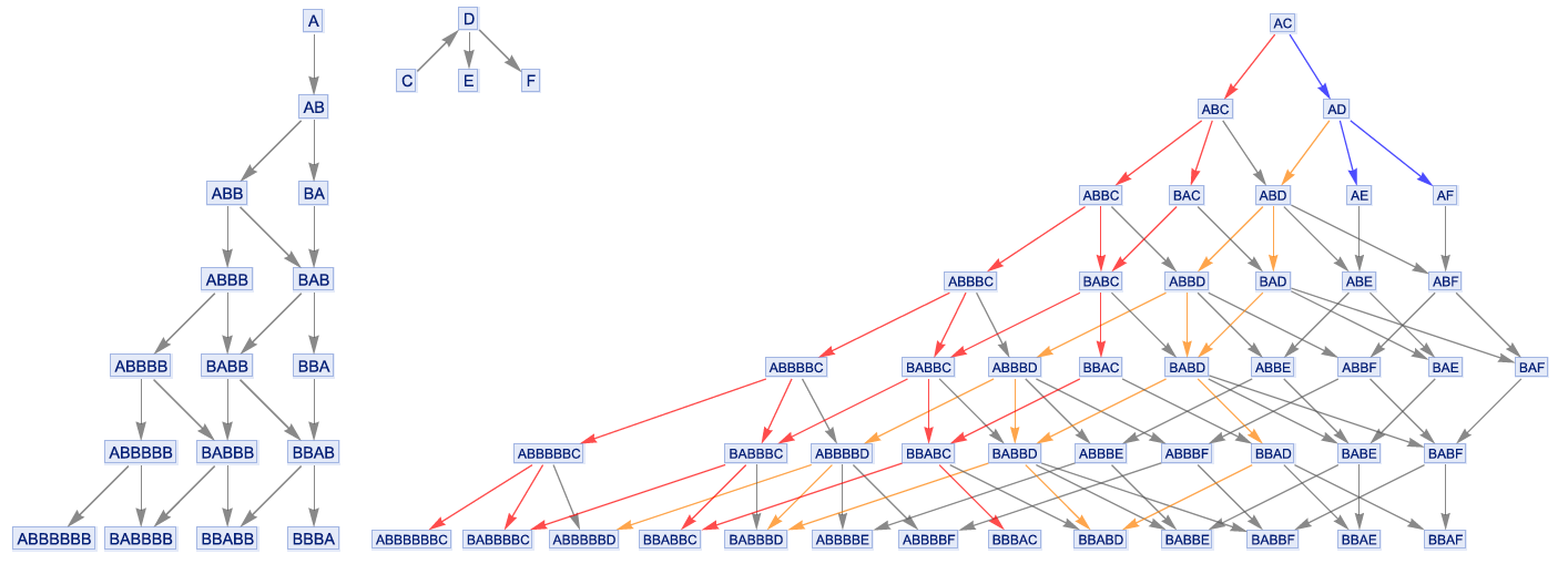
To calculate the growth functions of systems obtained by these operations, we shall require the parts $M_{1}$ and $M_{2}$ to be “rule independent” meaning that their rules do not interfere with each other. Formally, rule independence can be defined as the property that the states graph of $M_{1}$ is isomorphic to the states graph of $(R_{1}\cup R_{2},s_{1},\Sigma_{1}\cup\Sigma_{2})$, that is $M_{1}$ with all rules of $M_{2}$ added, and vice versa¹⁷¹⁷ 17 This works because if adding all the rules of $M_{1}$ to $M_{2}$ does not change its behavior, then these rules will not influence $M_{2}$’s states even if the states of $M_{1}$ get appended to them.. This property can always be achieved by requiring the underlying alphabets to be disjoint as in this case it will be impossible that a given string matches rules from $R_{1}$ and $R_{2}$ at the same time.

If we recall the definition of growth function $g_{M}(n)$ as the number of nodes to which the shortest path from the initial state has length $n$, it is easy to see that the growth function of $M_{1}\oplus M_{2}$ is one in the first iteration as $``X"$ is the only state. In further iterations, we can imagine a path of length $n$ simply as a path of length 1 entering either the states graph of $M_{1}$ or $M_{2}$, followed by a path of length $n-1$ originating at some state in the second layer of the chosen subgraph, as if the other graph was not there. This works because in the entire evolution, the initial state is the only one containing an $X$ so for all other states, the usual rules will apply and the rules replacing $X$ will have no effect. This concludes that the growth function of the sum system is precisely

References

- [1] D. Aggarwal “[Wolfram Winter School 2021] Multiway Systems as Cayley Graphs” URL: https://community.wolfram.com/groups/-/m/t/2162902
- [2] X.. Arsiwalla “[Wolfram Summer School 2020] Homotopic Foundations of Wolfram Models” URL: https://community.wolfram.com/groups/-/m/t/2032113
- [3] F. Baader and T. Nipkow “Term Rewriting and All That” USA: Cambridge University Press, 1998
- [4] N. Dershowitz “Term Rewriting Systems by “Terese” (Marc Bezem, Jan Willem Klop, and Roel de Vrijer, Eds.), Cambridge University Press, Cambridge Tracts in Theoretical Computer Science 55, 2003, Hard Cover: ISBN 0-521-39115-6, Xxii+884 Pages” In Theory Pract. Log. Program. 5.3 USA: Cambridge University Press, 2005, pp. 395–399 DOI: 10.1017/S1471068405222445
- [5] J. Gorard “Some Quantum Mechanical Properties of the Wolfram Model” In Complex Systems 29(2), 2020, pp. 537–598 URL: https://doi.org/10.25088/ComplexSystems.29.2.537
- [6] J. Gorard “Some Relativistic and Gravitational Properties of the Wolfram Model” In Complex Systems 29(2), 2020, pp. 599–654 URL: https://doi.org/10.25088/ComplexSystems.29.2.599
- [7] J. Gorard, M. Namuduri and X.. Arsiwalla “ZX-Calculus and Extended Hypergraph Rewriting Systems I: A Multiway Approach to Categorical Quantum Information Theory”, 2020 arXiv:2010.02752 [cs-dm]
- [8] J. Gorard, S. Wolfram and M. Piskunov “MultiwaySystem Resource Function” URL: https://resources.wolframcloud.com/FunctionRepository/resources/MultiwaySystem
- [9] R.. Grigorchuk “On the Milnor problem of group growth” In Soviet Math 28(1), 1983, pp. 23–26
- [10] A.. Hildebrand “Asymptotic Analysis Chapter 2 - Lecture Notes” In University of Illinois URL: https://faculty.math.illinois.edu/~hildebr/595ama/ama-ch2.pdf
- [11] Wolfram Inc. “Official Website of the Wolfram Physics Project” URL: https://www.wolframphysics.org/
- [12] Wolfram Inc. “Wolfram Functions Repository” URL: https://resources.wolframcloud.com/FunctionRepository
- [13] Y. Marji “[Wolfram Summer School 2020] Wolfram Models as Discretization Methods for Numerical PDE Solver” URL: https://community.wolfram.com/groups/-/m/t/2030068
- [14] A.. Meyer and D.. Ritchie “The complexity of loop programs” In ACM: Proceedings of the 22nd annual conference., 1967, pp. 465–469
- [15] M. Namuduri “[Wolfram Summer School 2020] Comparing Expansion in Physical and Branchial Space” URL: https://community.wolfram.com/groups/-/m/t/2029454
- [16] Y. Rabinovich “[Wolfram Summer School 2020] Shor’s Algorithm in Multiway Systems” URL: https://community.wolfram.com/groups/-/m/t/2029289
- [17] U. Storch and H. Wiebe “Lehrbuch der Mathematik - Band 1: Analysis einer Veränderlichen” Springer Spektrum, 2010
- [18] E.. Weisstein “”Figurate Number.” From MathWorld – A Wolfram Web Resource” URL: https://mathworld.wolfram.com/FigurateNumber.html
- [19] E.. Weisstein “”Graph Cartesian Product.” From MathWorld – A Wolfram Web Resource” URL: https://mathworld.wolfram.com/GraphCartesianProduct.html
- [20] E.. Weisstein “”Power Sum.” From MathWorld – A Wolfram Web Resource” URL: https://mathworld.wolfram.com/PowerSum.html
- [21] S. Wolfram “A Class of Models with the Potential to Represent Fundamental Physics” In Complex Systems 29(2), 2020, pp. 107–536 URL: https://doi.org/10.25088/ComplexSystems.29.2.107
- [22] S. Wolfram “A New Kind of Science” Wolfram Media, 2002 URL: https://www.wolframscience.com
- [23] S. Wolfram “A New Kind of Science, Notes for Section 5.6: Semigroups and groups [and multiway systems]” URL: https://www.wolframscience.com/nks/notes-5-6--semigroups-and-groups-and-multiway-systems/
- [24] S. Wolfram “A PROJECT TO FIND THE FUNDAMENTAL THEORY OF PHYSICS” Wolfram Media, 2020
- [25] S. Wolfram “Finally We May Have a Path to the Fundamental Theory of Physics… and It’s Beautiful”, 2020 URL: https://writings.stephenwolfram.com/2020/04/finally-we-may-have-a-path-to-the-fundamental-theory-of-physics-and-its-beautiful/