Microwave response of a chiral Majorana interferometer
Abstract
We consider an interferometer based on artificially induced topological superconductivity and chiral 1D Majorana fermions. The (non-topological) superconducting island inducing the superconducting correlations in the topological substrate is assumed to be floating. This allows probing the physics of interfering Majorana modes via microwave response, i.e., the frequency dependent impedance between the island and the earth. Namely, charging and discharging of the island is controlled by the time-delayed interference of chiral Majorana excitations in both normal and Andreev channels. We argue that microwave measurements provide a direct way to observe the physics of 1D chiral Majorana modes.
I Introduction
Physics of artificial topological superconductors with chiral Majorana edge modes was a subject of intensive research during the last decade Qi and Zhang 2011; Alicea 2012; Beenakker 2013; Kallin and Berlinsky 2016. Initially, these systems were proposed in hybrid structures on surfaces of topological insulators, covered by regular superconductors and magnetic insulators Fu and Kane 2008. Later on, heterostructures based on quantum anomalous Hall insulators (QAHI) combined with regular superconductors He et al. 2017; Shen et al. 2020 were experimentally studied. However, the reported evidence of the chiral Majorana fermions as half-quantized plateau in the two-terminal conductance He et al. 2017 is under debate Kayyalha et al. 2020. Further experimental advances were made in magnetic domains covered by superconducting monolayers Ménard et al. 2017 and in similar in spirit van der Waals heterostructures Kezilebieke et al. 2020 (see also a theoretical proposal Li et al. 2016). Surfaces of iron-based superconductors Wang et al. 2020 showed signs of topological superconductivity. Alternative realization of 1D Majorana edges in magnetic materials showing a spin liquid phase was reported in Kasahara et al. 2018.
Interferometers based on chiral Majorana modes should allow probing the nontrivial physics of these systems Fu and Kane 2009; Akhmerov et al. 2009; Strübi et al. 2015; Strübi et al. 2011; Li et al. 2012; Shapiro et al. 2016; Shapiro et al. 2017; Shapiro et al. 2018; Chung et al. 2011; Liu and Trauzettel 2011; Hou et al. 2013. The first proposals addressed the dc-transport Fu and Kane 2009; Akhmerov et al. 2009. Later, in a series of works the noise, braiding of Majorana edge vortices, and time resolved transport were studied Lian et al. 2018; Beenakker et al. 2019; Hassler et al. 2020; Beenakker and Oriekhov 2020; Adagideli et al. 2020.
Usually the regular superconductor, which induces the superconducting correlations in the topological material, is considered to have a fixed electrochemical potential. We, in contrast, consider a floating island. This allows us investigating the time resolved charging and discharging dynamics of the island, which can be measured using microwave experimental techniques.
II Qualitative picture
We consider a system depicted symbolically in Fig. 1(a). Here, a single Ohmic contact serves as a source and a drain of chiral Dirac modes. As the chiral Dirac mode approaches the superconducting area it is split into two chiral Majorana modes. The latter recombine later again into a chiral Dirac mode. We assume the lengths of the two Majorana branches, and , to be different, thus two different propagation times, and ( is a Fermi velocity of surface states in a topological material). These time intervals determine the Thouless energy, , and another energy, . The superconducting island is floating and is characterized by a self-capacitance or, equivalently, by the charging energy .

Below, using the effective action technique we derive the admittance (inverse impedance) of the island relative to the ground (source and drain), which is due to the currents in the edge modes. That is, corresponds to the admittance between points and in Fig. 1 (a) without the self-capacitance . The total admittance between points and in Fig. 1(a) is a sum of and that due to , i.e., . We obtain
| (1) |
where is the conductance quantum, is Boltzmann constant, is the temperature of a Fermi liquid in the Ohmic contact, and is a number of vortices in the superconducting island. In what follows, we set and restore them in final expressions.
To understand the physical meaning of the admittance it is useful to plot the response of the current flowing into the island to a voltage pulse applied to the contact of Fig. 1(a). This is, of course, given by , where is the Fourier image of . The responses to a delta-like and a step-like pulses at are depicted in Figs. 2(a) and 2(b), respectively.

The instantaneous response provided by the first term in Eq. (1) is explained by the immediate adjustment of the current in the outgoing Dirac mode to the new electrochemical potential of the island. This response corresponds to the effective conductance . The delayed response is due to the interference of the Majorana excitations created by the voltage pulse at . A similar effect (beyond the linear response analyzed here) was considered in Ref. Adagideli et al. 2020. The delayed response corresponds either to the normal or the Andreev reflection depending on the number of vortices in the island. In this chiral interferometer, the Andreev and normal reflections occur as a forward scattering from the incident into the outgoing Dirac channel. These are non-local in space and time processes with the amplitudes determined by the phases acquired by chiral Majorana excitations. Due to the spin texture of the Majorana modes a relative Berry phase is acquired in addition to the relative topological phase due to vortices in the superconductor. Hence, the Andreev reflection regime is associated with odd and the normal with even , . The response to the delta-functional pulse coincides with which is nothing but the interferometer Green function. A response to an arbitrary pulse is given by a convolution with .
We note that the floating phase can be gauged out from the superconductor into Dirac modes. We note a similarity with the description of the transport in terms of wavepackets induced by voltage pulses (sometimes called “levitons” Keeling et al. 2006). Namely, the immediate singular response in Fig. 2 (a) corresponds to an emission of a “leviton” into the outgoing chiral channel. The delayed one is a transfer of another “leviton” through Majorana edge modes.
At zero temperature, for the step-like voltage pulse the current finally stabilizes at the value corresponding to conductance in the Andreev reflection regime or in the normal reflection regime (see Fig. 2(b)). At finite , the conductance saturates at the values attenuated by thermal fluctuations, , with . At high temperatures, , we obtain , which corresponds to a completely suppressed interference between the two Majorana branches.
The ac response depends on both and , whereas, the dc response calculated in Refs.Akhmerov et al. 2009; Fu and Kane 2009 does not involve . We note that the admittance calculated here between points and assumes that the source and drain are grounded (see Fig. 1(a)). In Refs.Akhmerov et al. 2009; Fu and Kane 2009, the dc conductance was calculated in the alternative setting where the drain and the superconductor were grounded. The zero frequency limit for the admittance, , reproduces the results of those works for dc conductances in the linear response limit.
III Proposed measurement
We propose to couple the superconducting island to a microwave waveguide (transmission line), as shown in Fig. 1(b). One should be able to measure the reflection amplitude given by
| (2) |
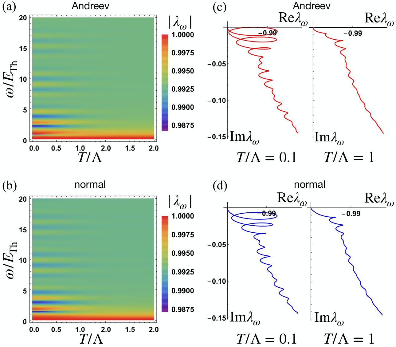
Here, is a transmission line impedance, which in an idealized situation approaches Ohm, the free space impedance. The experimentally relevant capacitances should be of the same order, . The reflection coefficient is close to . This means that the measured response is determined by the fine structure constant, , i.e., the effect is of the order of . The function shows decaying oscillations as a function of with periods proportional to and (see Figs. 3(a) and (b)). We mention that contemporary experimental methods allow to increase up to the resistance quantum, , and even higher. This is possible in superinductors realized as ladders of Josephson junctions Manucharyan et al. 2009; Bell et al. 2012 and high-kinetic-inductance materials Grünhaupt et al. 2018. Thus, the effect can be enhanced significantly.
Equation (2) allows one to extract from the experimental data for (and, thus, ). An observation of the delayed response can be a conclusive evidence of interfering Majorana fermions.
An observation of the delayed response can be disrupted by quasi-particle poisoning and by fluctuations of vortices parity. On the other hand, the random charge fluctuations, which are usually the main mechanism of the noise, do not pose any problem as they decouple in the linear response regime.
Two possible physical realizations of the interferometer are depicted in Fig. 4. The first realization is a QAHI film covered by a superconductor as shown in Fig. 4(a). The second realization is a 3D topological insulator covered with magnetic insulators of opposite magnetizations, and a superconductor (Fig. 4(b)).

IV A sketch of the derivation
IV.1 Limit of zero phase fluctuations: Scattering approach and effective action
We first describe the mean-field situation in which the superconducting order parameter does not fluctuate. Since we have just a single superconducting island we can assume to be real. The Bogoliubov-de Gennes equations describing setups like those in Fig. 4(b) have been extensively discussed in the literature Fu and Kane 2008; Fu and Kane 2009. At low energies, only the Dirac or Majorana edge modes are relevant since the bulk is gapped everywhere. For the Dirac edge mode, which emerges from the source, the action reads . For the relevant values of and (between the source and the first Y-splitting) the inverse propagator is obtained by the Fourier transform of
| (3) |
Here, is the equilibrium distribution function dictated by the Ohmic contact, and is an infinitesimal positive frequency. This is a matrix in the basis of the Keldysh space (Pauli matrices in this space are denoted by ) Kamenev 2011. Introducing the Nambu spinor we rewrite the action as , where and . The Pauli matrices act in the Gor’kov-Nambu particle-hole space and correspond to electron-like or hole-like state in the Dirac channel.
The scattering matrix for the lower (first) Y-splitting describes the conversion of an incident Dirac electron and hole into a pair of Majorana particles and :
| (4) |
The Hermitian conjugated of the upper (second) Y-splitting describes the conversion of Majorana modes into outgoing Dirac fermions: . Finally, a relation between in- and out- Dirac states and reads
| (5) |
Here, the scattering matrix is found as where determines Berry and topological phases, and dynamic phases of coherently propagating Majorana excitations.
With the help of the above introduced scattering matrix we now transform from the basis of incoming Dirac states to the basis of exact scattering states. That is, the field now annihilates an exact scattering state in the whole setup. The action retains its form, i.e.,
| (6) |
The scattering matrix allows us to represent the current flowing into the island, , as
| (7) |
where the matrix has a non-diagonal structure in momentum and Gor’kov-Nambu spaces.
IV.2 Regime of fluctuating phase: Gauge transform and derivation of the interaction part in the effective action
Next we allow the phase of the order parameter to fluctuate. The scattering of Dirac fermions becomes inelastic in this case; the energy-dependent Blanter and Büttiker 2000 scattering matrix obtains a non-stationary structure. Below we derive an interaction term in the action which couples fermion and boson degrees of freedom. We perform a standard gauge transformation of fermion phases Levitov et al. 1996; Andreev and Kamenev 2000; Kamenev 2011, which makes the superconducting order parameter real, . The Majorana edge modes are transformed accordingly and we extend the gauge transformation infinitesimally into the incoming and outgoing Dirac modes. That is
| (8) |
where is the coordinate of the first Y-splittings and at the later stage of the derivation. Similarly
| (9) |
where is the coordinate of the second Y-splitting. The discrete symmetry is preserved.
In the above discussed gauge transform, we encounter the theta-function regularization problem because we go beyond the long wave-length approximation. We resolve it using a discretized tight-binding approach. The derivation is based on four steps (i-iv) schematically illustrated in Fig. 5. Let us map chiral Dirac modes and onto a line with the coordinate (Fig. 5 (i)). The Y-splittings are located at , the incident mode scatters into a pair of Majorana modes surrounding the topological superconductor with floating phase of the order parameter, , which in turn fuse into .

In the second step (see Fig. 5 (ii)), we gauge out the superconducting phase, , in accordacne with Eqs. (8, 9). As mentioned, we extend the the step-like gauge transformation slightly beyond the superconductor, i.e., we perform it in the interval . This gives two phase drops at and , which are marked by red crosses.
In the third step we transform the chiral modes and to a non-chiral mode on a semi-axis (Fig. 5 (iii)). Both phase drops are now merged into one, which is marked by the red bar. In this representation the problem is similar to that considered in Ref. Keeling et al. 2006. In the final step, the non-chiral near the phase drop is mapped onto a 1D tight-binding lattice of fermions (Fig. 5 (iv)). The corresponding tight-binding Hamiltonian for reads
| (10) |
It has a spectrum with , is a hopping energy and is a lattice constant. In the low energy limit, , we obtain right (left) moving fermions near (). These states determine the long wave-length behavior of in- and out- chiral fermions in our setting.
Now we consider two sites, and , where the phase drop occurs (it is shown by the red cross in Fig. 5 (iv)). The discrete version of the gauge transform (8, 9) corresponds to phase shifts accumulated when a fermion hops between these cites. The modification of the matrix elements describing the hopping between cites and , , in (10) results in being added to the full Hamiltonian, . Here
| (11) |
(Without loss of generality we set in this expression.) The low energy limit of yields after identifying , at , and at . After the transition to this long wavelength limit we send to zero.
As a result, we obtain an interaction term in the action
| (12) |
Here with being the lattice constant. It is important to keep here the term , although one could be tempted to drop it in the continuous long wave-length limit. This term provides an important regularization in what follows.
IV.3 Quasi-classical Keldysh functional
These steps lead to the following effective action on the Keldysh contour
| (13) |
(We set below and restore them in final expressions.) The first term in (13) is the usual charging energy, where we have employed the Josephson relation , being the scalar potential. We assume that the fluctuations of phase are small (quasi-classical regime) because of large . Thus we have expanded up to a quadratic order in . This yields the second term giving a linear coupling of the phase variable to the current fluctuations, and the third one, which plays a role of the diamagnetic counter term. It involves a divergent negative energy of the ground state . The cutoff momentum is chosen as such that the upper frequency cutoff in our theory, , and we obtain .
Integrating over we obtain the effective action for the phase . It reads
| (14) |
(The prefactor in front of is due the Pfaffian, which appears after the integration over the non-independent Grassmann fields in the Gor’kov-Nambu formalism.) The Keldysh rotation from to the classical and quantum components, and , is performed. In the quasi-classical approach we expand (14) up to second order in and . This gives a dissipative action of the Caldeira-Leggett type Caldeira and Leggett 1981:
| (15) |
(see the Appendix VII for details of the derivation). This action is represented in Keldysh -space where the matrix possesses the causality structure Kamenev 2011. There are retarded and advanced parts of the current correlator in the off-diagonal of this matrix. The Keldysh term in the right bottom corner reproduces fluctuation-dissipation theorem in this methodology (see Sec. VII.1 in the Appendix). We note that the second order expansion of the logarithm produces a divergent term, which, as usual, appears in Caldeira-Leggett theory with linearized coupling between and . The diamagnetic counter-term in (13) () cancels this divergency (see Sec. VII.2 in the Appendix).
IV.4 Non-stationary scattering matrix
Alternatively to the use of the step-like gauge transform that extends infinitesimally into the incoming and the outgoing Dirac modes and that results in , one can embed the superconducting phase into a non-stationary scattering matrix , similarly to Levitov et al. 1996; Andreev and Kamenev 2000; Kamenev 2011. This scattering matrix incorporates the propagation in the Majorana edge channels and relates the local Dirac fields near the respective Y-splittings, . Here, and . After the gauge transformation the scattering matrix acquires the form
| (16) |
Integrating now over the fermionic degrees of freedom in the spirit of Refs. Andreev and Kamenev 2000; Kamenev 2011 one could obtain the effective action for the phase variable .
V Conclusions
We have analyzed the microwave dynamics of a Majorana interferometer with floating superconducting island in the linear response regime. We show that one can observe the propagation and interference of Majorana excitations in the two branches of the interferometer by measuring the spectrum of microwaves reflected by the system. This is an alternative to proposals dealing with the detection of current and noise in the Ohmic contacts (sources or drains) of the interferometers. The proposed technique could also be used in the time-resolved manner, i.e, by sending microwave pulses and observing the response delayed due to the finite propagation time and the interference of the Majorana excitations.
VI Acknowledgements.
We thank I. Pop for insightful discussions. This research was financially supported by the DFG-RFBR Grant [No. MI 658/12-1, SH 81/6-1 (DFG) and No. 20-52-12034 (RFBR)].
References
- Qi and Zhang (2011) X.-L. Qi and S.-C. Zhang, Rev. Mod. Phys. 83, 1057 (2011).
- Alicea (2012) J. Alicea, Reports on progress in physics 75, 076501 (2012).
- Beenakker (2013) C. Beenakker, Annual Review of Condensed Matter Physics 4, 113 (2013).
- Kallin and Berlinsky (2016) C. Kallin and J. Berlinsky, Reports on Progress in Physics 79, 054502 (2016).
- Fu and Kane (2008) L. Fu and C. L. Kane, Phys. Rev. Lett. 100, 096407 (2008).
- He et al. (2017) Q. L. He, L. Pan, A. L. Stern, E. C. Burks, X. Che, G. Yin, J. Wang, B. Lian, Q. Zhou, E. S. Choi, K. Murata, X. Kou, Z. Chen, T. Nie, Q. Shao, Y. Fan, S.-C. Zhang, K. Liu, J. Xia, and K. L. Wang, Science 357, 294 (2017).
- Shen et al. (2020) J. Shen, J. Lyu, J. Z. Gao, Y.-M. Xie, C.-Z. Chen, C.-w. Cho, O. Atanov, Z. Chen, K. Liu, Y. J. Hu, K. Y. Yip, S. K. Goh, Q. L. He, L. Pan, K. L. Wang, K. T. Law, and R. Lortz, Proceedings of the National Academy of Sciences 117, 238 (2020).
- Kayyalha et al. (2020) M. Kayyalha, D. Xiao, R. Zhang, J. Shin, J. Jiang, F. Wang, Y.-F. Zhao, R. Xiao, L. Zhang, K. M. Fijalkowski, P. Mandal, M. Winnerlein, C. Gould, Q. Li, L. W. Molenkamp, M. H. W. Chan, N. Samarth, and C.-Z. Chang, Science 367, 64 (2020).
- Ménard et al. (2017) G. C. Ménard, S. Guissart, C. Brun, R. T. Leriche, M. Trif, F. Debontridder, D. Demaille, D. Roditchev, P. Simon, and T. Cren, Nature communications 8, 2040 (2017).
- Kezilebieke et al. (2020) S. Kezilebieke, M. N. Huda, V. Vaňo, M. Aapro, S. C. Ganguli, O. J. Silveira, S. Głodzik, A. S. Foster, T. Ojanen, and P. Liljeroth, Nature 588, 424 (2020).
- Li et al. (2016) J. Li, T. Neupert, Z. Wang, A. MacDonald, A. Yazdani, and B. A. Bernevig, Nature communications 7, 1 (2016).
- Wang et al. (2020) Z. Wang, J. O. Rodriguez, L. Jiao, S. Howard, M. Graham, G. D. Gu, T. L. Hughes, D. K. Morr, and V. Madhavan, Science 367, 104 (2020).
- Kasahara et al. (2018) Y. Kasahara, T. Ohnishi, Y. Mizukami, O. Tanaka, S. Ma, K. Sugii, N. Kurita, H. Tanaka, J. Nasu, Y. Motome, T. Shibauchi, and Y. Matsuda, Nature 559, 227 (2018).
- Fu and Kane (2009) L. Fu and C. L. Kane, Phys. Rev. Lett. 102, 216403 (2009).
- Akhmerov et al. (2009) A. R. Akhmerov, J. Nilsson, and C. W. J. Beenakker, Phys. Rev. Lett. 102, 216404 (2009).
- Strübi et al. (2015) G. Strübi, W. Belzig, T. L. Schmidt, and C. Bruder, Physica E: Low-dimensional Systems and Nanostructures 74, 489 (2015).
- Strübi et al. (2011) G. Strübi, W. Belzig, M.-S. Choi, and C. Bruder, Phys. Rev. Lett. 107, 136403 (2011).
- Li et al. (2012) J. Li, G. Fleury, and M. Büttiker, Phys. Rev. B 85, 125440 (2012).
- Shapiro et al. (2016) D. S. Shapiro, A. Shnirman, and A. D. Mirlin, Phys. Rev. B 93, 155411 (2016).
- Shapiro et al. (2017) D. S. Shapiro, D. E. Feldman, A. D. Mirlin, and A. Shnirman, Phys. Rev. B 95, 195425 (2017).
- Shapiro et al. (2018) D. S. Shapiro, A. D. Mirlin, and A. Shnirman, Phys. Rev. B 98, 245405 (2018).
- Chung et al. (2011) S. B. Chung, X.-L. Qi, J. Maciejko, and S.-C. Zhang, Phys. Rev. B 83, 100512(R) (2011).
- Liu and Trauzettel (2011) C.-X. Liu and B. Trauzettel, Phys. Rev. B 83, 220510(R) (2011).
- Hou et al. (2013) C.-Y. Hou, K. Shtengel, and G. Refael, Phys. Rev. B 88, 075304 (2013).
- Lian et al. (2018) B. Lian, X.-Q. Sun, A. Vaezi, X.-L. Qi, and S.-C. Zhang, Proceedings of the National Academy of Sciences 115, 10938 (2018).
- Beenakker et al. (2019) C. W. J. Beenakker, P. Baireuther, Y. Herasymenko, I. Adagideli, L. Wang, and A. R. Akhmerov, Phys. Rev. Lett. 122, 146803 (2019).
- Hassler et al. (2020) F. Hassler, A. Grabsch, M. J. Pacholski, D. O. Oriekhov, O. Ovdat, I. Adagideli, and C. W. J. Beenakker, Phys. Rev. B 102, 045431 (2020).
- Beenakker and Oriekhov (2020) C. Beenakker and D. Oriekhov, SciPost Physics 9, 080 (2020).
- Adagideli et al. (2020) I. Adagideli, F. Hassler, A. Grabsch, M. Pacholski, and C. Beenakker, SciPost Phys. 8, 13 (2020).
- Keeling et al. (2006) J. Keeling, I. Klich, and L. S. Levitov, Phys. Rev. Lett. 97, 116403 (2006).
- Manucharyan et al. (2009) V. E. Manucharyan, J. Koch, L. I. Glazman, and M. H. Devoret, Science 326, 113 (2009).
- Bell et al. (2012) M. T. Bell, I. A. Sadovskyy, L. B. Ioffe, A. Y. Kitaev, and M. E. Gershenson, Phys. Rev. Lett. 109, 137003 (2012).
- Grünhaupt et al. (2018) L. Grünhaupt, N. Maleeva, S. T. Skacel, M. Calvo, F. Levy-Bertrand, A. V. Ustinov, H. Rotzinger, A. Monfardini, G. Catelani, and I. M. Pop, Phys. Rev. Lett. 121, 117001 (2018).
- Kamenev (2011) A. Kamenev, Field Theory of Non-Equilibrium Systems (Cambridge University Press, Cambridge, UK, 2011).
- Blanter and Büttiker (2000) Y. M. Blanter and M. Büttiker, Physics Reports 336, 1 (2000).
- Levitov et al. (1996) L. S. Levitov, H. Lee, and G. B. Lesovik, Journal of Mathematical Physics 37, 4845 (1996).
- Andreev and Kamenev (2000) A. Andreev and A. Kamenev, Phys. Rev. Lett. 85, 1294 (2000).
- Caldeira and Leggett (1981) A. O. Caldeira and A. J. Leggett, Phys. Rev. Lett. 46, 211 (1981).
VII Appendix
VII.1 Derivation of the dissipative part in the effective action
VII.1.1 Quasi-classical approximation
The action for the phase reads:
| (A1) |
The first term describes the charging energy; (in full units ). The second term is the diamagnetic one that follows from the quadratic expansion in (12). The third term is a dissipative action
| (A2) |
It is given by logarithm of a Pfaffian: . The Pfaffian appears after the integration over the fermion fields. In the quasi-classical regime, the quadratic expansion is employed:
| (A3) |
| (A4) |
We perform the usual Keldysh rotation to the classical and quantum components of . These are given by and . The current matrix (cf. Eq. (7)) can be represented as
| (A5) |
where
| (A6) |
Above we have used the matrix valued Green’s functions (the “check” symbol denotes the matrix structure in the Nambu space). These are given by
| (A7) |
Here is a matrix in the Keldysh space given by
| (A8) |
The unitary matrices on the left and right hand sides produce the fermionic Keldysh rotation of the Green’s function matrix in the middle. The latter is expressed in terms of the retarded/advanced functions, , and Keldysh function, . Here, and is the Fermi distribution function of the incident Dirac mode. The temperature is determined by the Ohmic contact. is a difference between chemical potentials in the superconductor and the Ohmic contact. We study the equilibrium regime, i.e. . In this case, and the Green’s functions satisfy . Hence, for the Nambu matrix we obtain
| (A9) |
VII.1.2 Calculation of the trace over Nambu and Keldysh indices in
One can see that the first order term given by (A3) is zero due to in the equilibrium case. Let us now calculate the second order term (A4). First, we calculate the trace over Nambu -space (“check” symbol is eliminated here):
| (A10) |
Second, we use the Fourier transform, , and transform the frequency variables as , :
| (A11) |
Now we consider the last line in (A11) and calculate the trace over the Keldysh space . The result is expressed in terms of and :
| (A12) |
VII.1.3 Integration over frequency in
The integration over gives zero for the first and second integral in (A12): and . This follows from the analytical properties of retarded and advanced Green functions. An integration of cross terms in the last two lines in (A12) with gives:
| (A13) |
and
| (A14) |
Finally, we have
| (A15) |
At this stage we embed the result (A15) into (A11) and obtain
| (A16) |
VII.1.4 Calculation of the retarded part in
After the Fourier transform in (A16) for the fields, , we represent the action in the standard Keldysh form:
| (A17) |
Here, the function and its complex conjugate are the retarded and advanced current-current correlators, respectively, whereas is the Keldysh component.
We now calculate the retarded component :
| (A18) |
We start the calculation of this integral with the use of (A5, A6) for the current-current term that reads
| (A19) |
We change momentum variables as and where and are new frequencies. After this transform, the integration over is performed as follows:
| (A20) |
| (A21) |
Before we perform the last integration over , we extract the linear divergent constant term. We also use the representation and assuming that :
| (A22) |
| (A23) |
Thus, we arrive at one of the central results of this work:
| (A24) |
We note that the presence of the imaginary and linear in frequency term, , is accompanied by the divergent real one, . This is dictated by the analytical (Kramers-Kronig) structure of the retarded function .
VII.1.5 Calculation of the Keldysh part in . Fluctuation-dissipation relation
The Keldysh component is given by
| (A25) |
| (A26) |
| (A27) |
| (A28) |
We note that using (A24) we obtain the relation
| (A29) |
which reflects the fluctuation-dissipation theorem.
VII.2 Cancellation of the divergent counter term. Derivation of the admittance
VII.2.1 Green functions for the phase
VII.2.2 Analysis of the linear response function. Divergent terms cancellation. Admittance
The retarded component determines the response function for the phase variable. If an external current perturbation is applied then the following perturbation is added to the action . The response is . Assuming that the induced voltage is the difference between the potential in the Ohmic contact, which is set to zero, and in the superconductor, , we have
| (A34) |
Then, we obtain that . The total admittance, , is given by
| (A35) |
The first term is the admittance of the capacitor . The second term in braces consists of a divergent inductive part and a counter-term. As shown after Eq. (13) these two terms cancel each other. The third term is the admittance of the system:
| (A36) |
(we added here the dimensional prefactor and reinstate the conductance quantum in the Eq. (1)). Finally, we note that the retarded and Keldysh components in the action (A30) can be represented as follows:
| (A37) |
Thus, one arrives at Eq. (15).