跳到论文正文
W Papers独立论文阅读器 arXiv:2102.03192 论文正文 计算阅读时间 · 0%
引用这篇论文根据当前论文元数据生成,正式投稿前建议核对。


License: arXiv.org perpetual non-exclusive license
arXiv:2102.03192v1 [cs.LG] 05 Feb 2021

Provably Efficient Algorithms for Multi-Objective Competitive RL

\nameTiancheng Yu \emailyutc@mit.edu Affiliation: \addrMassachusetts Institute of Technology Affiliation: \nameYi Tian \emailyitian@mit.edu Affiliation: \addrMassachusetts Institute of Technology Affiliation: \nameJingzhao Zhang \emailjzhzhang@mit.edu Affiliation: \addrMassachusetts Institute of Technology Affiliation: \nameSuvrit Sra \emailsuvrit@mit.edu Affiliation: \addrMassachusetts Institute of Technology
Abstract

We study multi-objective reinforcement learning (RL) where an agent’s reward is represented as a vector. In settings where an agent competes against opponents, its performance is measured by the distance of its average return vector to a target set. We develop statistically and computationally efficient algorithms to approach the associated target set. Our results extend Blackwell’s approachability theorem (Blackwell 1956) to tabular RL, where strategic exploration becomes essential. The algorithms presented are adaptive; their guarantees hold even without Blackwell’s approachability condition. If the opponents use fixed policies, we give an improved rate of approaching the target set while also tackling the more ambitious goal of simultaneously minimizing a scalar cost function. We discuss our analysis for this special case by relating our results to previous works on constrained RL. To our knowledge, this work provides the first provably efficient algorithms for vector-valued Markov games and our theoretical guarantees are near-optimal.

1 Introduction

What can a player expect to achieve in competitive games when pursuing multiple objectives? If the player has a single objective, the answer is clear from von Neumann’s minimax theorem (Neumann 1928): the player can follow a fixed strategy to ensure that its cost is no worse than a certain threshold, the minimax value of the game, no matter how the opponents play. But if the player has multiple objectives, the answer is less clear and it must define some tradeoffs. One important way to capture tradeoffs is to define a certain target set of vectors, and then to ensure that player’s vector of returns lies in this set. The player’s performance can then be measured via the distance of its reward vector from the target set. In 1956, Blackwell showed that in a repeated game, the player of interest can make the distance of its average return to a target set small as long as this set satisfies a condition called approachability (Blackwell 1956).

The approachability theorem applies to multi-objective games with a decision horizon of a single time step. However, in many practical domains such as robotics, self-driving, video games, and recommendation systems, the decision horizons span multiple time steps. For example, in a robot control task, we may hope the robot arm reaches a certain region in a 3D space; while, in self-driving, we may hope the car takes care of speed, safety and comfort simultaneously. In these problems, the state of the decision process transitions based on both the actions taken by the players and the unknown dynamics. Though a generalization (Assumption 3) of Blackwell’s approachability condition Blackwell 1956 is relatively direct, efficient exploration and the need to learn the unknown transitions is what poses a challenge in the multiple time step setting.

This challenge motivates us to ask: How can a player approach a target set that satisfies a generalized notion of approachability? We answer this question by modeling multi-objective competitive reinforcement learning (RL) as an online learning problem in a vector-valued Markov game (MG), for which we provide efficient algorithms as instances of a generic meta-algorithm that we propose.

Going one step further, we can ask a more ambitious question: Can we minimize a scalar cost function while also satisfying approachability? Our answer is affirmative if the opponents play fixed policies; equivalently, if the agent interacts with a fixed environment (without opponents), in which case the model reduces to a vector-valued Markov decision process (MDP). In this setting, the target set can be viewed as a set of constraints, and our results improve on the rich literature on constrained MDP in multiple aspects.

In Table 1 we give a comparison of different multi-objective RL settings. Our work can be seen as a generalization of both (Blackwell 1956) and (Agrawal and Devanur 2014) to cases with an HH step horizon.

Table 1: The settings of this work with reference to the literature
w/o opponents w/ adversarial opponents
single-state single-horizon constrained bandits (e.g., (Agrawal and Devanur 2014)) vector-valued games (e.g., (Blackwell 1956))
multi-state HH-horizon constrained MDPs (e.g., (Brantley et al. 2020); this work) vector-valued Markov games (this work)

Summary of our contributions.

  • ▶\blacktriangleright

    For online learning in vector-valued Markov games, we propose two provably efficient algorithms to approach a target set under a generic framework. Strategic exploration is essential to obtain statistical efficiency (Theorems 1 and 3) for both algorithms. The second algorithm has the merit of being more computationally efficient.

  • ▶\blacktriangleright

    When the chosen target set is not approachable, both our algorithms adapt automatically. Concretely, we describe the guarantees (Theorems 2 and 3) of the algorithms using a notion of δ\delta-approachability (Assumption 4).

  • ▶\blacktriangleright

    For vector-valued MDPs, via a more dedicated design of the exploration bonus, we obtain a near-optimal rate of making the average reward vector approach (Theorem 4) the target set. Moreover, under a mild assumption, we present a modified algorithm that can simultaneously minimize a convex cost function (Theorem 5). Comparing with existing results in constrained MDP, our bounds on regret and constraint violation are the sharpest with respect to their dependence on the parameters SS, AA, and KK, where SS is the number of states, AA is the number of actions and KK is the number of episodes.

1.1 Related Work

Blackwell’s approachability. Blackwell 1956 initiated the study of multi-objective learning in repeated matrix games by introducing the notion of approachability and an algorithm to approach a given set. Using a dual formulation of the distance from a point to a convex cone, Abernethy et al. 2011 show the equivalence of approachability problems and online linear optimization. Shimkin 2016 further extends the equivalence to online convex optimization (OCO) via a dual formulation of the distance from a point to a convex set. Our primal and dual algorithms generalize respectively Blackwell’s algorithm (Blackwell 1956) and the OCO-based algorithm (Shimkin 2016) to Markov games.

Learning in Markov games. Markov games, also known as stochastic games (Shapley 1953; Littman 1994), are a general model for multi-agent reinforcement learning. In recent years, much attention has been given to learning in scalar-valued Markov games with unknown transitions. In the self-play setting (Bai and Jin 2020; Xie et al. 2020; Bai et al. 2020; Liu et al. 2020), the goal is to learn a Nash equlibrium with sample complexity guarantees. Bai and Jin 2020; Xie et al. 2020; Bai et al. 2020 consider zero-sum Markov games while Liu et al. 2020 provide results for general-sum Markov games. In the online setting (Brafman and Tennenholtz 2002; Xie et al. 2020; Tian et al. 2020b), the goal is to achieve low regret in presence of an adversarial opponent. We also study the online setting, but in contrast, we consider vector-valued returns and the goal is to make the average return approach a given set.

Online learning with constraints. Multi-objective RL is closely related to RL with constraints since satisfying the constraints is tantamount to having extra objectives. Badanidiyuru et al. 2013 study bandits with knapsacks, and Agrawal and Devanur 2014 study the more general setting with concave rewards and convex constraints that the method needs to approach. Beyond bandits, Jenatton et al. 2016; Yuan and Lamperski 2018 study online convex optimization with constraints given by convex functions.

Constrained MDPs. For MDPs with linear constraints, Efroni et al. 2020; Ding et al. 2020; Qiu et al. 2020; Brantley et al. 2020 provide algorithms with both regret and total constraint violation guarantees. As a generalization of (Agrawal and Devanur 2014), Brantley et al. 2020 also consider MDPs with convex constraints and concave rewards and discuss as a special case MDPs with knapsacks on all episodes. Chen et al. 2020 formulate MDPs with knapsacks on each episode as factored MDPs, to which the regret bounds of factored MDPs (Osband and Van Roy 2014; Tian et al. 2020a; Chen et al. 2020) apply. See the discussion at the end of Section 6.1 for a detailed comparison.

Multi-objective RL with preference. More recently, Wu et al. 2020 study single-agent multi-objective RL to accommodate potentially adversarial preference vectors. In contrast, we assume a potentially adversarial opponent that influences both the transition and the return vector. Their goal also differs from ours in that they aim to maximize the cumulative rewards defined by the observed preference vectors in each episode. The preference vector in their setting is similar to the dual variable in our algorithm. Nonetheless, our dual variable is learned by an update procedure.

All of the aforementioned works on MGs or MDPs focus on the episodic setting. See, e.g., (Cheung et al. 2019; Singh et al. 2020), for the studies of multi-objective or constrained RL in the nonepisodic setting.

2 Background and Problem Setup

In this section, we formulate the problem of two-player zero-sum Markov Games. We control one of the players, whom we call the agent. The other player is referred to as the adversary. We use the two-player zero-sum condition for simplicity. We can handle multi-player general-sum games by considering the product of all the opponents’ actions as an augmented action (an idea also recently exploited in (Tian et al. 2020b)). Now we are ready to explain how players interact and learn in the Markov game setup.

2.1 Vector-valued Markov Games

Model. Let [N]:={1,2,…,N}[N]:=\{1,2,\ldots,N\}, and let Δ⁡(𝕏)\Delta(\mathbb{X}) be the set of probability distribution on set 𝕏\mathbb{X}. Then, an episodic two-player zero-sum vector-valued MG can be denoted by the tuple MG⁡(𝒮,𝒜,ℬ,ℙ,𝐫,H)\mathrm{MG}(\mathcal{S},\mathcal{A},\mathcal{B},\mathbb{P},\mathbf{r},H), where

  • –

    HH is the number of steps in each episode,

  • –

    𝒮\mathcal{S} is the state space,

  • –

    𝒜\mathcal{A} and ℬ\mathcal{B} are the action spaces of both players,

  • –

    ℙ\mathbb{P} is a collection of unknown transition kernels {ℙh:𝒮×𝒜×ℬ→Δ⁡(𝒮)}h∈[H]\{\mathbb{P}_{h}:\mathcal{S}\times\mathcal{A}\times\mathcal{B}\to\Delta(\mathcal{S})\}_{h\in[H]}, and

  • –

    𝐫\mathbf{r} is a collection of known dd-dimensional return functions {𝐫h:𝒮×𝒜×ℬ→[0,1]d}h∈[H]\{\mathbf{r}_{h}:\mathcal{S}\times\mathcal{A}\times\mathcal{B}\to[0,1]^{d}\}_{h\in[H]}, where d≥2d\geq 2 is the dimensionality of the MG. We assume known 𝐫\mathbf{r} only for simplicity; learning 𝐫\mathbf{r} poses no real difficulty–see e.g., Azar et al. 2017; Jin et al. 2018.

Let |⋅||\cdot| denote set cardinality. Then, we define the three key cardinalities S:=|𝒮|S:=|\mathcal{S}|, A:=|𝒜|A:=|\mathcal{A}|, and B:=|ℬ|B:=|\mathcal{B}|.

Interaction protocol.

Without loss of generality, in each episode the MG starts at a fixed initial state s1∈𝒮1s_{1}\in\mathcal{S}_{1}. At each step h∈[H]h\in[H], the two players observe the state sh∈𝒮s_{h}\in\mathcal{S} and simultaneously take actions ah∈𝒜a_{h}\in\mathcal{A}, bh∈ℬb_{h}\in\mathcal{B}. This decision is specified by the players’ policies μh​(sh)∈Δ⁡(𝒜)\mu_{h}(s_{h})\in\Delta(\mathcal{A}) and νh​(sh)∈Δ⁡(ℬ)\nu_{h}(s_{h})\in\Delta(\mathcal{B}). Then the environment transitions to the next state sh+1∼ℙh(⋅|sh,ah,bh)s_{h+1}\sim\mathbb{P}_{h}(\cdot|s_{h},a_{h},b_{h}) and outputs the return 𝐫h​(sh,ah,bh)\mathbf{r}_{h}(s_{h},a_{h},b_{h}). Let ℱhk\mathcal{F}_{h}^{k} be the filtration generated by all these random variables until the kk-th episode and ii-th step.

Value functions.

Analogous to usual MDPs, for a policy pair (μ,ν)(\mu,\nu), step h∈[H]h\in[H], state s∈𝒮s\in\mathcal{S} and actions a∈𝒜,b∈ℬa\in\mathcal{A},b\in\mathcal{B}, we define the State- and Q-value functions as:

𝐕hμ,ν​(s):=𝔼μ,ν​[∑l=hH𝐫l​(sl,al,bl)|sh=s],\displaystyle\mathbf{V}_{h}^{\mu,\nu}(s):=\mathbb{E}_{\mu,\nu}\Bigl[\sum\nolimits_{l=h}^{H}\mathbf{r}_{l}(s_{l},a_{l},b_{l})|s_{h}=s\Bigr],
𝐐hμ,ν(s,a,b):=𝔼μ,ν[∑l=hH𝐫l(sl,al,bl)|sh=s,ah=a,bh=b].\displaystyle\mathbf{Q}_{h}^{\mu,\nu}(s,a,b):=\mathbb{E}_{\mu,\nu}\Bigl[\sum\nolimits_{l=h}^{H}\mathbf{r}_{l}(s_{l},a_{l},b_{l})|s_{h}=s,a_{h}=a,b_{h}=b\Bigr].

For compactness of notation, for any 𝐕∈[0,H]d​S\mathbf{V}\in[0,H]^{dS} and 𝐐∈[0,H]d​S​A​B\mathbf{Q}\in[0,H]^{dSAB} we introduce the operators ℙ\mathbb{P} and 𝔻\mathbb{D} by

ℙh[𝐕](s,a,b):=𝔼s′∼ℙh(⋅|s,a,b)[𝐕(s′)],𝔻μ,ν[𝐐](s):=𝔼a∼μ(⋅|s),b∼ν(⋅|s)[𝐐(s,a,b)].\displaystyle\mathbb{P}_{h}[\mathbf{V}](s,a,b):=\mathbb{E}_{s^{\prime}\sim\mathbb{P}_{h}(\cdot|s,a,b)}[\mathbf{V}(s^{\prime})],\,\,\,\,\mathbb{D}_{\mu,\nu}[\mathbf{Q}](s):=\mathbb{E}_{a\sim\mu(\cdot|s),b\sim\nu(\cdot|s)}[\mathbf{Q}(s,a,b)].

With this notation we obtain the Bellman equations:

𝐕hμ,ν​(s)=𝔻μh,νh​[𝐐hμ,ν]​(s),𝐐hμ,ν​(s,a,b)=(rh+ℙh​[𝐕h+1μ,ν])​(s,a,b).\displaystyle\mathbf{V}_{h}^{\mu,\nu}(s)=\mathbb{D}_{\mu_{h},\nu_{h}}[\mathbf{Q}_{h}^{\mu,\nu}](s),\,\,\,\,\mathbf{Q}_{h}^{\mu,\nu}(s,a,b)=(r_{h}+\mathbb{P}_{h}[\mathbf{V}_{h+1}^{\mu,\nu}])(s,a,b).

For convenience define 𝐕H+1μ,ν​(s)=0\mathbf{V}_{H+1}^{\mu,\nu}(s)=0 for any s∈𝒮s\in\mathcal{S}.

Satisfiability.

Let 𝕎⋆\mathbb{W}^{\star} denote a desired target set. Henceforth, we assume that 𝕎⋆\mathbb{W}^{\star} is a is closed and convex subset of [0,H]d[0,H]^{d}. Let 𝐕^k\hat{\mathbf{V}}^{k} be the cumulative return received by the agent in the kkth episode and 𝐖K:=1K​∑k=1K𝐕^k\mathbf{W}^{K}:=\frac{1}{K}\sum_{k=1}^{K}\hat{\mathbf{V}}^{k} be the average for the first KK episodes. The goal of the agent is to guarantee that 𝐖K∈𝕎⋆\mathbf{W}^{K}\in\mathbb{W}^{\star}. This goal is achievable under the following satisfiability assumption.

Assumption 1 (Satisfiability).

Given a vector-valued MG MG⁡(𝒮,𝒜,ℬ,ℙ,𝐫,H)\mathrm{MG}(\mathcal{S},\mathcal{A},\mathcal{B},\mathbb{P},\mathbf{r},H), we say a closed and convex target set 𝕎⋆\mathbb{W}^{\star} is satisfiable, if there exists a policy μ\mu such that for any policy ν\nu, the vector value 𝐕1μ,ν​(s1)∈𝕎⋆\mathbf{V}_{1}^{\mu,\nu}(s_{1})\in\mathbb{W}^{\star}.

Informally, satisfiability means that the agent can ensure the cumulative return is contained in the target set, regardless of the opponent’s action. A weaker notion is if upon knowing the opponent’s policy the agent can satisfy the target set. Thus, we call it Response-satisfiability.

Assumption 2 (Response-satisfiability).

Given a vector-valued MG MG⁡(𝒮,𝒜,ℬ,ℙ,𝐫,H)\mathrm{MG}(\mathcal{S},\mathcal{A},\mathcal{B},\mathbb{P},\mathbf{r},H), we say a closed and convex target set 𝕎⋆\mathbb{W}^{\star} is response-satisfiable, if for any policy ν\nu,there exists a policy μ\mu such that 𝐕1μ,ν​(s1)∈𝕎⋆\mathbf{V}_{1}^{\mu,\nu}(s_{1})\in\mathbb{W}^{\star}.

Both notions coincide in a scalar-valued zero-sum game, as a result of von Neumann’s minimax theorem. However, for vector-valued games, satisfiability is strictly stronger. Indeed, satisfiability fails even in some simple games while response-satisfiability holds. See the discussion in Section 2.1 of Abernethy et al. 2011 for a concrete example.

Without satisfiability, we cannot expect to reach the target set 𝕎⋆\mathbb{W}^{\star}. Luckily, approaching a response-satisfiable set 𝕎⋆\mathbb{W}^{\star} on average is still possible. To that end, we can reduce the vector-valued MG to a scalar-valued one, as shown below.

2.2 Scalar Reduction and Minimax Theorem

We can convert a vector-valued MG to a scalar-valued one by replacing the return vector 𝐫\mathbf{r} by the scalar 𝐫⋅𝜽\mathbf{r}\cdot\bm{\theta}, where 𝜽∈ℝd\bm{\theta}\in\mathbb{R}^{d} is a fixed vector. Importantly, we will treat 𝜽\bm{\theta} as a dual variable in our algorithms. For the resulting MG we can define Vhμ,ν​(𝜽,s)V_{h}^{\mu,\nu}(\bm{\theta},s) and Qhμ,ν​(𝜽,s,a,b)Q_{h}^{\mu,\nu}(\bm{\theta},s,a,b) similarly.

We call the two players the ‘‘min-player’’ and the ‘‘max-player’’11 1 To accommodate conventions in Approachability, we make the agent the min-player (usually the max-player in MG literature).. Let ν\nu be a policy of the max-player. There exists a best response μ†\mu^{\dagger} to ν\nu, such that for any step h∈[H]h\in[H] and state s∈𝒮s\in\mathcal{S} we have Vhμ†,ν​(s)=Vh†,ν​(s):=minμ⁡Vhμ,ν​(s)V_{h}^{\mu^{\dagger},\nu}(s)=V_{h}^{\dagger,\nu}(s):=\min_{\mu}V_{h}^{\mu,\nu}(s). A symmetric discussion applies to the best response to a min-player’s policy. The following minimax equality holds: for any step h∈[H]h\in[H] and state s∈𝒮s\in\mathcal{S},

minμ⁡maxν​Vhμ,ν​(𝜽,s)=maxν⁡minμ​Vhμ,ν​(𝜽,s).\displaystyle\min_{\mu}\max_{\nu}V_{h}^{\mu,\nu}(\bm{\theta},s)=\max_{\nu}\min_{\mu}V_{h}^{\mu,\nu}(\bm{\theta},s).

A policy pair (μ⋆,ν⋆)(\mu^{\star},\nu^{\star}) that achieves the equality is known as a Nash equilibrium. We use Vh⋆​(𝜽,s):=Vhμ⋆,ν⋆​(𝜽,s)V^{\star}_{h}(\bm{\theta},s):=V_{h}^{\mu^{\star},\nu^{\star}}(\bm{\theta},s) to denote the value at the Nash equilibrium, which is unique for the MG and we call the minimax value of the MG.

Approachability.

Scalarizing a vector-valued MG is equivalent to considering a half-space that contains 𝕎⋆\mathbb{W}^{\star} instead of 𝕎⋆\mathbb{W}^{\star} itself. If we can reach 𝕎⋆\mathbb{W}^{\star}, then we can reach any half-space that contains 𝕎⋆\mathbb{W}^{\star}. Therefore, satisfiability of half-spaces that contain 𝕎⋆\mathbb{W}^{\star} is weaker than satisfiability of 𝕎⋆\mathbb{W}^{\star} itself. We state this condition formally below.

Assumption 3 (Approachability).

Given a vector-valued MG MG⁡(𝒮,𝒜,ℬ,ℙ,𝐫,H)\mathrm{MG}(\mathcal{S},\mathcal{A},\mathcal{B},\mathbb{P},\mathbf{r},H), we say a closed and convex target set 𝕎⋆\mathbb{W}^{\star} is approachable, if for any vector 𝛉\bm{\theta},

max𝐱∈𝕎⋆𝜽⋅𝐱≥V1⋆​(𝜽,s1).\underset{\mathbf{x}\in\mathbb{W}^{\star}}{\max}\ \ \bm{\theta}\cdot\mathbf{x}\geq V_{1}^{\star}\left(\bm{\theta},s_{1}\right).

Assumption 3 is also known as “half-space satisfiability” in the literature (Blackwell 1956). Indeed, it is equivalent to response-satisfiability (See Lemma 7 in Abernethy et al. 2011. The proof therein carries over for MGs directly, since it only depends on the geometric property of 𝕎⋆\mathbb{W}^{\star}.). We will only use this approachability condition in the sequel; it results in no loss of generality, and moreover, it is easier to extend to the non-approachable case.

So far we assumed that the target set 𝕎⋆\mathbb{W}^{\star} is approachable. In practice, this assumption may or may not hold. In both cases, we can still seek to minimize the Euclidean distance dist⁡(𝐖K,𝕎⋆)\mathrm{dist}(\mathbf{W}^{K},\mathbb{W}^{\star}) of the average return to the target set. This is analogous to the agnostic learning setting for supervised learning. Toward this end, the following condition is useful.

Assumption 4 (δ\delta-Approachability).

Given a vector-valued MG MG⁡(𝒮,𝒜,ℬ,ℙ,𝐫,H)\mathrm{MG}(\mathcal{S},\mathcal{A},\mathcal{B},\mathbb{P},\mathbf{r},H), we say a closed and convex target set 𝕎⋆\mathbb{W}^{\star} is δ\delta-approachable, if for any vector 𝛉\bm{\theta},

max𝐱∈𝕎⋆𝜽⋅𝐱+δ≥V1⋆​(𝜽,s1).\underset{\mathbf{x}\in\mathbb{W}^{\star}}{\max}\ \ \bm{\theta}\cdot\mathbf{x}+\delta\geq V_{1}^{\star}\left(\bm{\theta},s_{1}\right).

Equivalently, this means the δ\delta-expansion of 𝕎⋆\mathbb{W}^{\star} is approachable. So, a larger δ\delta means 𝕎⋆\mathbb{W}^{\star} is harder to approach.

3 Multi-objective Meta-algorithm

Equipped with the generalized concepts of approachability for vector-valued MGs, we are ready to present our algorithmic framework. To make the exposition modular, we first present Multi-Objective Meta-Algorithm (MOMA), our generic learning algorithm that is displayed as Algorithm 1. Subsequently, we explain its key components.

Algorithm 1 Multi-objective Meta-algorithm (MOMA)
1: Initialize: for any (s,a,b,h,s′)(s,a,b,h,s^{\prime}), Qh​(s,a,b)←d​HQ_{h}(s,a,b)\leftarrow\sqrt{d}H, Nh​(s,a,b)←0N_{h}(s,a,b)\leftarrow 0, Nh​(s,a,b,s′)←0N_{h}(s,a,b,s^{\prime})\leftarrow 0, 𝐖←𝟎\mathbf{W}\leftarrow\mathbf{0}, 𝜽←\bm{\theta}\leftarrow any unit verctor, ℙ^←\hat{\mathbb{P}}\leftarrow any probability distribution.
2: for Episode k=1,…,Kk=1,\dots,K do
3:   π←Planning​(𝜽,𝐫,N,ℙ^)\pi\leftarrow\textsc{Planning}{}(\bm{\theta},\mathbf{r},N,\hat{\mathbb{P}})
4:   𝐕^←𝟎\hat{\mathbf{V}}\leftarrow\mathbf{0}.
5:   for step h=1,…,Hh=1,\dots,H do
6:    take action (ah,⋅)∼πh(⋅,⋅|sh)(a_{h},\cdot)\sim\pi_{h}(\cdot,\cdot|s_{h}).
7:    Observe opponent’s action bh∼νh​(sh)b_{h}\sim\nu_{h}(s_{h}) and next state sh+1s_{h+1}.
8:    𝐕^←𝐕^+𝐫h​(sh,ah,bh)\hat{\mathbf{V}}\leftarrow\hat{\mathbf{V}}+\mathbf{r}_{h}(s_{h},a_{h},b_{h}).
9:    Nh​(sh,ah,bh)←Nh​(sh,ah,bh)+1N_{h}(s_{h},a_{h},b_{h})\leftarrow N_{h}(s_{h},a_{h},b_{h})+1.
10:    Nh​(sh,ah,bh,sh+1)←Nh​(sh,ah,bh,sh+1)+1N_{h}(s_{h},a_{h},b_{h},s_{h+1})\leftarrow N_{h}(s_{h},a_{h},b_{h},s_{h+1})+1
11:    ℙ^h(⋅|sh,ah,bh)←Nh(sh,ah,bh,⋅)Nh​(sh,ah,bh)\hat{\mathbb{P}}_{h}(\cdot|s_{h},a_{h},b_{h})\leftarrow\frac{N_{h}(s_{h},a_{h},b_{h},\cdot)}{N_{h}(s_{h},a_{h},b_{h})}.
12:   end for
13:   𝐖←((k−1)​𝐖+𝐕^)/k\mathbf{W}\leftarrow((k-1)\mathbf{W}+\hat{\mathbf{V}})/k.
14:   𝜽←Dual-Update​(𝐖,𝕎⋆,𝐕^)\bm{\theta}\leftarrow\textsc{Dual-Update}{}(\mathbf{W},\mathbb{W}^{\star},\hat{\mathbf{V}})
15: end for

MOMA is partitioned into into three components:

  • –

    Planning (Line 3): In each episode, we convert the vector-valued MG into a scalar-valued one by projecting onto the direction specified by the dual variable 𝜽\bm{\theta} and by computing the policy π\pi.

  • –

    Model Update (Line 4 to 13): We accumulate the (vector-valued) return in each episode in 𝐕^\hat{\mathbf{V}}, and 𝐖\mathbf{W} is the average cumulative return. Then, we update the empirical estimators of the transition kernel.

  • –

    Dual Update (Line 14): Finally, we need to determine which direction we want to project the vector-valued MG onto in the next episode.

Notice that π\pi actually defines policies for both players, but we only execute it for the agent. Let μh(⋅|sh)\mu_{h}(\cdot|s_{h}) and ωh(⋅|sh)\omega_{h}(\cdot|s_{h}) be the marginal distributions of πh(⋅,⋅|sh)\pi_{h}(\cdot,\cdot|s_{h}). Then action aha_{h} is indeed sampled from the marginal μh(⋅|sh)\mu_{h}(\cdot|s_{h}), while bhb_{h} is sampled from νh(⋅|sh)\nu_{h}(\cdot|s_{h}), which is not necessarily equal to ωh(⋅|sh)\omega_{h}(\cdot|s_{h}). Using this notation, we can observe that 𝐕^\hat{\mathbf{V}} is unbiased in the sense that 𝔼⁡[𝜽⋅𝐕^]=V1μ,ω​(𝜽,s1)\mathbb{E}[\mathbf{\bm{\theta}}\cdot\hat{\mathbf{V}}]=V_{1}^{\mu,\omega}\left(\bm{\theta},s_{1}\right).

The idea behind Algorithm 1 is simple: In each episode we fix a direction and try to approach the target set 𝕎⋆\mathbb{W}^{\star}. In this way, we can reduce the problem to a scalar-valued MG and benefit from existing work on scalar-valued MGs Bai and Jin 2020; Xie et al. 2020; Bai et al. 2020; Liu et al. 2020. The implementation of model updates is described in Algorithm 1. The other two sub-procedures vary slightly in different settings as follows:

  • –

    Planning: A planning algorithm to determine the policy π\pi based on the current estimated transition kernel ℙ^\hat{\mathbb{P}}. For MGs we will use VI-Hoeffding (Algorithm 2). For MDPs, we can design a finer VI-Bernstein (Algorithm 3) to achieve a sharper convergence rate. In Line 11 of VI-Hoeffding, we use Nash to denote computing the minimax policy w.r.t. a matrix game, which is standard in model-based method for MGs Bai and Jin 2020; Xie et al. 2020; Liu et al. 2020.

  • –

    Dual-Update: A dual update algorithm to update the variable 𝜽\bm{\theta}, which describes the direction to approach 𝕎⋆\mathbb{W}^{\star} in the next episode. We propose two different candidates: (Projection-based-Dual-Update) and (Projection-free-Dual-Update) in the following two sections. A variant of Projection-free-Dual-Update, Double-Dual-Update is proposed in Section 6.1 to simutaneously optimize a cost function.

Algorithm 2 VI-Hoeffding (VI-Hoeffding)
1: for step h=H,H−1,…,1h=H,H-1,\dots,1 do
2:   for (s,a,b)∈𝒮×𝒜×ℬ(s,a,b)\in\mathcal{S}\times\mathcal{A}\times\mathcal{B} do
3:    t←Nh​(s,a,b)t\leftarrow N_{h}(s,a,b).
4:    if t>0t>0 then
5:      rh​(s,a,b)=𝜽⋅𝐫h​(s,a,b)r_{h}(s,a,b)=\bm{\theta}\cdot\mathbf{r}_{h}(s,a,b);
6:      β←c​min⁡{d,S}​H2​d​ι/t\beta\leftarrow c\sqrt{\min\{d,S\}H^{2}d\iota/t}.
7:      Qh​(s,a,b)←max⁡{(rh+ℙ^h​Vh+1)​(s,a,b)−β,−d​H}Q_{h}(s,a,b)\leftarrow\max\{(r_{h}+\widehat{\mathbb{P}}_{h}V_{h+1})(s,a,b)-\beta,-\sqrt{d}H\}.
8:    end if
9:   end for
10:   for s∈𝒮s\in\mathcal{S} do
11:    πh(⋅,⋅|s)←Nash(Qh(s,⋅,⋅))\pi_{h}(\cdot,\cdot|s)\leftarrow\textsc{Nash}(Q_{h}(s,\cdot,\cdot)).
12:    Vh​(s)←(𝔻πh​Qh)​(s)V_{h}(s)\leftarrow(\mathbb{D}_{\pi_{h}}Q_{h})(s).
13:   end for
14: end for

4 Projection-based Dual Update

We begin with the most intuitive way to choose the dual variable: follow the direction that minimizes the distance of a candidate vector 𝐖\mathbf{W} to the target set 𝕎⋆\mathbb{W}^{\star}:

𝜽←{𝐖−Π𝕎⋆​(𝐖)‖𝐖−Π𝕎⋆​(𝐖)‖2,if​𝐖∉𝕎⋆,any unit vector,otherwise.\bm{\theta}\leftarrow\begin{cases}\frac{\mathbf{W}-\Pi_{\mathbb{W}^{\star}}\left(\mathbf{W}\right)}{\left\|\mathbf{W}-\Pi_{\mathbb{W}^{\star}}\left(\mathbf{W}\right)\right\|_{2}},\text{if}\ \mathbf{W}\notin\mathbb{W}^{\star},\\ \text{any unit vector},\,\,\text{otherwise}.\end{cases} (Projection-based-Dual-Update)

To find this direction, we need to compute the orthogonal projection onto 𝕎⋆\mathbb{W}^{\star}, thus we call it Projection-based-Dual-Update.

To give theoretical guarantees, we will prove upper bounds on the Euclidean distance from our average cumulative return in the first KK episodes 𝐖K\mathbf{W}^{K} to the target set 𝕎⋆\mathbb{W}^{\star}. If 𝕎⋆\mathbb{W}^{\star} is approachable, dist⁡(𝐖K,𝕎⋆)\mathrm{dist}(\mathbf{W}^{K},\mathbb{W}^{\star}) will converge to zero.

Theorem 1.

Following MOMA with VI-Hoeffding (Algorithm 2) for Planning and Projection-based-Dual-Update for Dual-Update, if 𝕎⋆\mathbb{W}^{\star} is approachable, with probability 1−p1-p,

dist⁡(𝐖K,𝕎⋆)≤𝒪⁡(min⁡{d,S}​d​H4​S​A​B​ι/K),\displaystyle\mathrm{dist}(\mathbf{W}^{K},\mathbb{W}^{\star})\leq\mathcal{O}\bigl(\sqrt{\min\{d,S\}dH^{4}SAB\iota/K}\bigr),

where ι=log⁡(S​A​B​K​H/p)\iota=\log(SABKH/p).

The approachability condition (Assumption 3) is standard in the literature Blackwell 1956. However in practice, the desired target set 𝕎⋆\mathbb{W}^{\star} may rarely also happen to be approachable (since it is chosen to meet the needs of an application, not to meet our demands on approachability). In this case, one may be unable to guarantee dist⁡(𝐖K,𝕎⋆)\mathrm{dist}(\mathbf{W}^{K},\mathbb{W}^{\star}) converges to zero, but can only minimize the distance. A natural way to model this scenario is to assume 𝕎⋆\mathbb{W}^{\star} is δ\delta-approachable, whence the following Theorem 2 applies.

Theorem 2.

If we use VI-Hoeffding (Algorithm 2) for Planning and (Projection-based-Dual-Update) for Dual-Update in MOMA, and if W∗W^{*} is δ\delta-approachable, then with probability 1−p1-p,

dist⁡(𝐖K,W∗)≤δ+𝒪⁡(min⁡{d,S}​d​H4​S​A​B​ι/K)\displaystyle\mathrm{dist}\left(\mathbf{W}^{K},W^{*}\right)\leq\delta+\mathcal{O}\left(\sqrt{\min\{d,S\}dH^{4}SAB\iota/K}\right)

where ι=log⁡(S​A​B​K​H/p)\iota=\log\left(SABKH/p\right).

Remark. Although we assume 𝕎⋆\mathbb{W}^{\star} is δ\delta-approachable, the algorithm does not need to know δ\delta. Instead, we just run the same algorithm and the guarantee is adaptive.

Rationale behind the criterion.

When characterizing the performance of our method, we choose to compete with δ\delta, the “non-approachability gap”. This choice is simple and similar to the notion of regret used in scalar-valued MGs Xie et al. 2020; Tian et al. 2020b. One may aim to be more ambitious: compete with the best response in hindsight, as in Mannor et al. 2014 for the bandit (single-horizon) setting. Unfortunately, such a choice is not computationally feasible for MGs. It is computationally hard even for scalar-valued MGs; see Bai et al. 2020 for an exponential lower bound.

5 Projection-free Dual Update

The per-iteration computational bottleneck of Projection-based-Dual-Update is to compute the projection onto 𝕎⋆\mathbb{W}^{\star}, which requires solving a quadratic program and can be computationally demanding. However, if we can find arg⁡max𝐱∈𝕎⋆⁡𝜽⋅𝐱\argmax_{\mathbf{x}\in\mathbb{W}^{\star}}\bm{\theta}\cdot\mathbf{x} efficiently (e.g., when 𝕎⋆\mathbb{W}^{\star} is a polytope), then we can develop a computation-friendly dual update based on online convex optimization (OCO) techniques (Abernethy et al. 2011; Shimkin 2016).

To show the intuition behind Projection-free-Dual-Update, we proceed via Fenchel duality. Consider a convex, closed, 1-Lipschitz function f:[0,H]d→ℝf:\left[0,H\right]^{d}\rightarrow\mathbb{R}. Its Fenchel conjugate is

f∗​(𝜽):=max𝐱∈X​{𝜽⋅𝐱−f⁡(𝐱)}.f^{*}\left(\bm{\theta}\right):=\underset{\mathbf{x}\in X}{\max}\left\{\bm{\theta}\cdot\mathbf{x}-f\left(\mathbf{x}\right)\right\}.

Then f∗f^{*} is d​H2\sqrt{dH^{2}}-Lipschitz by Corollary 13.3.3 in Rockafellar 1970. Fenchel duality implies

f⁡(𝐱)=max‖𝜽‖≤1​{𝜽⋅𝐱−f∗​(𝜽)}.f\left(\mathbf{x}\right)=\underset{\left\|\bm{\theta}\right\|\leq 1}{\max}\left\{\bm{\theta}\cdot\mathbf{x}-f^{*}\left(\bm{\theta}\right)\right\}. (5.1)

In particular, if f⁡(𝐱)=dist⁡(𝐱,𝕎⋆)f(\mathbf{x})=\mathrm{dist}(\mathbf{x},\mathbb{W}^{\star}), its Fenchel dual is f∗​(𝜽)=max𝐱∈𝕎⋆⁡𝜽⋅𝐱f^{*}(\bm{\theta})=\max_{\mathbf{x}\in\mathbb{W}^{\star}}\bm{\theta}\cdot\mathbf{x} and its subdifferential is ∂f∗​(𝜽)=arg⁡max𝐱∈𝕎⋆⁡𝜽⋅𝐱\partial f^{*}\left(\bm{\theta}\right)=\argmax_{\mathbf{x}\in\mathbb{W}^{\star}}\bm{\theta}\cdot\mathbf{x}. Therefore, we can use its dual representation to “linearize” the distance. That is,

K​dist​(𝐖k,𝕎⋆)=max‖𝜽‖≤1⁡{𝜽⋅∑k=1K𝐕^k−∑k=1Kmax𝐱∈𝕎⋆⁡𝜽⋅𝐱}.\displaystyle K\mathrm{dist}(\mathbf{W}^{k},\mathbb{W}^{\star})=\max_{\left\|\bm{\theta}\right\|\leq 1}\biggl\{\bm{\theta}\cdot\sum_{k=1}^{K}{\mathbf{\hat{V}}^{k}}-\sum_{k=1}^{K}\max_{\mathbf{x}\in\mathbb{W}^{\star}}\bm{\theta}\cdot\mathbf{x}\biggr\}.

Ideally, if we can find the dual variable 𝜽⋆\bm{\theta}^{\star} that maximizes the right-hand side above, minimizing the distance will be equivalent to minimizing a linear function in 𝐕^k\hat{\mathbf{V}}^{k}, which can be handled as before if we use VI-Hoeffding as the planning algorithm. Although we can not find 𝜽⋆\bm{\theta}^{\star} directly, we can find a sequence of dual variables {𝜽}k=1K\{\bm{\theta}\}_{k=1}^{K} such that ∑k=1K{𝜽k⋅𝐕^k−∑k=1Kmax𝐱∈𝕎⋆⁡𝜽k⋅𝐱}\sum_{k=1}^{K}{\bigl\{\bm{\theta}^{k}\cdot\mathbf{\hat{V}}^{k}-\sum_{k=1}^{K}\max_{\mathbf{x}\in\mathbb{W}^{\star}}\bm{\theta}^{k}\cdot\mathbf{x}\bigr\}} is close to max‖𝜽‖≤1⁡{𝜽⋅∑k=1K𝐕^k−∑k=1Kmax𝐱∈𝕎⋆⁡𝜽⋅𝐱}\max_{\left\|\bm{\theta}\right\|\leq 1}\bigl\{\bm{\theta}\cdot\sum_{k=1}^{K}{\mathbf{\hat{V}}^{k}}-\sum_{k=1}^{K}\max_{\mathbf{x}\in\mathbb{W}^{\star}}\bm{\theta}\cdot\mathbf{x}\bigr\}.

This task is precisely what online convex optimization (OCO) performs. The simplest solution is to use online subgradient method with step size ηk=1/d​H2​k\eta^{k}=\sqrt{1/dH^{2}k}. We define Projection-free-Dual-Update formally below:

𝜽k+1:=Π𝔹d​{𝜽k+ηk​(𝐕^k−∂f∗​(𝜽k))},\bm{\theta}^{k+1}:=\Pi_{\mathbb{B}^{d}}\bigl\{\bm{\theta}^{k}+\eta^{k}\bigl(\mathbf{\hat{V}}^{k}-\partial f^{*}\bigl(\bm{\theta}^{k}\bigr)\bigr)\bigr\},\vskip 4.0pt (Projection-free-Dual-Update)

where Π𝔹d\Pi_{\mathbb{B}^{d}} denotes projection onto the dd-dimensional unit Euclidean ball and ∂f∗​(𝜽k)\partial f^{*}\bigl(\bm{\theta}^{k}\bigr) is a subgradient vector of f∗f^{*} at 𝜽k\bm{\theta}^{k} (not a set).

Similarly, we provide theoretical guarantees for the new dual update rule. The proof is much simpler compared with that of Theorem 1 and Theorem 2.

Theorem 3.

Following MOMA with VI-Hoeffding (Algorithm 2) for Planning and Projection-free-Dual-Update for Dual-Update, if 𝕎⋆\mathbb{W}^{\star} is δ\delta-approachable, with probability 1−p1-p,

dist⁡(𝐖K,𝕎⋆)≤δ+𝒪⁡(min⁡{d,S}​d​H4​S​A​B​ι/K),\displaystyle\mathrm{dist}\left(\mathbf{W}^{K},\mathbb{W}^{\star}\right)\leq\delta+\mathcal{O}\left(\sqrt{\min\{d,S\}dH^{4}SAB\iota/K}\right),

where ι=log⁡(S​A​B​K​H/p)\iota=\log\left(SABKH/p\right).

6 Application to CMDPs: Near Optimal Rate

In this section, we apply our algorithmic framework to MDPs, which can be considered as a special case of MGs where the adversary cannot change the game. The stationary environment enables us to use the Bernstein-type concentration and achieve sharper dependence on the horizon HH. The corresponding planning algorithm VI-Bernstein is formalized in Algorithm 3. In Line 6 we use the empirical variance operator defined by 𝕍^hk[V](s,a):=Vars′∼ℙ^kh(⋅|s,a)V(s′)\widehat{\mathbb{V}}^{k}_{h}[V](s,a):=\text{Var}_{s^{\prime}\sim\widehat{\mathbb{P}}^{k}_{h}(\cdot|s,a)}V(s^{\prime}) for any function V∈[−d​H,d​H]SV\in[-\sqrt{d}H,\sqrt{d}H]^{S}. Notice that this approach does not work for MGs, because we need to estimate the variance of the value function Vμ,υV^{\mu,\upsilon}, a task that is impossible when the adversary’s policy υ\upsilon is unknown.

Algorithm 3 VI-Bernstein
1: for step h=H,H−1,…,1h=H,H-1,\dots,1 do
2:   for (s,a)∈𝒮×𝒜(s,a)\in\mathcal{S}\times\mathcal{A} do
3:    t←Nh​(s,a)t\leftarrow N_{h}(s,a).
4:    if t>0t>0 then
5:      rh​(s,a)=𝜽⋅𝐫h​(s,a)r_{h}(s,a)=\bm{\theta}\cdot\mathbf{r}_{h}(s,a);
6:       β←c⁡(𝕍^h​V¯h+1​(s,a)​min⁡{d,S}​ι/t+ℙ^h​(V¯h+1−V¯h+1)​(s,a)/H+min⁡{d,S}​d​H2​ι/t)\beta\leftarrow c\big(\sqrt{\hat{\mathbb{V}}_{h}\underline{V}_{h+1}(s,a)\min\{d,S\}\iota/t}+\hat{\mathbb{P}}_{h}(\overline{V}_{h+1}-\underline{V}_{h+1})(s,a)/H+\min\{d,S\}\sqrt{d}H^{2}\iota/t\big).
7:       Q¯h​(s,a)←max⁡{(rh+ℙ^h​V¯h+1)​(s,a)−β,−d​H}\underline{Q}_{h}(s,a)\leftarrow\max\{(r_{h}+\widehat{\mathbb{P}}_{h}\overline{V}_{h+1})(s,a)-\beta,-\sqrt{d}H\}.
8:      Q¯h​(s,a)←min⁡{(rh+ℙ^h​V¯h+1)​(s,a)+β,d​H}\overline{Q}_{h}(s,a)\leftarrow\min\{(r_{h}+\widehat{\mathbb{P}}_{h}\underline{V}_{h+1})(s,a)+\beta,\sqrt{d}H\}.
9:    end if
10:   end for
11:   for s∈𝒮s\in\mathcal{S} do
12:    πh​(s)←arg⁡min⁡(Q¯h​(s,⋅))\pi_{h}(s)\leftarrow\argmin(\underline{Q}_{h}(s,\cdot)).
13:    V¯h​(s)←Q¯h​(s,πh​(s)),V¯h​(s)←Q¯h​(s,πh​(s))\underline{V}_{h}(s)\leftarrow\underline{Q}_{h}(s,\pi_{h}(s)),\overline{V}_{h}(s)\leftarrow\overline{Q}_{h}(s,\pi_{h}(s)).
14:   end for
15: end for

The sharper theoretical guarantee is as follows:

Theorem 4.

If we use VI-Bernstein (Algorithm 3) for Planning and (Projection-based-Dual-Update) or (Projection-free-Dual-Update) for Dual-Update in MOMA, and if 𝕎⋆\mathbb{W}^{\star} is δ\delta-approachable, then with probability 1−p1-p,

dist⁡(𝐖K,𝕎∗)≤δ+𝒪⁡(min⁡{d,S}​d​H3​S​A​ι/K),\mathrm{dist}(\mathbf{W}^{K},\mathbb{W}^{*})\leq\delta+\mathcal{O}\bigl(\sqrt{\min\{d,S\}dH^{3}SA\iota/K}\bigr),

where ι=log⁡(S​A​K​H/p)\iota=\log\left(SAKH/p\right).

When d≤Sd\leq S (as is in most cases), our result is minimax optimal up to log-factors in S,A,H,KS,A,H,K according to the lower bound Ω⁡(H3​S​A​ι/K)\Omega\left(\sqrt{H^{3}SA\iota/K}\right) proven in (Domingues et al. 2020). The tightness of our result in dd remains open. In particular, we can get a naive Ω⁡(d​H3​S​A​ι/K)\Omega\left(\sqrt{dH^{3}SA\iota/K}\right) lower bound by duplicating the negative MDP example from Domingues et al. 2020 dd times in dd dimensions, and the distance naturally scales up by dd. With such a lower bound, there is still a d\sqrt{d} gap open. More details on the difficulty of providing a tigher lower bound are discussed in Section 7.

The upper bound in Theorem 4 allows us to find a policy that approaches the target set 𝕎⋆\mathbb{W}^{\star} efficiently. Next, we generalize the result to the constrained MDP setting where we want to simultaneously minimize a cost function.

6.1 Optimizing a Cost Function Simultaneously

In this section, we show how to extend our algorithm to the constrained MDP setup (Efroni et al. 2020; Ding et al. 2020; Qiu et al. 2020; Brantley et al. 2020), in which one wants to simultaneously minimize a cost function g:ℝd→[0,1]g:\mathbb{R}^{d}\to[0,1] defined on the return vector space. The goal is two-fold: (i) satisfy constraints defined by the target set; and (ii) minimize the cumulative cost. Note that our setup subsumes the canonical cost function in which the cost function is defined on the state-action pair (e.g., (Efroni et al. 2020)). Particularly, we can add an extra coordinate in the return vector space to denote the cost for each state-action pair, and pick gg to solely extract that cost coordinate. A more detailed comparison against constrained MDP setups from previous works can be found in Appendix C.

For our analysis, we assume that the cost function g⁡(⋅)g(\cdot) is 11-Lipschitz and convex. Following (Efroni et al. 2020; Ding et al. 2020; Qiu et al. 2020; Brantley et al. 2020), we also assume 𝕎⋆\mathbb{W}^{\star} is satisfiable and that we want to compete with a policy μ⋆\mu^{\star} such that 𝐕1μ⋆​(s1)∈𝕎⋆\mathbf{V}^{\mu^{\star}}_{1}(s_{1})\in\mathbb{W}^{\star}. One might hope to bound the regret ∑k=1Kg⁡(𝐕^k)−K​g​(𝐕1μ⋆​(s1))\sum_{k=1}^{K}g(\hat{\mathbf{V}}^{k})-Kg(\mathbf{V}^{\mu^{\star}}_{1}(s_{1})). But this goal is hard. Its counterpart is unknown even in the bandit setup Agrawal and Devanur 2014. Instead, we aim to upper bound both the regret [g⁡(𝐖K)−g⁡(𝐕1μ⋆​(s1))][g(\mathbf{W}^{K})-g(\mathbf{V}^{\mu^{\star}}_{1}(s_{1}))] and the constraint violation dist⁡(𝐖K,𝕎⋆).\mathrm{dist}(\mathbf{W}^{K},\mathbb{W}^{\star}).

Constraint geometry.

Toward achieving our aim, we need to impose some geometric requirements on the constraints that will help us quantify algorithmic complexity in a non-asymptotic manner. Previous works that use a primal-dual approach (e.g., (Efroni et al. 2020; Qiu et al. 2020; Ding et al. 2020)) assume knowledge of explicit structure of the constraint set, concretely by requiring 𝕎⋆={x∥∀i,gi(x)≤0}\mathbb{W}^{\star}=\{x\ \|\forall i,g_{i}(x)\leq 0\}. Subsequently, they control complexity of the constraint set by assuming Lipschitzness of the gig_{i} and a strong Slater condition, i.e., there is a strictly feasible interior point x0x_{0} such that gi​(x0)≤−ϵg_{i}(x_{0})\leq-\epsilon for a universal constant ϵ>0\epsilon>0. In contrast, we do not impose explicit structure on 𝕎⋆\mathbb{W}^{\star}. Instead, we assume that we can solve linear or quadratic optimization over 𝕎⋆⊂ℝd\mathbb{W}^{\star}\subset\mathbb{R}^{d}. A naive way to cast our setup into the previous form would be use the inequality g0​(⋅):=dist⁡(⋅,𝕎⋆)≤0g_{0}(\cdot):=\mathrm{dist}(\cdot,\mathbb{W}^{\star})\leq 0. But since g0g_{0} is a distance function, we cannot satisfy the strict interiority condition needed by the previous setup. Consequently, we need to limit the complexity of our constraint set through a more refined alternative.

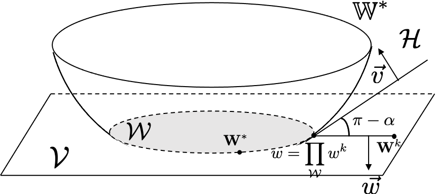
To this end, we propose a geometric condition. In particular, we assume that the target set 𝕎⋆\mathbb{W}^{\star} intersects with the set of achievable value vectors 𝒱={𝐕1π​(s1)|any policy π}\mathcal{V}=\{{\mathbf{V}}^{\pi}_{1}(s_{1})|\ \text{any policy $\pi$}\} nonsingularly—Figure 1 illustrates this concept. Formally, denote the set of achievable returns within the target set as 𝒲=𝒱∩𝕎⋆\mathcal{W}=\mathcal{V}\cap\mathbb{W}^{\star} and ∂𝒲=∂𝒱∩∂𝕎⋆\partial\mathcal{W}=\partial\mathcal{V}\cap\partial\mathbb{W}^{\star} as the intersection of the boundaries of 𝕎⋆\mathbb{W}^{\star} and the achievable value vector set 𝒱\mathcal{V}. Then, Assumption 5 describes nonsingular intersection.

Assumption 5.

If ∂𝒲\partial\mathcal{W} is not empty, then for each vector 𝐖∈∂𝒲\mathbf{W}\in\partial\mathcal{W}, denote the maximum angle α∈[0,π]\alpha\in[0,\pi] between the support vectors a→\vec{a} of 𝕎⋆\mathbb{W}^{\star} at 𝐖\mathbf{W} and the support vectors b→\vec{b} of 𝒱\mathcal{V} at 𝐖\mathbf{W} as

α(𝐖):=min{∠(a→,b→)|a→,b→are supportvectors of sets𝕎⋆and𝒱at𝐖}.\displaystyle\alpha(\mathbf{W}):=\min\{\angle(\vec{a},\vec{b})\ |\ \vec{a},\vec{b}\ \text{are support}\text{vectors of sets}\ \mathbb{W}^{\star}\ \text{and}\ \mathcal{V}\ \text{at}\ \mathbf{W}\}.

We assume there exists a constant αmax∈[π/2,π)\alpha_{\max}\in[\pi/2,\pi) such that maxw∈∂𝒲⁡α⁡(w)<αmax\max_{w\in\partial\mathcal{W}}\alpha(w)<\alpha_{\max}. With this upper bound on α\alpha, we denote γmin=sin⁡(π−αmax)>0\gamma_{\min}=\sin(\pi-\alpha_{\max})>0.

Refer to caption
Figure 1: The target set intersects with the achievable return vectors nonsingularly. The angle α⁡(∏𝒲𝐖k)\alpha(\prod_{\mathcal{W}}\mathbf{W}^{k}) is upper bounded.

Assumption 5 excludes the case where the sets 𝒱\mathcal{V} and 𝕎⋆\mathbb{W}^{\star} intersect tangentially (i.e., share the same supporting hyperplane) resulting in α=π\alpha=\pi. The necessity of such a geometric assumption is discussed in Appendix E.1. At a high level, Assumption 5 is a geometric analog of the previously noted strict interiority condition that excludes a singular intersection of the constraint functions gig_{i}. Our assumption provides a way to lower-bound the distance to the target set 𝕎⋆\mathbb{W}^{\star} by the distance to the actual constraint set 𝒲=𝒱∩𝕎⋆\mathcal{W}=\mathcal{V}\cap\mathbb{W}^{\star}, and thus prevent an algorithm from trading off too much constraint violation in exchange for a lower cost value g⁡(𝐕k)g(\mathbf{V}^{k}).

To minimize cost and avoid constraint violation simultaneously we need a “double” version of dual variable update. This idea is formalized in Double-Dual-Update below:

𝝋k+1\displaystyle\bm{\varphi}^{k+1} =Π𝔹d​{𝝋k+ηk​(𝐕^k−arg​max𝐱∈W⋆​𝝋k⋅𝐱)},\displaystyle=\Pi_{\mathbb{B}^{d}}\bigl\{\bm{\varphi}^{k}+\eta^{k}\bigl(\mathbf{\hat{V}}^{k}-\underset{\mathbf{x}\in W^{\star}}{\mathrm{arg}\max}\ \bm{\varphi}^{k}\cdot\mathbf{x}\bigr)\bigr\},
ϕk+1\displaystyle\bm{\phi}^{k+1} =Π𝔹d​{ϕk+ηk​(𝐕^k−∂g∗​(ϕk))},\displaystyle=\Pi_{\mathbb{B}^{d}}\bigl\{\bm{\phi}^{k}+\eta^{k}\bigl(\mathbf{\hat{V}}^{k}-\partial g^{*}(\bm{\phi}^{k})\bigr)\bigr\},
𝜽k+1\displaystyle\bm{\theta}^{k+1} =ρ​𝝋k+1+ϕk+1\displaystyle=\rho\bm{\varphi}^{k+1}+\bm{\phi}^{k+1} (Double-Dual-Update)

where Π𝔹d\Pi_{\mathbb{B}^{d}} denotes projection onto the dd-dimensional unit Euclidean ball and ∂g∗​(𝝋k)\partial g^{*}\bigl(\bm{\varphi}^{k}\bigr) is a subgradient vector of g∗g^{*} at 𝝋k\bm{\varphi}^{k} (not a set).

Algorithms Regret Constraint Violation Nonlinear Cost and Constraints Computionally Efficient
OptCMDP-bonus Efroni et al. 2020 𝒪~​(H4​S2​A​K)\mathcal{\tilde{O}}\left(\sqrt{H^{4}S^{2}AK}\right) 𝒪~​(d​H4​S2​A​K)\mathcal{\tilde{O}}\left(\sqrt{dH^{4}S^{2}AK}\right) ✓
Brantley et al. 2020 𝒪~​(H3​S2​A​K)\mathcal{\tilde{O}}\left(\sqrt{H^{3}S^{2}AK}\right) 𝒪~​(d3​H3​S2​A​K)\mathcal{\tilde{O}}\left(\sqrt{d^{3}H^{3}S^{2}AK}\right) ✓
OptPD-CMDP Efroni et al. 2020 𝒪~​((S2​A+d2)​H4​K)\mathcal{\tilde{O}}\left(\sqrt{(S^{2}A+d^{2})H^{4}K}\right) 𝒪~​((S2​A​d2+d3)​H4​K)\mathcal{\tilde{O}}\left(\sqrt{(S^{2}Ad^{2}+d^{3})H^{4}K}\right) ✓
OPDOP Ding et al. 2020 𝒪~​(H5​S4​A2​K)\mathcal{\tilde{O}}\left(\sqrt{H^{5}S^{4}A^{2}K}\right) 𝒪~​(H5​S4​A2​K)\mathcal{\tilde{O}}\left(\sqrt{H^{5}S^{4}A^{2}K}\right) ✓
UCPD Qiu et al. 2020 𝒪~​(H5​S2​A​K)\mathcal{\tilde{O}}\left(\sqrt{H^{5}S^{2}AK}\right) 𝒪~​(H5​S2​A​K)\mathcal{\tilde{O}}\left(\sqrt{H^{5}S^{2}AK}\right) ✓
This Paper 𝒪~​(min⁡{d,S}​d​H3​S​A​K)\mathcal{\tilde{O}}\left(\sqrt{\min\{d,S\}dH^{3}SAK}\right) 𝒪~​(min⁡{d,S}​d​H3​S​A​K)\mathcal{\tilde{O}}\left(\sqrt{\min\{d,S\}dH^{3}SAK}\right) ✓ ✓
Table 2: Comparison with constrained MDP literature.

Here comes our theoretical guarantee for both constraint violation and regret.

Theorem 5.

Following MOMA with VI-Bernstein (Algorithm 3) for Planning and Double-Dual-Update for Dual-Update, if 𝕎⋆\mathbb{W}^{\star} is approachable and μ⋆\mu^{\star} is a policy s.t. 𝐕1μ⋆​(s1)∈𝕎⋆\mathbf{V}^{\mu^{\star}}_{1}(s_{1})\in\mathbb{W}^{\star}, with probability 1−p1-p we can bound the constraint violation and the regret respectively as follows:

dist⁡(𝐖K,W⋆)\displaystyle\mathrm{dist}(\mathbf{W}^{K},W^{\star}) ≤𝒪⁡(min⁡{d,S}​d​H3​S​A​ι/K),\displaystyle\leq\mathcal{O}\bigl(\sqrt{\min\{d,S\}dH^{3}SA\iota/K}\bigr),
g⁡(𝐖K)−g⁡(𝐕1μ⋆​(s1))\displaystyle g(\mathbf{W}^{K})-g(\mathbf{V}^{\mu^{\star}}_{1}(s_{1})) ≤𝒪⁡(ρ​min⁡{d,S}​d​H3​S​A​ι/K),\displaystyle\leq\mathcal{O}\bigl(\rho\sqrt{\min\{d,S\}dH^{3}SA\iota/K}\bigr),

where ι=log⁡(S​A​K​H/p)\iota=\log\left(SAKH/p\right), ρ=2/γmin\rho=2/\gamma_{\min}.

Known results on constrained MDP problems do not share a common setup and hence make a precise comparison tricky. In short, our result aims to provide a computationally efficient algorithm for non-linear constraints (target set) and a convex cost function (see Table 2). Please see Appendix  C for a more detailed discussion of the subtleties among different constrained MDP setups, and some minor modifications needed to unify the exposition. With the existing results, our result is significant in the following aspects:

  • •

    First, our algorithm is the most general in terms of being able to handle non-linearity in the cost and constraints. The constrained MDP setting we study in Section 6.1 is a direct generalization of (Agrawal and Devanur 2014), and is closest to (Brantley et al. 2020). While our constraint assumption is equivalent to the one in (Brantley et al. 2020), our cost functions are more general. The domain of Brantley et al. 2020’s cost function is scalars, while that of ours is vectors.

  • •

    Furthermore, our proposed algorithm is computationally efficient because we do not require solving a large-scale convex optimization sub-problem with the number of variables and constraints scaling as 𝒪⁡(S​A​H)\mathcal{O}(SAH) per iteration (see Table 2). Indeed, our algorithms only comprise planning and model update procedures with a total of 𝒪⁡(S2​A​H)\mathcal{O}(S^{2}AH) basic algebraic updates in each episode, along with a dual space optimization procedure whose computational complexity is free of SS, AA and HH.

  • •

    Our bounds on regret and constraint violation are also the sharpest with respect to their dependence on the parameters SS, AA, and KK.

7 Conclusion and Future Work

In this paper, we formulate online learning in vector-valued Markov games via the lens of approaching a fixed convex target set within which the vector-valued objective should lie. We provide efficient model-based algorithms as instances of a generic meta-algorithm. Two key ideas contribute to our algorithmic design: (i) reduction of the vector-valued Markov game to a scalar-valued one, where the scalarization is iteratively updated; and (ii) exploration of the environment strategically. For vector-valued MDPs, our algorithms, after some modifications, achieve a tight rate in approaching the target set (in terms of S,A,H,KS,A,H,K), while simultaneously minimizing a convex cost function. Moreover, when the given target set is non-approachable, our algorithms automatically adapt to the degree of non-approachability.

Several problems are left open. Currently, there is still a d\sqrt{d} gap (dd is the dimensionality of the vector-valued cost) between our upper bound and the lower bound. How to close this gap to achieve the minimax rate remains unknown. The challenge in providing a tighter lower bound is that estimating a discrete distribution under the L2L^{2} distance does not get harder as the dimensionality increases. Since we use the Euclidean distance to measure the performance of our algorithms, we cannot get stronger dependence on dd. Lower bounds such as the one in (Jin et al. 2020) use a multiple hypothesis testing approach successfully because they work with an L1L^{1} loss, whereas we study the standard Euclidean loss. A second question is that our result in Section 6.1 has somewhat worse dependence on dd and ρ\rho compared to previous results. We leave improving the dimension dependency as a future direction.

Another future direction that is worth pursuing is that of redefining the notion of regret and error. Our work measures approachability error using the Euclidean distance. In practice, this choice may not be the only useful measure. Can we develop provably efficient algorithms under other geometries and measures of approachability? Answering this question might help exploit the geometry of the target set better, and potentially lead to tighter complexity analyses.

References

  • Abernethy et al. (2011) Jacob Abernethy, Peter L Bartlett, and Elad Hazan. Blackwell approachability and no-regret learning are equivalent. In Proceedings of the 24th Annual Conference on Learning Theory, pages 27–46, 2011.
  • Agrawal and Devanur (2014) Shipra Agrawal and Nikhil R Devanur. Bandits with concave rewards and convex knapsacks. In Proceedings of the fifteenth ACM conference on Economics and computation, pages 989–1006, 2014.
  • Azar et al. (2017) Mohammad Gheshlaghi Azar, Ian Osband, and Rémi Munos. Minimax regret bounds for reinforcement learning. In Proceedings of the 34th International Conference on Machine Learning-Volume 70, pages 263–272. JMLR. org, 2017.
  • Badanidiyuru et al. (2013) Ashwinkumar Badanidiyuru, Robert Kleinberg, and Aleksandrs Slivkins. Bandits with knapsacks. In 2013 IEEE 54th Annual Symposium on Foundations of Computer Science, pages 207–216. IEEE, 2013.
  • Bai and Jin (2020) Yu Bai and Chi Jin. Provable self-play algorithms for competitive reinforcement learning. arXiv preprint arXiv:2002.04017, 2020.
  • Bai et al. (2020) Yu Bai, Chi Jin, and Tiancheng Yu. Near-optimal reinforcement learning with self-play. arXiv preprint arXiv:2006.12007, 2020.
  • Blackwell (1956) David Blackwell. An analog of the minimax theorem for vector payoffs. Pacific Journal of Mathematics, 6(1):1–8, 1956.
  • Brafman and Tennenholtz (2002) Ronen I Brafman and Moshe Tennenholtz. R-max-a general polynomial time algorithm for near-optimal reinforcement learning. Journal of Machine Learning Research, 3(Oct):213–231, 2002.
  • Brantley et al. (2020) Kianté Brantley, Miroslav Dudik, Thodoris Lykouris, Sobhan Miryoosefi, Max Simchowitz, Aleksandrs Slivkins, and Wen Sun. Constrained episodic reinforcement learning in concave-convex and knapsack settings. arXiv preprint arXiv:2006.05051, 2020.
  • Chen et al. (2020) Xiaoyu Chen, Jiachen Hu, Lihong Li, and Liwei Wang. Efficient reinforcement learning in factored mdps with application to constrained rl. arXiv preprint arXiv:2008.13319, 2020.
  • Cheung et al. (2019) Wang Chi Cheung, David Simchi-Levi, and Ruihao Zhu. Non-stationary reinforcement learning: The blessing of (more) optimism. Available at SSRN 3397818, 2019.
  • Ding et al. (2020) Dongsheng Ding, Xiaohan Wei, Zhuoran Yang, Zhaoran Wang, and Mihailo R Jovanović. Provably efficient safe exploration via primal-dual policy optimization. arXiv preprint arXiv:2003.00534, 2020.
  • Domingues et al. (2020) Omar Darwiche Domingues, Pierre Ménard, Emilie Kaufmann, and Michal Valko. Episodic reinforcement learning in finite mdps: Minimax lower bounds revisited. arXiv preprint arXiv:2010.03531, 2020.
  • Efroni et al. (2020) Yonathan Efroni, Shie Mannor, and Matteo Pirotta. Exploration-exploitation in constrained mdps. arXiv preprint arXiv:2003.02189, 2020.
  • Jenatton et al. (2016) Rodolphe Jenatton, Jim Huang, and Cédric Archambeau. Adaptive algorithms for online convex optimization with long-term constraints. In International Conference on Machine Learning, pages 402–411. PMLR, 2016.
  • Jin et al. (2018) Chi Jin, Zeyuan Allen-Zhu, Sebastien Bubeck, and Michael I Jordan. Is Q-learning provably efficient? In Advances in Neural Information Processing Systems, pages 4863–4873, 2018.
  • Jin et al. (2020) Chi Jin, Akshay Krishnamurthy, Max Simchowitz, and Tiancheng Yu. Reward-free exploration for reinforcement learning. arXiv preprint arXiv:2002.02794, 2020.
  • Littman (1994) Michael L Littman. Markov games as a framework for multi-agent reinforcement learning. In Machine learning proceedings 1994, pages 157–163. Elsevier, 1994.
  • Liu et al. (2020) Qinghua Liu, Tiancheng Yu, Yu Bai, and Chi Jin. A sharp analysis of model-based reinforcement learning with self-play. arXiv preprint arXiv:2010.01604, 2020.
  • Mannor et al. (2014) Shie Mannor, Vianney Perchet, and Gilles Stoltz. Approachability in unknown games: Online learning meets multi-objective optimization. In Conference on Learning Theory, pages 339–355, 2014.
  • Maurer and Pontil (2009) Andreas Maurer and Massimiliano Pontil. Empirical bernstein bounds and sample variance penalization. arXiv preprint arXiv:0907.3740, 2009.
  • Neumann (1928) J v Neumann. Zur theorie der gesellschaftsspiele. Mathematische annalen, 100(1):295–320, 1928.
  • Osband and Van Roy (2014) Ian Osband and Benjamin Van Roy. Near-optimal reinforcement learning in factored mdps. Advances in Neural Information Processing Systems, 27:604–612, 2014.
  • Qiu et al. (2020) Shuang Qiu, Xiaohan Wei, Zhuoran Yang, Jieping Ye, and Zhaoran Wang. Upper confidence primal-dual reinforcement learning for cmdp with adversarial loss. Advances in Neural Information Processing Systems, 33, 2020.
  • Rockafellar (1970) R Tyrrell Rockafellar. Convex analysis. Number 28. Princeton university press, 1970.
  • Shapley (1953) Lloyd S Shapley. Stochastic games. Proceedings of the national academy of sciences, 39(10):1095–1100, 1953.
  • Shimkin (2016) Nahum Shimkin. An online convex optimization approach to blackwell’s approachability. The Journal of Machine Learning Research, 17(1):4434–4456, 2016.
  • Singh et al. (2020) Rahul Singh, Abhishek Gupta, and Ness B Shroff. Learning in markov decision processes under constraints. arXiv preprint arXiv:2002.12435, 2020.
  • Tian et al. (2020a) Yi Tian, Jian Qian, and Suvrit Sra. Towards minimax optimal reinforcement learning in factored markov decision processes. Advances in Neural Information Processing Systems, 33, 2020a.
  • Tian et al. (2020b) Yi Tian, Yuanhao Wang, Tiancheng Yu, and Suvrit Sra. Provably efficient online agnostic learning in markov games. arXiv preprint arXiv:2010.15020, 2020b.
  • Wu et al. (2020) Jingfeng Wu, Vladimir Braverman, and Lin F Yang. Accommodating picky customers: Regret bound and exploration complexity for multi-objective reinforcement learning. arXiv preprint arXiv:2011.13034, 2020.
  • Xie et al. (2020) Qiaomin Xie, Yudong Chen, Zhaoran Wang, and Zhuoran Yang. Learning Zero-Sum Simultaneous-Move Markov Games Using Function Approximation and Correlated Equilibrium. arXiv preprint arXiv:2002.07066, 2020.
  • Yuan and Lamperski (2018) Jianjun Yuan and Andrew Lamperski. Online convex optimization for cumulative constraints. In Advances in Neural Information Processing Systems, pages 6137–6146, 2018.

Appendix A Proofs for Section 3

In this section, we give detailed proofs needed in Section 3.

Beginning with a recapitulation of the notaions, We denote VkV^{k}, QkQ^{k}, πk\pi^{k}, μk\mu^{k}, νk\nu^{k} and θk\theta^{k} for values, policies and dual vectors at the beginning of the kk-th episode, In particular, Qhk​(s,a,b)=θk⋅Qhμk,νk​(s,a,b).Q^{k}_{h}(s,a,b)=\theta^{k}\cdot\ Q^{\mu_{k},\nu_{k}}_{h}(s,a,b).

𝐕^k\hat{\mathbf{V}}^{k} is the cumulative reward in the kk-th episode . In particular, Nhk​(s,a,b)N_{h}^{k}(s,a,b) is the number we have visited the state-action tuple (s,a,b)(s,a,b) at the hh-th step before the kk-th episode. Nhk​(s,a,b,s′)N_{h}^{k}(s,a,b,s^{\prime}) is defined by the same token. Using this notation, we can further define the empirical transition and exploration bonus by ℙ^hk​(s′|s,a,b):=Nhk​(s,a,b,s′)/Nhk​(s,a,b)\widehat{\mathbb{P}}^{k}_{h}(s^{\prime}|s,a,b):=N^{k}_{h}(s,a,b,s^{\prime})/N^{k}_{h}(s,a,b) and βhk​(s,a,b):=C​min⁡{d,S}​d​ι​H2/Nhk​(s,a,b)\beta_{h}^{k}(s,a,b):=C\sqrt{\min\{d,S\}d\iota H^{2}/N_{h}^{k}(s,a,b)}.

We first give a uniform convergence guarantee, which will also be used later. The first simple lemma is from Liu et al. 2020.

Lemma 6.

Let 𝕏,𝐘,𝐙∈ℝA×B\mathbb{X},\mathbf{Y},\mathbf{Z}\in\mathbb{R}^{A\times B} and Δd\Delta_{d} be the dd-dimensional simplex. Suppose |𝕏−𝐘|≤𝐙\left|\mathbb{X}-\mathbf{Y}\right|\leq\mathbf{Z}, where the inequality is entry-wise. Then

|maxμ∈△A⁡minν∈△B​μ⊤​𝕏​ν−maxμ∈△A⁡minν∈△B​μ⊤​𝐘​ν|≤maxi,j⁡𝐙i​j.\left|\max_{\mu\in\triangle_{A}}\min_{\nu\in\triangle_{B}}\mu^{\top}\mathbb{X}\nu-\max_{\mu\in\triangle_{A}}\min_{\nu\in\triangle_{B}}\mu^{\top}\mathbf{Y}\nu\right|\leq\max_{i,j}\mathbf{Z}_{ij}. (A.1)

We also need to following lemma to characterize the dependence of V⋆​(𝜽k,⋅)V^{\star}(\bm{\theta}^{k},\cdot) on 𝜽k\bm{\theta}^{k} to apply the covering argument.

Lemma 7 (Lipschitz property of V⋆V^{\star}).

For any s∈𝒮s\in\mathcal{S},

|Vh⋆​(𝜽,s)−Vh⋆​(𝜽′,s)|≤d​(H−h+1)​‖𝜽−𝜽′‖2\left|V^{\star}_{h}(\bm{\theta},s)-V^{\star}_{h}(\bm{\theta}^{\prime},s)\right|\leq\sqrt{d}(H-h+1)\left\|\bm{\theta}-\bm{\theta}^{\prime}\right\|_{2}
Proof.

By Cauchy-Schwarz, |Vh⋆​(𝜽,s)|≤d​(H−h+1)|V^{\star}_{h}(\bm{\theta},s)|\leq\sqrt{d}(H-h+1). The rest of proof follows by induction via Bellman equation and Lemma 6. ∎

Equipped with this Lipschitz property, we are ready to prove a uniform concentration result. Notice 𝔹d\mathbb{B}^{d} is the dd-dimensional unit Euclidean ball centered at 00.

Lemma 8 (Uniform Concentration of V⋆​(𝜽,⋅)V^{\star}(\bm{\theta},\cdot)).

Consider value function class

𝒱h+1={V:𝒮→ℝ∣V(⋅)=Vh+1⋆(𝜽,⋅)for all𝜽∈𝔹m}.\mathcal{V}_{h+1}={\left\{V:\mathcal{S}\to\mathbb{R}~\mid~V(\cdot)=V_{h+1}^{\star}\left(\bm{\theta},\cdot\right)~\textrm{for all}~\bm{\theta}\in\mathbb{B}^{m}\right\}}.

There exists an absolute constant cc, with probability at least 1−p1-p, for all (s,a,b,k,h)(s,a,b,k,h) and all V∈𝒱h+1V\in\mathcal{V}_{h+1} we have:

|[(ℙ^hk−ℙh)​V]​(s,a,b)|≤c​min⁡{d,S}​d​H2​ιNhk​(s,a).|{[(\hat{\mathbb{P}}^{k}_{h}-\mathbb{P}_{h})V](s,a,b)}|\leq c\sqrt{\frac{\min\{d,S\}dH^{2}\iota}{N_{h}^{k}(s,a)}}.

where ι=log⁡(m​S​A​B​K​H/p)\iota=\log(mSABKH/p) is a logarithmic factor.

Proof.

Let 𝒟ϵ\mathcal{D}_{\epsilon} be an ϵ\epsilon-covering of 𝔹d\mathbb{B}^{d} in the ℒ2\mathcal{L}^{2} norm, i.e., for any 𝜽∈𝔹d\bm{\theta}\in\mathbb{B}^{d} there exists 𝜽^∈𝒟ϵ\hat{\bm{\theta}}\in\mathcal{D}_{\epsilon} such that ‖𝜽−𝜽^‖2≤ϵ\left\|\bm{\theta}-\hat{\bm{\theta}}\right\|_{2}\leq\epsilon. For each 𝜽^∈𝒟ϵ\hat{\bm{\theta}}\in\mathcal{D}_{\epsilon}, we can define the corresponding value function Vh+1⋆​(𝜽^,⋅)V_{h+1}^{\star}\left(\hat{\bm{\theta}},\cdot\right). In this way, by Lemma 7, we can generate a set 𝒱ϵ\mathcal{V}_{\epsilon} which is an H​ϵH\epsilon-covering of 𝒱h+1\mathcal{V}_{h+1} in infinity norm, i.e., for any V∈𝒱h+1V\in\mathcal{V}_{h+1} there exists V^∈𝒱ϵ\hat{V}\in\mathcal{V}_{\epsilon} such that for any s∈𝒮s\in\mathcal{S}, |V⁡(s)−V^​(s)|≤H​ϵ|V(s)-\hat{V}(s)|\leq H\epsilon .

Since |𝒟ϵ|≤(1/ϵ)d|\mathcal{D}_{\epsilon}|\leq(1/\epsilon)^{d}, we also have |𝒱ϵ|≤(1/ϵ)d|\mathcal{V}_{\epsilon}|\leq(1/\epsilon)^{d}. Since |Vh⋆​(𝜽,s)|≤d​(H−h+1)|V^{\star}_{h}(\bm{\theta},s)|\leq\sqrt{d}(H-h+1), by Hoeffding inequality and taking union bound, with probability at least 1−p1-p,

|supV^∈𝒱ϵ[(ℙ^hk−ℙh)​V]​(s,a,b)|≤𝒪⁡(d2​H2​ι′Nhk​(s,a)).\displaystyle|{\sup_{\hat{V}\in\mathcal{V}_{\epsilon}}[(\hat{\mathbb{P}}^{k}_{h}-\mathbb{P}_{h})V](s,a,b)}|\leq\mathcal{O}\left(\sqrt{\frac{d^{2}H^{2}\iota^{\prime}}{N_{h}^{k}(s,a)}}\right).

where ι′=ι+log⁡1/ϵ\iota^{\prime}=\iota+\log 1/\epsilon.

At the same time, for any V∈𝒱h+1V\in\mathcal{V}_{h+1}, there exists V^∈𝒱ϵ\hat{V}\in\mathcal{V}_{\epsilon} such that sups|V⁡(s)−V^​(s)|≤d​H​ϵ\sup_{s}|V(s)-\hat{V}(s)|\leq\sqrt{d}H\epsilon. Therefore,

|[(ℙ^hk−ℙh)​V]​(s,a,b)|≤|[(ℙ^hk−ℙh)​V^]​(s,a,b)|+d​H​ϵ.|{[(\hat{\mathbb{P}}^{k}_{h}-\mathbb{P}_{h})V](s,a,b)}|\leq|{[(\hat{\mathbb{P}}^{k}_{h}-\mathbb{P}_{h})\hat{V}](s,a,b)}|+\sqrt{d}H\epsilon.

Taking ϵ=d​ι/Nhk​(s,a)\epsilon=d\iota/N_{h}^{k}(s,a) proves

|[(ℙ^hk−ℙh)​V]​(s,a,b)|≤c​d2​H2​ιNhk​(s,a).|{[(\hat{\mathbb{P}}^{k}_{h}-\mathbb{P}_{h})V](s,a,b)}|\leq c\sqrt{\frac{d^{2}H^{2}\iota}{N_{h}^{k}(s,a)}}.

Similarly we also have (for example see Lemma 12 in Bai and Jin 2020)

|[(ℙ^hk−ℙh)​V]​(s,a,b)|≤c​d​S​H2​ιNhk​(s,a),|{[(\hat{\mathbb{P}}^{k}_{h}-\mathbb{P}_{h})V](s,a,b)}|\leq c\sqrt{\frac{dSH^{2}\iota}{N_{h}^{k}(s,a)}},

∎

which completes the proof.

Using the concentration result, we can prove the "lower confidence bounds" are indeed lower bounds with high probability. To do this, we need to introduce a little more notation.

Similar to Vh⋆V^{\star}_{h}, we can also define Q⋆Q^{\star}. By Bellman equation we have

Qh⋆​(𝜽,s,a,b)=[𝜽⋅𝐫h+ℙh​Vh+1⋆​(𝜽,⋅)]​(s,a,b).Q^{\star}_{h}(\bm{\theta},s,a,b)=[\bm{\theta}\cdot\mathbf{r}_{h}+\mathbb{P}_{h}V^{\star}_{h+1}(\bm{\theta},\cdot)](s,a,b).
Lemma 9 (Upper confidence bound).

With probability 1−p1-p, for all h,s,a,bh,s,a,b and k∈[K]k\in[K], we have

Qhk​(s,a,b)≤Qh⋆​(𝜽k,s,a,b),Vhk​(s)≤Vh⋆​(𝜽k,s).Q^{k}_{h}(s,a,b)\leq Q^{\star}_{h}(\bm{\theta}^{k},s,a,b),\,\,\,\,V^{k}_{h}(s)\leq V^{\star}_{h}(\bm{\theta}^{k},s). (A.2)
Proof.

Again, the proof is by backward induction. Suppose the bounds hold for the Q-values in the (h+1)(h+1)-th step, we now establish the bounds for the values in the (h+1)(h+1)-th step and Q-values in the hh-step. Consider a fixed state ss,

Vh+1k​(s)\displaystyle V^{k}_{h+1}(s) =𝔻πhk​Qh+1k​(s)\displaystyle=\mathbb{D}_{\pi^{k}_{h}}Q^{k}_{h+1}(s) (A.3)
=minυ⁡𝔻μh+1k×υ​Qh+1k​(s)\displaystyle=\min_{\upsilon}\mathbb{D}_{\mu^{k}_{h+1}\times\upsilon}Q^{k}_{h+1}(s)
≤minυ⁡𝔻μh+1k×υ​Qh⋆​(𝜽k,⋅,⋅,⋅)​(s)\displaystyle\leq\min_{\upsilon}\mathbb{D}_{\mu^{k}_{h+1}\times\upsilon}Q^{\star}_{h}(\bm{\theta}^{k},\cdot,\cdot,\cdot)(s)
≤Vh⋆​(𝜽k,s).\displaystyle\leq V^{\star}_{h}(\bm{\theta}^{k},s).

Now consider a fixed triple (s,a,b)(s,a,b) at hh-th step. We have

Qhk​(s,a,b)−Qh⋆​(𝜽k,s,a,b)=\displaystyle Q^{k}_{h}(s,a,b)-Q^{\star}_{h}(\bm{\theta}^{k},s,a,b)= (ℙ^hk​Vh+1k−ℙh​Vh+1⋆​(𝜽k,⋅)−βhk)​(s,a,b)\displaystyle(\widehat{\mathbb{P}}_{h}^{k}V^{k}_{h+1}-\mathbb{P}_{h}V^{\star}_{h+1}(\bm{\theta}^{k},\cdot)-\beta_{h}^{k})(s,a,b) (A.4)
≤(i)\displaystyle\overset{\left(i\right)}{\leq} [(ℙ^hk−ℙh)​Vh+1⋆​(𝜽k,⋅)]​(s,a,b)−βhk​(s,a)\displaystyle[(\widehat{\mathbb{P}}_{h}^{k}-\mathbb{P}_{h})V^{\star}_{h+1}(\bm{\theta}^{k},\cdot)](s,a,b)-\beta_{h}^{k}(s,a)
≤(i​i)\displaystyle\overset{\left(ii\right)}{\leq} 0.\displaystyle 0.

where (i)(i) is by induction hypothesis and (i​i)(ii) is by Lemma 8 and the definition of β\beta. ∎

A handy decomposition will help us simplify the target we want to bound in Theorem 1 and Theorem 2. To simplify the notation, when there are no confusion, we use the shorthand Vμk,νkV^{\mu^{k},\nu^{k}} and Qμk,νkQ^{\mu^{k},\nu^{k}} for 𝜽k⋅𝐕μk,νk\bm{\theta}^{k}\cdot\mathbf{V}^{\mu^{k},\nu^{k}} and 𝜽k⋅𝐐μk,νk\bm{\theta}^{k}\cdot\mathbf{Q}^{\mu^{k},\nu^{k}}.

Lemma 10 (Regret decomposition).

The "regret" [V1μk,νk−V1k]​(s1k)[V_{1}^{\mu^{k},\nu^{k}}-V_{1}^{k}](s_{1}^{k}) can be decompsed into

[V1μk,νk−V1k]​(s1k)≤∑h=1H(βhk+ξhk+ζhk)[V_{1}^{\mu^{k},\nu^{k}}-V_{1}^{k}](s_{1}^{k})\leq\sum_{h=1}^{H}{\left(\beta_{h}^{k}+\xi_{h}^{k}+\zeta_{h}^{k}\right)}

where

ξhk:=\displaystyle\xi_{h}^{k}:= (𝔻μk×νk​Qhμk,νk−𝔻μk×νk​Qhk)​(shk)−(Qhμk,νk−Qhk)​(shk,ahk,bhk)∈[−4​d​H,4​d​H],\displaystyle\left(\mathbb{D}_{\mu^{k}\times\nu^{k}}Q_{h}^{\mu^{k},\nu^{k}}-\mathbb{D}_{\mu^{k}\times\nu^{k}}Q_{h}^{k}\right)(s_{h}^{k})-\left(Q_{h}^{\mu^{k},\nu^{k}}-Q_{h}^{k}\right)\left(s_{h}^{k},a_{h}^{k},b_{h}^{k}\right)\in\left[-4\sqrt{d}H,4\sqrt{d}H\right],
ζhk:=\displaystyle\zeta_{h}^{k}:= ℙh​(Vh+1μk,νk−Vh+1k)​(shk,ahk,bhk)−(Vh+1μk,νk−Vh+1k)​(shk)∈[−4​d​H,4​d​H]\displaystyle\mathbb{P}_{h}\left(V_{h+1}^{\mu^{k},\nu^{k}}-V_{h+1}^{k}\right)\left(s_{h}^{k},a_{h}^{k},b_{h}^{k}\right)-\left(V_{h+1}^{\mu^{k},\nu^{k}}-V_{h+1}^{k}\right)\left(s_{h}^{k}\right)\in\left[-4\sqrt{d}H,4\sqrt{d}H\right]

are martingale difference sequences adapted to ℱhk\mathcal{F}_{h}^{k}.

Proof.

We have

[Vhμk,νk−Vhk]​(shk)=\displaystyle[V_{h}^{\mu^{k},\nu^{k}}-V_{h}^{k}](s_{h}^{k})= (𝔻μk×νk​Qhμk,νk−𝔻πk​Qhk)​(shk)\displaystyle\left(\mathbb{D}_{\mu^{k}\times\nu^{k}}Q_{h}^{\mu^{k},\nu^{k}}-\mathbb{D}_{\pi^{k}}Q_{h}^{k}\right)(s_{h}^{k})
≤(i)\displaystyle\overset{\left(i\right)}{\leq} (𝔻μk×νk​Qhμk,νk−𝔻μk×νk​Qhk)​(shk)\displaystyle\left(\mathbb{D}_{\mu^{k}\times\nu^{k}}Q_{h}^{\mu^{k},\nu^{k}}-\mathbb{D}_{\mu^{k}\times\nu^{k}}Q_{h}^{k}\right)(s_{h}^{k})
=\displaystyle= (Qhμk,νk−Qhk)​(shk,ahk,bhk)+ξhk\displaystyle\left(Q_{h}^{\mu^{k},\nu^{k}}-Q_{h}^{k}\right)\left(s_{h}^{k},a_{h}^{k},b_{h}^{k}\right)+\xi_{h}^{k}
=\displaystyle= ℙh​(Vh+1μk,νk−Vh+1k)​(shk,ahk,bhk)+βhk+ξhk\displaystyle\mathbb{P}_{h}\left(V_{h+1}^{\mu^{k},\nu^{k}}-V_{h+1}^{k}\right)\left(s_{h}^{k},a_{h}^{k},b_{h}^{k}\right)+\beta_{h}^{k}+\xi_{h}^{k}
=\displaystyle= (Vh+1μk,νk−Vh+1k)​(sh+1k)+βhk+ξhk+ζhk.\displaystyle\left(V_{h+1}^{\mu^{k},\nu^{k}}-V_{h+1}^{k}\right)\left(s_{h+1}^{k}\right)+\beta_{h}^{k}+\xi_{h}^{k}+\zeta_{h}^{k}.

where (i)(i) is by the definition of Nash equilibirum.

Repete the recursion we have

[V1μk,νk−V1k]​(s1k)≤∑h=1H(βhk+ξhk+ζhk).[V_{1}^{\mu^{k},\nu^{k}}-V_{1}^{k}](s_{1}^{k})\leq\sum_{h=1}^{H}{\left(\beta_{h}^{k}+\xi_{h}^{k}+\zeta_{h}^{k}\right)}.

∎

The sum of the exploration bonus can be bounded easily.

Lemma 11 (Sum of bonus).
∑k=1K∑h=1Hβhk≤O⁡(min⁡{d,S}​d​H4​S​A​B​K​ι)\sum_{k=1}^{K}{\sum_{h=1}^{H}{\beta_{h}^{k}}}\leq O\left(\sqrt{\min\{d,S\}dH^{4}SABK\iota}\right)
Proof.

By definition of β\beta and pigeonhole principle,

∑k=1K∑h=1Hβhk≤\displaystyle\sum_{k=1}^{K}{\sum_{h=1}^{H}{\beta_{h}^{k}}}\leq ∑k=1K∑h=1HO⁡(min⁡{d,S}​d​H2​ιNhk​(shk,ahk,bhk))\displaystyle\sum_{k=1}^{K}{\sum_{h=1}^{H}{O\left(\sqrt{\frac{\min\{d,S\}dH^{2}\iota}{N_{h}^{k}\left(s_{h}^{k},a_{h}^{k},b_{h}^{k}\right)}}\right)}}
≤\displaystyle\leq O⁡(∑h=1H∑s,a,b∑t=1NhK​(s,a,b)min⁡{d,S}​d​H2​ιt)\displaystyle O\left(\sum_{h=1}^{H}{\sum_{s,a,b}{\sum_{t=1}^{N_{h}^{K}\left(s,a,b\right)}{\sqrt{\frac{\min\{d,S\}dH^{2}\iota}{t}}}}}\right)
≤\displaystyle\leq O⁡(∑h=1H∑s,a,bmin⁡{d,S}​d​H2​ι​NhK​(s,a,b))\displaystyle O\left(\sum_{h=1}^{H}{\sum_{s,a,b}{\sqrt{\min\{d,S\}dH^{2}\iota N_{h}^{K}\left(s,a,b\right)}}}\right)
≤\displaystyle\leq O⁡(min⁡{d,S}​d​H4​S​A​B​K​ι).\displaystyle O\left(\sqrt{\min\{d,S\}dH^{4}SABK\iota}\right).

∎

Now we are ready to prove Theorem 1 and Theorem 2.

Proof of Theorem 1.

The squared distance can be demcoposed by

dist​(𝐖k,W⋆)2=\displaystyle\mathrm{dist}\left(\mathbf{W}^{k},W^{\star}\right)^{2}= ∥𝐖k−ΠW∗​(𝐖k)∥22\displaystyle\lVert\mathbf{W}^{k}-\Pi_{W^{*}}\left(\mathbf{W}^{k}\right)\rVert_{2}^{2}
≤(i)\displaystyle\overset{\left(i\right)}{\leq} ∥𝐖k−ΠW⋆​(𝐖k−1)∥22\displaystyle\lVert\mathbf{W}^{k}-\Pi_{W^{\star}}\left(\mathbf{W}^{k-1}\right)\rVert_{2}^{2}
=\displaystyle= ∥k−1k​𝐖k−1+1k​𝐕^k−ΠW⋆​(𝐖k−1)∥22\displaystyle\lVert\frac{k-1}{k}\mathbf{W}^{k-1}+\frac{1}{k}\mathbf{\hat{V}}^{k}-\Pi_{W^{\star}}\left(\mathbf{W}^{k-1}\right)\rVert_{2}^{2}
=\displaystyle= (k−1k)2​dist​(𝐖k−1,W⋆)2+1k2​‖𝐕^k−ΠW⋆​(𝐖k−1)‖22⏟(A)\displaystyle\left(\frac{k-1}{k}\right)^{2}\mathrm{dist}\left(\mathbf{W}^{k-1},W^{\star}\right)^{2}+\frac{1}{k^{2}}\underset{\left(A\right)}{\underbrace{\left\|\mathbf{\hat{V}}^{k}-\Pi_{W^{\star}}\left(\mathbf{W}^{k-1}\right)\right\|_{2}^{2}}}
+2​(k−1)k2​(𝐖k−1−ΠW⋆​(𝐖k−1))⋅(𝐕^k−ΠW⋆​(𝐖k−1))⏟(B)\displaystyle+\frac{2\left(k-1\right)}{k^{2}}\underset{\left(B\right)}{\underbrace{\left(\mathbf{W}^{k-1}-\Pi_{W^{\star}}\left(\mathbf{W}^{k-1}\right)\right)\cdot\left(\mathbf{\hat{V}}^{k}-\Pi_{W^{\star}}\left(\mathbf{W}^{k-1}\right)\right)}}

where (i)(i) is by the definition of (Euclidean) projection.

By boundedness of distance, (A)=∥𝐕^k−ΠW⋆​(𝐖k−1)∥22≤d​H2(A)=\lVert\mathbf{\hat{V}}^{k}-\Pi_{W^{\star}}\left(\mathbf{W}^{k-1}\right)\rVert_{2}^{2}\leq dH^{2}.

To bound (B)(B), we notice if 𝐖k−1∈W⋆\mathbf{W}^{k-1}\in W^{\star}, dist⁡(𝐖k−1,W⋆)\mathrm{dist}\left(\mathbf{W}^{k-1},W^{\star}\right) and

(B)=0=dist⁡(𝐖k−1,W⋆)​𝜽k⋅(𝐕^k−ΠW⋆​(𝐖k−1))(B)=0=\mathrm{dist}\left(\mathbf{W}^{k-1},W^{\star}\right)\bm{\theta}^{k}\cdot\left(\mathbf{\hat{V}}^{k}-\Pi_{W^{\star}}\left(\mathbf{W}^{k-1}\right)\right)

for any 𝜽k\bm{\theta}^{k}. Otherwise,

(B)=\displaystyle(B)= (𝐖k−1−ΠW⋆​(𝐖k−1))⋅(𝐕^k−ΠW⋆​(𝐖k−1))\displaystyle\left(\mathbf{W}^{k-1}-\Pi_{W^{\star}}\left(\mathbf{W}^{k-1}\right)\right)\cdot\left(\mathbf{\hat{V}}^{k}-\Pi_{W^{\star}}\left(\mathbf{W}^{k-1}\right)\right)
=\displaystyle= dist⁡(𝐖k−1,W⋆)​𝜽k⋅(𝐕^k−ΠW⋆​(𝐖k−1))\displaystyle\mathrm{dist}\left(\mathbf{W}^{k-1},W^{\star}\right)\bm{\theta}^{k}\cdot\left(\mathbf{\hat{V}}^{k}-\Pi_{W^{\star}}\left(\mathbf{W}^{k-1}\right)\right)
≤(i)\displaystyle\overset{\left(i\right)}{\leq} dist⁡(𝐖k−1,W⋆)​(𝜽k⋅𝐕^k−V1⋆​(𝜽k,s1k))\displaystyle\mathrm{dist}\left(\mathbf{W}^{k-1},W^{\star}\right)\left(\bm{\theta}^{k}\cdot\mathbf{\hat{V}}^{k}-V_{1}^{\star}\left(\bm{\theta}^{k},s_{1}^{k}\right)\right)
≤(i​i)\displaystyle\overset{\left(ii\right)}{\leq} dist⁡(𝐖k−1,W⋆)​(𝜽k⋅𝐕^k−V1k​(s1k))\displaystyle\mathrm{dist}\left(\mathbf{W}^{k-1},W^{\star}\right)\left(\bm{\theta}^{k}\cdot\mathbf{\hat{V}}^{k}-V_{1}^{k}\left(s_{1}^{k}\right)\right)
=\displaystyle= dist⁡(𝐖k−1,W⋆)​[(V1μk,νk−V1k)​(s1k)+(𝜽k⋅𝐕^k−V1μk,νk​(s1k))]\displaystyle\mathrm{dist}\left(\mathbf{W}^{k-1},W^{\star}\right)\left[\left(V_{1}^{\mu^{k},\nu^{k}}-V_{1}^{k}\right)\left(s_{1}^{k}\right)+\left(\bm{\theta}^{k}\cdot\mathbf{\hat{V}}^{k}-V_{1}^{\mu^{k},\nu^{k}}\left(s_{1}^{k}\right)\right)\right]
≤(i​i​i)\displaystyle\overset{\left(iii\right)}{\leq} dist⁡(𝐖k−1,W⋆)​[∑h=1H(βhk+ξhk+ζhk)+(𝜽k⋅𝐕^k−V1μk,νk​(s1k))]\displaystyle\mathrm{dist}\left(\mathbf{W}^{k-1},W^{\star}\right)\left[\sum_{h=1}^{H}{\left(\beta_{h}^{k}+\xi_{h}^{k}+\zeta_{h}^{k}\right)}+\left(\bm{\theta}^{k}\cdot\mathbf{\hat{V}}^{k}-V_{1}^{\mu^{k},\nu^{k}}\left(s_{1}^{k}\right)\right)\right]

where (i)(i) is by Approachability (Assumption 3), (i​i)(ii) is by optimism (Lemma 9) and (i​i​i)(iii) is by regret decomposition (Lemma 10).

Putting everything together and repete the recursion we have

K​dist​(𝐖K,W∗)2≤d​H2+2​∑k=1Kk−1K​dist​(𝐖k−1,W⋆)​[∑h=1H(βhk+ξhk+ζhk)+(𝜽k⋅𝐕^k−V1μk,νk​(s1k))]K\mathrm{dist}\left(\mathbf{W}^{K},W^{*}\right)^{2}\leq dH^{2}+2\sum_{k=1}^{K}{\frac{k-1}{K}}\mathrm{dist}\left(\mathbf{W}^{k-1},W^{\star}\right)\left[\sum_{h=1}^{H}{\left(\beta_{h}^{k}+\xi_{h}^{k}+\zeta_{h}^{k}\right)}+\left(\bm{\theta}^{k}\cdot\mathbf{\hat{V}}^{k}-V_{1}^{\mu^{k},\nu^{k}}\left(s_{1}^{k}\right)\right)\right]

Now we can begin to prove the theorem by induction. Suppose

dist⁡(𝐖k,W⋆)≤c0​min⁡{d,S}​d​H4​S​A​B​ι/k.\mathrm{dist}\left(\mathbf{W}^{k},W^{\star}\right)\leq c_{0}\sqrt{\min\{d,S\}dH^{4}SAB\iota/k}.

for ∀k≤K−1\forall k\leq K-1, let’s prove the claim holds for k=Kk=K. We first consider the optimistic bonus.

∑k=1K∑h=1Hk−1K​dist​(𝐖k−1,W⋆)​βhk≤\displaystyle\sum_{k=1}^{K}{\sum_{h=1}^{H}{\frac{k-1}{K}\mathrm{dist}\left(\mathbf{W}^{k-1},W^{\star}\right)\beta_{h}^{k}}}\leq c0​min⁡{d,S}​d​H4​S​A​B​ι​∑k=1K∑h=1HkK​βhk\displaystyle c_{0}\sqrt{\min\{d,S\}dH^{4}SAB\iota}\sum_{k=1}^{K}{\sum_{h=1}^{H}{\frac{\sqrt{k}}{K}\beta_{h}^{k}}}
≤\displaystyle\leq c0​min⁡{d,S}​d​H4​S​A​B​ι/K​∑k=1K∑h=1Hβhk\displaystyle c_{0}\sqrt{\min\{d,S\}dH^{4}SAB\iota/K}\sum_{k=1}^{K}{\sum_{h=1}^{H}{\beta_{h}^{k}}}
≤(i)\displaystyle\overset{\left(i\right)}{\leq} c0​c1​min⁡{d,S}​d​H4​S​A​B​ι\displaystyle c_{0}c_{1}\min\{d,S\}dH^{4}SAB\iota

where (i)(i) is by Lemma 11 and c1c_{1} is the constant coefficient there.

The remaining terms are martingale difference sequence, so we only need to bound the variance.

∑k=1K∑h=1Hk−1K​dist​(𝐖k−1,W⋆)​ξhk​≤(i)\displaystyle\sum_{k=1}^{K}{\sum_{h=1}^{H}{\frac{k-1}{K}\mathrm{dist}\left(\mathbf{W}^{k-1},W^{\star}\right)\xi_{h}^{k}}}\overset{\left(i\right)}{\leq} c2​∑k=1K(k−1K)2​dist​(𝐖k−1,W⋆)2​d​H3​ι\displaystyle c_{2}\sqrt{\sum_{k=1}^{K}{\left(\frac{k-1}{K}\right)^{2}}\mathrm{dist}\left(\mathbf{W}^{k-1},W^{\star}\right)^{2}dH^{3}\iota}
≤\displaystyle\leq c2​c0​min⁡{d,S}​d2​H4​S​A​B​ι2​∑k=1Kk​H3K2\displaystyle c_{2}c_{0}\sqrt{\min\{d,S\}d^{2}H^{4}SAB\iota^{2}}\sqrt{\sum_{k=1}^{K}{\frac{kH^{3}}{K^{2}}}}
≤\displaystyle\leq c0​c1​min⁡{d,S}​d2​H7​S​A​B​ι2\displaystyle c_{0}c_{1}\sqrt{\min\{d,S\}d^{2}H^{7}SAB\iota^{2}}

where (i)(i) is by Azuma-Hoeffding. Similarly, ∑k=1K∑h=1Hk−1K​dist​(𝐖k−1,W⋆)​ζhk≤c2​c0​min⁡{d,S}​d2​H7​S​A​B​ι2\sum_{k=1}^{K}{\sum_{h=1}^{H}{\frac{k-1}{K}\mathrm{dist}\left(\mathbf{W}^{k-1},W^{\star}\right)\zeta_{h}^{k}}}\leq c_{2}c_{0}\sqrt{\min\{d,S\}d^{2}H^{7}SAB\iota^{2}}.

The last term can be handled similarly but we need to be more carefully because different coordinates of 𝐕^k\mathbf{\hat{V}}^{k} are correlated.

∑k=1Kk−1K​dist​(𝐖k−1,W⋆)​(𝜽k⋅𝐕^k−V1μk,νk​(s1k))≤\displaystyle\sum_{k=1}^{K}{\frac{k-1}{K}\mathrm{dist}\left(\mathbf{W}^{k-1},W^{\star}\right)\left(\bm{\theta}^{k}\cdot\mathbf{\hat{V}}^{k}-V_{1}^{\mu^{k},\nu^{k}}\left(s_{1}^{k}\right)\right)}\leq c2​∑j=1m∑k=1K(k−1K)2​dist​(𝐖k−1,W⋆)2​(𝜽jk)2​H2​ι\displaystyle c_{2}\sum_{j=1}^{m}{\sqrt{\sum_{k=1}^{K}{\left(\frac{k-1}{K}\right)^{2}}\mathrm{dist}\left(\mathbf{W}^{k-1},W^{\star}\right)^{2}\left(\bm{\theta}^{k}_{j}\right)^{2}H^{2}\iota}}
≤\displaystyle\leq c2​c0​min⁡{d,S}​d​H4​S​A​B​ι2​∑j=1m∑k=1K(𝜽jk)2​k​H2K2\displaystyle c_{2}c_{0}\sqrt{\min\{d,S\}dH^{4}SAB\iota^{2}}\sum_{j=1}^{m}{\sqrt{\sum_{k=1}^{K}{\left(\bm{\theta}^{k}_{j}\right)^{2}\frac{kH^{2}}{K^{2}}}}}
≤(i)\displaystyle\overset{\left(i\right)}{\leq} c2​c0​min⁡{d,S}​d​H4​S​A​B​ι2​m​∑j=1m∑k=1K(𝜽jk)2​k​H2K2\displaystyle c_{2}c_{0}\sqrt{\min\{d,S\}dH^{4}SAB\iota^{2}}\sqrt{m\sum_{j=1}^{m}{\sum_{k=1}^{K}{\left(\bm{\theta}^{k}_{j}\right)^{2}\frac{kH^{2}}{K^{2}}}}}
=\displaystyle= c2​c0​min⁡{d,S}​d2​H4​S​A​B​ι2​∑k=1Kk​H2K2\displaystyle c_{2}c_{0}\sqrt{\min\{d,S\}d^{2}H^{4}SAB\iota^{2}}\sqrt{\sum_{k=1}^{K}{\frac{kH^{2}}{K^{2}}}}
≤\displaystyle\leq c2​c0​min⁡{d,S}​d2​H6​S​A​B​ι2\displaystyle c_{2}c_{0}\sqrt{\min\{d,S\}d^{2}H^{6}SAB\iota^{2}}

where (i)(i) is by Cauchy-Schwarz.

After taking a union bound w.r.t. [K][K], to prove the claim for k=Kk=K, we only need to guarantee

d​H2+8​c0​max​{c1,c2}​min​{d,S}​d​H4​S​A​B​ι≤c02​min​{d,S}​d​H4​S​A​B​ιdH^{2}+8c_{0}\max\left\{c_{1},c_{2}\right\}\min\{d,S\}dH^{4}SAB\iota\leq c_{0}^{2}\min\{d,S\}dH^{4}SAB\iota

which is satisfied as long as c0≥max⁡{16​max⁡{c1,c2},2S​A​B​H2​ι}c_{0}\geq\max\left\{16\max\left\{c_{1},c_{2}\right\},\sqrt{\frac{2}{SABH^{2}\iota}}\right\}. ∎

We can prve Theorem 2 similarly.

Proof of Theorem 2.

As in the proof of Theorem 1 we have

K​dist​(𝐖K,W∗)2≤d​H2+2​∑k=1Kk−1K​dist​(𝐖k−1,W⋆)​[δ+∑h=1H(βhk+ξhk+ζhk)+(𝜽k⋅𝐕^k−V1μk,νk​(s1k))]K\mathrm{dist}\left(\mathbf{W}^{K},W^{*}\right)^{2}\leq dH^{2}+2\sum_{k=1}^{K}{\frac{k-1}{K}}\mathrm{dist}\left(\mathbf{W}^{k-1},W^{\star}\right)\left[\delta+\sum_{h=1}^{H}{\left(\beta_{h}^{k}+\xi_{h}^{k}+\zeta_{h}^{k}\right)}+\left(\bm{\theta}^{k}\cdot\mathbf{\hat{V}}^{k}-V_{1}^{\mu^{k},\nu^{k}}\left(s_{1}^{k}\right)\right)\right]

Again we prove the theorem by induction. Suppose

dist⁡(𝐖k,W⋆)≤δ+c0​min⁡{d,S}​d​H4​S​A​B​ι/k\mathrm{dist}\left(\mathbf{W}^{k},W^{\star}\right)\leq\delta+c_{0}\sqrt{\min\{d,S\}dH^{4}SAB\iota/k}

for ∀k≤K−1\forall k\leq K-1, let’s prove the claim holds for k=Kk=K. Now we have a new term to bound, which is

2​δ​∑k=1Kk−1K​[δ+c0​min⁡{d,S}​d​H4​S​A​B​ι/k+∑h=1H(βhk+ξhk+ζhk)+(𝜽k⋅𝐕^k−V1μk,νk​(s1k))]=(A)+(B)+(C)2\delta\sum_{k=1}^{K}{\frac{k-1}{K}}\left[\delta+c_{0}\sqrt{\min\{d,S\}dH^{4}SAB\iota/k}+\sum_{h=1}^{H}{\left(\beta_{h}^{k}+\xi_{h}^{k}+\zeta_{h}^{k}\right)}+\left(\bm{\theta}^{k}\cdot\mathbf{\hat{V}}^{k}-V_{1}^{\mu^{k},\nu^{k}}\left(s_{1}^{k}\right)\right)\right]=\left(A\right)+\left(B\right)+\left(C\right)

where

(A)=2​δ2​∑k=1Kk−1K≤(K−1)​δ2,\left(A\right)=2\delta^{2}\sum_{k=1}^{K}{\frac{k-1}{K}}\leq\left(K-1\right)\delta^{2},
(B)=2​δ​∑k=1Kk−1K​c0​min⁡{d,S}​d​H4​S​A​B​ι/k≤43​c0​δ​min⁡{d,S}​d​H4​S​A​B​ι​K,\left(B\right)=2\delta\sum_{k=1}^{K}{\frac{k-1}{K}}c_{0}\sqrt{\min\{d,S\}dH^{4}SAB\iota/k}\leq\frac{4}{3}c_{0}\delta\sqrt{\min\{d,S\}dH^{4}SAB\iota K},

and by Lemma 11 and Azuma-Hoeffding inequality

(C)=2​δ​∑k=1Kk−1K​[∑h=1H(βhk+ξhk+ζhk)+(𝜽k⋅𝐕^k−V1μk,νk​(s1k))]≤c1​c0​δ​min⁡{d,S}​d​H4​S​A​B​ι​K.\left(C\right)=2\delta\sum_{k=1}^{K}{\frac{k-1}{K}}\left[\sum_{h=1}^{H}{\left(\beta_{h}^{k}+\xi_{h}^{k}+\zeta_{h}^{k}\right)}+\left(\bm{\theta}^{k}\cdot\mathbf{\hat{V}}^{k}-V_{1}^{\mu^{k},\nu^{k}}\left(s_{1}^{k}\right)\right)\right]\leq c_{1}c_{0}\delta\sqrt{\min\{d,S\}dH^{4}SAB\iota K}.

To prove the induction hypothesis, we only need to guarantee

H2+8​c0​max⁡{c1,c2}​min​{d,S}​d​H4​S​A​B​ι+(K−1)​δ2+c1​δ​min⁡{d,S}​d​H4​S​A​B​ι​K\displaystyle H^{2}+8c_{0}\max\left\{c_{1},c_{2}\right\}\min\{d,S\}dH^{4}SAB\iota+\left(K-1\right)\delta^{2}+c_{1}\delta\sqrt{\min\{d,S\}dH^{4}SAB\iota K}
≤\displaystyle\leq K​[δ+c0​min⁡{d,S}​d​H4​S​A​B​ι/K]2.\displaystyle K\left[\delta+c_{0}\sqrt{\min\{d,S\}dH^{4}SAB\iota/K}\right]^{2}.

Comparing the coefficients, we can see this is satisfied by setting c0≥max⁡{c1,2S​A​B​H2​ι}c_{0}\geq\max\left\{c_{1},\sqrt{\frac{2}{SABH^{2}\iota}}\right\} .

∎

Appendix B Proof for Section 5

Proof of Theorem 3.

The guarantee of online sub-gradient descent yields with high probability

max‖𝜽‖≤1​{𝜽⋅∑k=1K𝐕^k−∑k=1Kmax𝐱∈𝕎⋆​𝜽⋅𝐱}≤∑k=1K{𝜽k⋅𝐕^k−∑k=1Kmax𝐱∈𝕎⋆​𝜽k⋅𝐱}+𝒪⁡(d​H2​K).\displaystyle\underset{\left\|\bm{\theta}\right\|\leq 1}{\max}\left\{\bm{\theta}\cdot\sum_{k=1}^{K}{\mathbf{\hat{V}}^{k}}-\sum_{k=1}^{K}\underset{\mathbf{x}\in\mathbb{W}^{\star}}{\max}\bm{\theta}\cdot\mathbf{x}\right\}\leq\sum_{k=1}^{K}{\left\{\bm{\theta}^{k}\cdot\mathbf{\hat{V}}^{k}-\sum_{k=1}^{K}\underset{\mathbf{x}\in\mathbb{W}^{\star}}{\max}\bm{\theta}^{k}\cdot\mathbf{x}\right\}}+\mathcal{O}\left(\sqrt{dH^{2}K}\right). (B.1)

Since f⁡(𝐱)=dist⁡(𝐱,𝕎⋆)f\left(\mathbf{x}\right)=\mathrm{dist}\left(\mathbf{x},\mathbb{W}^{\star}\right) is a closed, 1-Lipschitz convex function, the dual representation implies

K​dist​(𝐖k,W⋆)\displaystyle K\mathrm{dist}\left(\mathbf{W}^{k},W^{\star}\right)
=\displaystyle= max‖𝜽‖≤1​{𝜽⋅∑k=1K𝐕^k−∑k=1Kmax𝐱∈W⋆​𝜽⋅𝐱}\displaystyle\underset{\left\|\bm{\theta}\right\|\leq 1}{\max}\left\{\bm{\theta}\cdot\sum_{k=1}^{K}{\mathbf{\hat{V}}^{k}}-\sum_{k=1}^{K}\underset{\mathbf{x}\in W^{\star}}{\max}\bm{\theta}\cdot\mathbf{x}\right\}
≤\displaystyle\leq ∑k=1K{𝜽k⋅𝐕^k−∑k=1Kmax𝐱∈W⋆​𝜽k⋅𝐱}+𝒪⁡(d​H2​K)\displaystyle\sum_{k=1}^{K}{\left\{\bm{\theta}^{k}\cdot\mathbf{\hat{V}}^{k}-\sum_{k=1}^{K}\underset{\mathbf{x}\in W^{\star}}{\max}\bm{\theta}^{k}\cdot\mathbf{x}\right\}}+\mathcal{O}\left(\sqrt{dH^{2}K}\right)
≤(i)\displaystyle\overset{\left(i\right)}{\leq} ∑k=1K{𝜽k⋅𝐕^k−V1⋆​(𝜽k,s1)+δ}+𝒪⁡(d​H2​K)\displaystyle\sum_{k=1}^{K}{\left\{\bm{\theta}^{k}\cdot\mathbf{\hat{V}}^{k}-V_{1}^{\star}\left(\bm{\theta}^{k},s_{1}\right)+\delta\right\}}+\mathcal{O}\left(\sqrt{dH^{2}K}\right)
≤(i​i)\displaystyle\overset{\left(ii\right)}{\leq} K​δ+∑k=1K𝜽k⋅(𝐕^k−𝐕1πk,μk​(s1))+∑k=1K{𝜽k⋅𝐕1πk,μk​(s1)−V1k​(s1)}+𝒪⁡(d​H2​K)\displaystyle K\delta+\sum_{k=1}^{K}{\bm{\theta}^{k}\cdot\left(\mathbf{\hat{V}}^{k}-\mathbf{V}_{1}^{\pi^{k},\mu^{k}}\left(s_{1}\right)\right)}+\sum_{k=1}^{K}{\left\{\bm{\theta}^{k}\cdot\mathbf{V}_{1}^{\pi^{k},\mu^{k}}\left(s_{1}\right)-V_{1}^{k}\left(s_{1}\right)\right\}}+\mathcal{O}\left(\sqrt{dH^{2}K}\right)
≤(i​i​i)\displaystyle\overset{\left(iii\right)}{\leq} K​δ+∑k=1K𝜽k⋅(𝐕^k−𝐕1πk,μk​(s1))+∑k=1K∑h=1H(βhk+ξhk+ζhk)+𝒪⁡(d​H2​K)\displaystyle K\delta+\sum_{k=1}^{K}{\bm{\theta}^{k}\cdot\left(\mathbf{\hat{V}}^{k}-\mathbf{V}_{1}^{\pi^{k},\mu^{k}}\left(s_{1}\right)\right)}+\sum_{k=1}^{K}{\sum_{h=1}^{H}{\left(\beta_{h}^{k}+\xi_{h}^{k}+\zeta_{h}^{k}\right)}}+\mathcal{O}\left(\sqrt{dH^{2}K}\right)
≤(i​v)\displaystyle\overset{\left(iv\right)}{\leq} K​δ+𝒪⁡(min⁡{d,S}​d​H4​S​A​B​K​ι)\displaystyle K\delta+\mathcal{O}\left(\sqrt{\min\{d,S\}dH^{4}SABK\iota}\right)

where (i)(i) is by δ\delta-approachability, (i​i)(ii) is by Lemma 9, (i​i​i)(iii) is by Lemma 10 and (i​v)(iv) is by Lemma 11 and Azuma-Hoeffding inequality. The claim is proved by taking the union bound with the event that (B.1) holds. ∎

Appendix C Comparison with CMDP literature.

We compare our results with existing works on provably efficient algorithms for CMDP Efroni et al. 2020; Ding et al. 2020; Brantley et al. 2020 in Table 2. Since the setting is a little bit different in these works, we try to unify the results as below:

  • –

    When measuring constraint violation, Efroni et al. 2020; Ding et al. 2020; Brantley et al. 2020 all consider ℒ∞\mathcal{L}^{\infty} norm. To compare with our result we have transformed the result to ℒ2\mathcal{L}^{2} norm.

  • –

    Comparing with the othe algorithm in Table 2, OptCMDP-bonus actually uses a even stronger notion of regret, by summing up only the non-negative part of the constrain violation in each coordinate. Efroni et al. 2020 also propose two more algorithm, OptCMDP and OptDual-CMDP, whose theoretical guarantee is similar to the ones we present and are thus ommited.

  • –

    OptPrimalDual-CMDP and OPDOP need an upper bound ρ\rho of the dual variable by assuming the target set is strictly achievable. We use the geometrical assumption (Assumpion 5) instead because the constraints measured by distance cannot be “strictly” satisfied (the distance function cannot be below zero). The dependence on dd and ρ\rho is not written explicitly in (Ding et al. 2020).

  • –

    Ding et al. 2020 also considers linear approximation setting and we translate their result to tabular setting. Brantley et al. 2020 also considers knapsack setting.

  • –

    Qiu et al. 2020 consider MDPs with adversarial reward functions and linear constraints. They assume 𝒮i∩𝒮j=∅\mathcal{S}_{i}\cap\mathcal{S}_{j}=\emptyset for i≠ji\neq j. Therefore, if |𝒮2|=⋯=|𝒮H|=S|\mathcal{S}_{2}|=\cdots=|\mathcal{S}_{H}|=S then |𝒮|=(H−1)​S+2=𝒪⁡(H​S)|\mathcal{S}|=(H-1)S+2=\mathcal{O}(HS), according to which we translate their regret bound to 𝒪~​(H5​S2​A​K)\mathcal{\tilde{O}}(\sqrt{H^{5}S^{2}AK}) in our setting.

  • –

    Qiu et al. 2020 and Ding et al. 2020 also considers adversarial reward but requires full information feedback then. Notice to handle adversarial transition kernels, we still need to game-theoretical formulation in the previous sections.

Appendix D Proofs for Section 6

Besides the notations we introduce at the beginning of Appendix A, we also set the empirical and population variance operator by

𝕍^hk[V](s,a):=Vars′∼ℙ^kh(⋅|s,a)V(s′),𝕍h[V](s,a):=Vars′∼ℙh(⋅|s,a)V(s′)\widehat{\mathbb{V}}^{k}_{h}[V](s,a):=\text{Var}_{s^{\prime}\sim\widehat{\mathbb{P}}^{k}_{h}(\cdot|s,a)}V(s^{\prime}),\,\,\,\,\,\mathbb{V}_{h}[V](s,a):=\text{Var}_{s^{\prime}\sim\mathbb{P}_{h}(\cdot|s,a)}V(s^{\prime})

for any function V∈[−d​H,d​H]SV\in[-\sqrt{d}H,\sqrt{d}H]^{S}.

As a result, the bonus terms can be written as

β:=C⁡(𝕍^h​V¯h+1​(s,a)​min⁡{d,S}​ιNhk​(s,a)+1H​ℙ^h​(V¯h+1−V¯h+1)​(s,a)+min⁡{d,S}​d​H2​ιNhk​(s,a))\beta:=C\big(\sqrt{\frac{\hat{\mathbb{V}}_{h}\underline{V}_{h+1}(s,a)\min\{d,S\}\iota}{N_{h}^{k}(s,a)}}+\frac{1}{H}\hat{\mathbb{P}}_{h}(\overline{V}_{h+1}-\underline{V}_{h+1})(s,a)+\frac{\min\{d,S\}\sqrt{d}H^{2}\iota}{N_{h}^{k}(s,a)}\big) (D.1)

for some absolute constant C>0C>0, which is different from the one we used in Appendix A. Another major difference from that Appendix A is that now we are considering MDP instead of MG.

We still begin with optimism, which is a upper and lower version of Lemma 9:

Lemma 12.

With probability 1−p1-p, for all h,s,ah,s,a and k∈[K]k\in[K], we have

Q¯hk​(s,a)≥Qh⋆​(s,a)≥Q¯hk​(s,a),V¯hk​(s)≥Vh⋆​(s)≥V¯hk​(s).\overline{Q}^{k}_{h}(s,a)\geq Q^{\star}_{h}(s,a)\geq\underline{Q}^{k}_{h}(s,a),\,\,\,\,\,\,\overline{V}^{k}_{h}(s)\geq V^{\star}_{h}(s)\geq\underline{V}^{k}_{h}(s). (D.2)
Proof.

The proof is very similar to that of Lemma 9. We only need to bound the variance by induction hypothesis,

|𝕍^hk​V¯h+1k−𝕍^hk​Vh+1⋆|​(s,a)\displaystyle|\hat{\mathbb{V}}_{h}^{k}\underline{V}^{k}_{h+1}-\hat{\mathbb{V}}_{h}^{k}V^{\star}_{h+1}|(s,a)
≤\displaystyle\leq |[ℙ^hk​V¯h+1k]2−(ℙ^hk​Vh+1⋆)2|​(s,a)+|ℙ^hk​(V¯h+1k)2−ℙ^hk​(Vh+1⋆)2|​(s,a)\displaystyle|[\hat{\mathbb{P}}_{h}^{k}\underline{V}^{k}_{h+1}]^{2}-(\hat{\mathbb{P}}_{h}^{k}V^{\star}_{h+1})^{2}|(s,a)+|\hat{\mathbb{P}}_{h}^{k}(\underline{V}^{k}_{h+1})^{2}-\hat{\mathbb{P}}_{h}^{k}(V^{\star}_{h+1})^{2}|(s,a)
≤\displaystyle\leq 4​d​H​ℙ^hk​|Vh+1⋆−V¯h+1k|​(s,a)\displaystyle 4\sqrt{d}H\hat{\mathbb{P}}_{h}^{k}|V^{\star}_{h+1}-\underline{V}^{k}_{h+1}|(s,a)
≤\displaystyle\leq 4​d​H​ℙ^hk​(V¯h+1k−V¯h+1k)​(s,a).\displaystyle 4\sqrt{d}H\hat{\mathbb{P}}_{h}^{k}(\overline{V}^{k}_{h+1}-\underline{V}^{k}_{h+1})(s,a).

As a result,

min⁡{d,S}​ι​𝕍^hk​Vh+1⋆​(s,a)Nhk​(s,a)\displaystyle\sqrt{\frac{\min\{d,S\}\iota\hat{\mathbb{V}}_{h}^{k}V^{\star}_{h+1}(s,a)}{N_{h}^{k}(s,a)}} ≤min{d,S}ι𝕍^hkV¯kh+1+4ιmin{d,S}dHℙ^hk(V¯kh+1−V¯kh+1)](s,a)Nhk​(s,a)\displaystyle\leq\sqrt{\frac{\min\{d,S\}\iota\hat{\mathbb{V}}_{h}^{k}\underline{V}^{k}_{h+1}+4\iota\min\{d,S\}\sqrt{d}H\hat{\mathbb{P}}_{h}^{k}(\overline{V}^{k}_{h+1}-\underline{V}^{k}_{h+1})](s,a)}{N_{h}^{k}(s,a)}}
≤min⁡{d,S}​ι​𝕍^hk​V¯h+1k​(s,a)Nhk​(s,a)+4ιmin{d,S}dHℙ^hk(V¯kh+1−V¯kh+1)](s,a)Nhk​(s,a)\displaystyle\leq\sqrt{\frac{\min\{d,S\}\iota\hat{\mathbb{V}}_{h}^{k}\underline{V}^{k}_{h+1}(s,a)}{N_{h}^{k}(s,a)}}+\sqrt{\frac{4\iota\min\{d,S\}\sqrt{d}H\widehat{\mathbb{P}}_{h}^{k}(\overline{V}^{k}_{h+1}-\underline{V}^{k}_{h+1})](s,a)}{N_{h}^{k}(s,a)}}
≤(i)​min⁡{d,S}​ι​𝕍^hk​V¯h+1k​(s,a)Nhk​(s,a)+ℙ^hk​(V¯h+1k−V¯h+1k)​(s,a)H+4​min⁡{d,S}​d​H2​ιNhk​(s,a).\displaystyle\overset{\left(i\right)}{\leq}\sqrt{\frac{\min\{d,S\}\iota\hat{\mathbb{V}}_{h}^{k}\underline{V}^{k}_{h+1}(s,a)}{N_{h}^{k}(s,a)}}+\frac{\hat{\mathbb{P}}_{h}^{k}(\overline{V}^{k}_{h+1}-\underline{V}^{k}_{h+1})(s,a)}{H}+\frac{4\min\{d,S\}\sqrt{d}H^{2}\iota}{N_{h}^{k}(s,a)}.

where (i)(i) is by AM-GM inequality.

∎

Since we are estimating the deviation in exploration bonus using the empirical variance estiamtor, we need to prove it is actually close to the population variance estiamtor. This is true if the corresponding state-action pair has been visited frequently.

Lemma 13.

Consider a fixed (s,a)(s,a) triple at hh-th step. With probability 1−p1-p,

|𝕍^hkV¯h+1k)−𝕍h𝕍h+1πk|(s,a)≤4dHℙ^hk(V¯h+1k−V¯h+1k)(s,a)+𝒪(1+d2​H4​S​ιNhk​(s,a)).|\hat{\mathbb{V}}_{h}^{k}\underline{V}^{k}_{h+1})-\mathbb{V}_{h}\mathbb{V}^{\pi^{k}}_{h+1}|(s,a)\leq 4\sqrt{d}H\hat{\mathbb{P}}_{h}^{k}(\overline{V}^{k}_{h+1}-\underline{V}^{k}_{h+1})(s,a)+\mathcal{O}(1+\frac{d^{2}H^{4}S\iota}{N_{h}^{k}(s,a)}).
Proof.

Following the same argument in Lemma 12, we have V¯hk​(s)≥Vhπk​(s)≥V¯hk​(s)\overline{V}^{k}_{h}(s)\geq V_{h}^{\pi^{k}}(s)\geq\underline{V}^{k}_{h}(s). As a result,

|𝕍^hkV¯h+1k)−𝕍hVh+1πk|(s,a)\displaystyle|\hat{\mathbb{V}}_{h}^{k}\underline{V}^{k}_{h+1})-\mathbb{V}_{h}V^{\pi^{k}}_{h+1}|(s,a)
=\displaystyle= |[ℙ^hk​(V¯h+1k)2−ℙh​(Vh+1πk)2]​(s,a)−[(ℙ^hk​(V¯h+1k))2−(ℙh​Vh+1πk)2]​(s,a)|\displaystyle|[\hat{\mathbb{P}}_{h}^{k}(\underline{V}^{k}_{h+1})^{2}-\mathbb{P}_{h}(V^{\pi^{k}}_{h+1})^{2}](s,a)-[(\hat{\mathbb{P}}_{h}^{k}(\underline{V}^{k}_{h+1}))^{2}-(\mathbb{P}_{h}V^{\pi^{k}}_{h+1})^{2}](s,a)|
≤\displaystyle\leq [ℙ^hk​(V¯h+1k)2−ℙh​(V¯h+1k)2−(ℙ^hk​V¯h+1k)2+(ℙh​V¯h+1k)2]​(s,a)\displaystyle[\hat{\mathbb{P}}_{h}^{k}(\overline{V}^{k}_{h+1})^{2}-\mathbb{P}_{h}(\underline{V}^{k}_{h+1})^{2}-(\hat{\mathbb{P}}_{h}^{k}\underline{V}^{k}_{h+1})^{2}+(\mathbb{P}_{h}\overline{V}^{k}_{h+1})^{2}](s,a)
≤\displaystyle\leq [|(ℙ^hk−ℙh)​(V¯h+1k)2|+|ℙh​[(V¯h+1k)2−(V¯h+1k)2]|+|(ℙ^hk​V¯h+1k)2−(ℙh​V¯h+1k)2|+|(ℙh​V¯h+1k)2−(ℙh​V¯h+1k)2|]​(s,a)\displaystyle[|(\hat{\mathbb{P}}_{h}^{k}-\mathbb{P}_{h})(\overline{V}^{k}_{h+1})^{2}|+|\mathbb{P}_{h}[(\overline{V}^{k}_{h+1})^{2}-(\underline{V}^{k}_{h+1})^{2}]|+|(\hat{\mathbb{P}}_{h}^{k}\underline{V}^{k}_{h+1})^{2}-(\mathbb{P}_{h}\underline{V}^{k}_{h+1})^{2}|+|(\mathbb{P}_{h}\underline{V}^{k}_{h+1})^{2}-(\mathbb{P}_{h}\overline{V}^{k}_{h+1})^{2}|](s,a)

These terms can be bounded separately by

|(ℙ^hk−ℙh)​(V¯h+1k)2|​(s,a)\displaystyle|(\hat{\mathbb{P}}_{h}^{k}-\mathbb{P}_{h})(\overline{V}^{k}_{h+1})^{2}|(s,a) ≤𝒪⁡(d​H2​S​ιNhk​(s,a)),\displaystyle\leq\mathcal{O}(dH^{2}\sqrt{\frac{S\iota}{N_{h}^{k}(s,a)}}),
|ℙh​[(V¯h+1k)2−(V¯h+1k)2]|​(s,a,b)\displaystyle|\mathbb{P}_{h}[(\overline{V}^{k}_{h+1})^{2}-(\underline{V}^{k}_{h+1})^{2}]|(s,a,b) ≤2​d​H​[ℙh​(V¯h+1k−V¯h+1k)]​(s,a),\displaystyle\leq 2\sqrt{d}H[\mathbb{P}_{h}(\overline{V}^{k}_{h+1}-\underline{V}^{k}_{h+1})](s,a),
|(ℙ^hk​V¯h+1k)2−(ℙh​V¯h+1k)2|​(s,a,b)\displaystyle|(\hat{\mathbb{P}}_{h}^{k}\underline{V}^{k}_{h+1})^{2}-(\mathbb{P}_{h}\underline{V}^{k}_{h+1})^{2}|(s,a,b) ≤2​d​H​[(ℙ^hk−ℙh)​V¯h+1k]​(s,a)≤𝒪⁡(d​H2​S​ιNhk​(s,a)),\displaystyle\leq 2\sqrt{d}H[(\hat{\mathbb{P}}_{h}^{k}-\mathbb{P}_{h})\underline{V}^{k}_{h+1}](s,a)\leq\mathcal{O}(dH^{2}\sqrt{\frac{S\iota}{N_{h}^{k}(s,a)}}),
|(ℙh​V¯h+1k)2−(ℙh​V¯h+1k)2|​(s,a)\displaystyle|(\mathbb{P}_{h}\underline{V}^{k}_{h+1})^{2}-(\mathbb{P}_{h}\overline{V}^{k}_{h+1})^{2}|(s,a) ≤2​d​H​[ℙh​(V¯h+1k−V¯h+1k)]​(s,a).\displaystyle\leq 2\sqrt{d}H[\mathbb{P}_{h}(\overline{V}^{k}_{h+1}-\underline{V}^{k}_{h+1})](s,a).

Combining with d​H2​S​ιNhk​(s,a)≤1+d2​H4​S​ιNhk​(s,a)dH^{2}\sqrt{\frac{S\iota}{N_{h}^{k}(s,a)}}\leq 1+\frac{d^{2}H^{4}S\iota}{N_{h}^{k}(s,a)} completes the proof. ∎

The last auxiliary lemma is borrowed from Liu et al. 2020 to handle the ℙ^hk​(V¯h+1k−V¯h+1k)​(s,a)\hat{\mathbb{P}}_{h}^{k}(\overline{V}^{k}_{h+1}-\underline{V}^{k}_{h+1})(s,a) term. For completeness we give a proof here due to difference in setting.

Lemma 14.

For any function V∈[0,H]𝒮V\in[0,H]^{\mathcal{S}} s.t. |V|​(s)≤(V¯h+1k−V¯h+1k)​(s)|V|(s)\leq(\overline{V}^{k}_{h+1}-\underline{V}^{k}_{h+1})(s) for any ss, with probability 1−p1-p,

|(ℙ^hk−ℙh)​V​(s,a)|≤𝒪⁡(1H​min⁡{ℙ^hk​(V¯h+1k−V¯h+1k)​(s,a),ℙh​(V¯h+1k−V¯h+1k)​(s,a)}+H2​S​ιNhk​(s,a)).\displaystyle|(\hat{\mathbb{P}}_{h}^{k}-\mathbb{P}_{h})V(s,a)|\leq\mathcal{O}\bigg(\frac{1}{H}\min\{\hat{\mathbb{P}}_{h}^{k}(\overline{V}^{k}_{h+1}-\underline{V}^{k}_{h+1})(s,a),\mathbb{P}_{h}(\overline{V}^{k}_{h+1}-\underline{V}^{k}_{h+1})(s,a)\}+\frac{H^{2}S\iota}{N_{h}^{k}(s,a)}\bigg).
Proof.

By triangle inequality,

|(ℙ^hk−ℙh)​V​(s,a)|≤\displaystyle|(\hat{\mathbb{P}}_{h}^{k}-\mathbb{P}_{h})V(s,a)|\leq ∑s′|(ℙ^hk−ℙh)​(s′|s,a,b)|​|V|​(s′)\displaystyle\sum_{s^{\prime}}{|(\hat{\mathbb{P}}_{h}^{k}-\mathbb{P}_{h})(s^{\prime}|s,a,b)||V|(s^{\prime})}
≤\displaystyle\leq ∑s′|(ℙ^hk−ℙh)​(s′|s,a)|​(V¯h+1k−V¯h+1k)​(s′)\displaystyle\sum_{s^{\prime}}{|(\hat{\mathbb{P}}_{h}^{k}-\mathbb{P}_{h})(s^{\prime}|s,a)|(\overline{V}^{k}_{h+1}-\underline{V}^{k}_{h+1})(s^{\prime})}
≤(i)\displaystyle\overset{\left(i\right)}{\leq} 𝒪⁡(∑s′(ι​ℙ^hk​(s′|s,a)Nhk​(s,a)+ιNhk​(s,a))​(V¯h+1k−V¯h+1k)​(s′))\displaystyle\mathcal{O}\left(\sum_{s^{\prime}}{(\sqrt{\frac{\iota\hat{\mathbb{P}}_{h}^{k}(s^{\prime}|s,a)}{N_{h}^{k}(s,a)}}+\frac{\iota}{N_{h}^{k}(s,a)})(\overline{V}^{k}_{h+1}-\underline{V}^{k}_{h+1})(s^{\prime})}\right)
≤(i​i)\displaystyle\overset{\left(ii\right)}{\leq} 𝒪⁡(∑s′(ℙ^hk​(s′|s,a)H+H​ιNhk​(s,a))​(V¯h+1k−V¯h+1k)​(s′))\displaystyle\mathcal{O}\left(\sum_{s^{\prime}}{(\frac{\hat{\mathbb{P}}_{h}^{k}(s^{\prime}|s,a)}{H}+\frac{H\iota}{N_{h}^{k}(s,a)})(\overline{V}^{k}_{h+1}-\underline{V}^{k}_{h+1})(s^{\prime})}\right)
≤\displaystyle\leq 𝒪⁡(ℙ^hk​(V¯h+1k−V¯h+1k)​(s,a)H+H2​S​ιNhk​(s,a)),\displaystyle\mathcal{O}\left(\frac{\hat{\mathbb{P}}_{h}^{k}(\overline{V}^{k}_{h+1}-\underline{V}^{k}_{h+1})(s,a)}{H}+\frac{H^{2}S\iota}{N_{h}^{k}(s,a)}\right),

where (i)(i) is by empirical Bernstein bound (Maurer and Pontil 2009) and (i​i)(ii) is by AM-GM inequality. This proves the empirical version. Use the standard Bernstein bound, we get the a similar upper bound. Combining the two bounds completes the proof. ∎

Combining the previous results we can prove a tighter version of Lemma 11, which is the key lemma in the proof of Theorem 4.

Lemma 15 (Sum of bonus).
∑k=1K∑h=1Hβhk≤O⁡(min⁡{d,S}​d​H3​S​A​B​K​ι)\sum_{k=1}^{K}{\sum_{h=1}^{H}{\beta_{h}^{k}}}\leq O\left(\sqrt{\min\{d,S\}dH^{3}SABK\iota}\right)
Proof.

Define Δhk:=[V¯hk−V¯hk]​(shk)\Delta_{h}^{k}:=[\overline{V}_{h}^{k}-\underline{V}_{h}^{k}](s_{h}^{k}). Then

Δhk=(Q¯hk−Q¯hk)​(shk,ahk)≤ℙh​(V¯h+1k−V¯h+1k)​(shk,ahk)+βhk=Δh+1k+βhk+ζhk.\displaystyle\Delta_{h}^{k}=\left(\overline{Q}^{k}_{h}-\underline{Q}_{h}^{k}\right)(s_{h}^{k},a_{h}^{k})\leq\mathbb{P}_{h}\left(\overline{V}^{k}_{h+1}-\underline{V}_{h+1}^{k}\right)\left(s_{h}^{k},a_{h}^{k}\right)+\beta_{h}^{k}=\Delta_{h+1}^{k}+\beta_{h}^{k}+\zeta_{h}^{k}. (D.3)

where

ζhk:=\displaystyle\zeta_{h}^{k}:= ℙh​(V¯h+1−V¯h+1k)​(shk,ahk)−(V¯h+1k−V¯h+1k)​(shk)∈[−4​d​H,4​d​H].\displaystyle\mathbb{P}_{h}\left(\overline{V}_{h+1}-\underline{V}_{h+1}^{k}\right)\left(s_{h}^{k},a_{h}^{k}\right)-\left(\overline{V}_{h+1}^{k}-\underline{V}_{h+1}^{k}\right)\left(s_{h}^{k}\right)\in\left[-4\sqrt{d}H,4\sqrt{d}H\right].

We only need to carefully bound βhk\beta_{h}^{k}.

βhk=𝒪⁡(𝕍^h​V¯h+1k​(shk,ahk)​min⁡{d,S}​ιNhk​(shk,ahk)+1H​ℙ^h​(V¯h+1k−V¯h+1k)​(shk,ahk)+min⁡{d,S}​d​H2​ιNhk​(shk,ahk))\displaystyle\beta_{h}^{k}=\mathcal{O}\left(\sqrt{\frac{\hat{\mathbb{V}}_{h}\underline{V}^{k}_{h+1}(s_{h}^{k},a_{h}^{k})\min\{d,S\}\iota}{N_{h}^{k}(s_{h}^{k},a_{h}^{k})}}+\frac{1}{H}\hat{\mathbb{P}}_{h}(\overline{V}^{k}_{h+1}-\underline{V}^{k}_{h+1})(s_{h}^{k},a_{h}^{k})+\frac{\min\{d,S\}\sqrt{d}H^{2}\iota}{N_{h}^{k}(s_{h}^{k},a_{h}^{k})}\right)

By Lemma 13 and AM-GM inequality,

min⁡{d,S}​ι​𝕍^hk​V¯h+1k​(s,a)Nhk​(s,a)\displaystyle\sqrt{\frac{\min\{d,S\}\iota\hat{\mathbb{V}}_{h}^{k}\underline{V}^{k}_{h+1}(s,a)}{N_{h}^{k}(s,a)}} (D.4)
≤\displaystyle\leq min⁡{d,S}​ι​𝕍h​Vh+1πk​(s,a)+𝒪⁡(min⁡{d,S}​ι)Nhk​(s,a)+4​min⁡{d,S}​d​H​ι​ℙ^hk​(V¯h+1k−V¯h+1k)​(s,a,b)Nhk​(s,a)+𝒪⁡(d​H2​S​ιNhk​(s,a))\displaystyle\sqrt{\frac{\min\{d,S\}\iota\mathbb{V}_{h}V^{\pi^{k}}_{h+1}(s,a)+\mathcal{O}(\min\{d,S\}\iota)}{N_{h}^{k}(s,a)}}+\sqrt{\frac{4\min\{d,S\}\sqrt{d}H\iota\hat{\mathbb{P}}_{h}^{k}(\overline{V}^{k}_{h+1}-\underline{V}^{k}_{h+1})(s,a,b)}{N_{h}^{k}(s,a)}}+\mathcal{O}(\frac{dH^{2}\sqrt{S}\iota}{N_{h}^{k}(s,a)})
≤\displaystyle\leq min⁡{d,S}​ι​𝕍h​𝕍h+1πk​(s,a)+𝒪⁡(min⁡{d,S}​ι)Nhk​(s,a)+1H​ℙ^hk​(V¯h+1k−V¯h+1k)​(s,a)+𝒪⁡(min⁡{d,S}​d​H2​S​ιNhk​(s,a)).\displaystyle\sqrt{\frac{\min\{d,S\}\iota\mathbb{V}_{h}\mathbb{V}^{\pi^{k}}_{h+1}(s,a)+\mathcal{O}(\min\{d,S\}\iota)}{N_{h}^{k}(s,a)}}+\frac{1}{H}\hat{\mathbb{P}}_{h}^{k}(\overline{V}^{k}_{h+1}-\underline{V}^{k}_{h+1})(s,a)+\mathcal{O}(\frac{\min\{d,S\}\sqrt{d}H^{2}\sqrt{S}\iota}{N_{h}^{k}(s,a)}).

Using Lemma 14 we have

ℙ^hk​(V¯h+1k−V¯h+1k)​(s,a)≤(1+𝒪⁡(1)H)​ℙh​(V¯h+1k−V¯h+1k)​(s,a)+𝒪⁡(H2​S​ιNhk​(s,a)).\hat{\mathbb{P}}_{h}^{k}(\overline{V}^{k}_{h+1}-\underline{V}^{k}_{h+1})(s,a)\leq{\left(1+\frac{\mathcal{O}(1)}{H}\right)}\mathbb{P}_{h}(\overline{V}^{k}_{h+1}-\underline{V}^{k}_{h+1})(s,a)+\mathcal{O}(\frac{H^{2}S\iota}{N_{h}^{k}(s,a)}).

Plugging back into inequality (D.3) we have

Δhk≤(1+𝒪⁡(1)H)​{Δh+1k+ζhk+𝒪⁡(min⁡{d,S}​ι​𝕍h​Vh+1πk​(shk,ahk)Nhk​(shk,ahk)+min⁡{d,S}​ιNhk​(shk,ahk)+min⁡{d,S}​d​H2​S​ιNhk​(shk,ahk))}.\displaystyle\Delta_{h}^{k}\leq{\left(1+\frac{\mathcal{O}(1)}{H}\right)}\Bigg\{\Delta_{h+1}^{k}+\zeta_{h}^{k}+\mathcal{O}\bigg(\sqrt{\frac{\min\{d,S\}\iota\mathbb{V}_{h}V^{\pi^{k}}_{h+1}(s_{h}^{k},a_{h}^{k})}{N_{h}^{k}(s_{h}^{k},a_{h}^{k})}}+\sqrt{\frac{\min\{d,S\}\iota}{N_{h}^{k}(s_{h}^{k},a_{h}^{k})}}+\frac{\min\{d,S\}\sqrt{d}H^{2}S\iota}{N_{h}^{k}(s_{h}^{k},a_{h}^{k})}\bigg)\Bigg\}. (D.5)

Recursing this argument for h∈[H]h\in[H] and taking the sum,

∑k=1KΔ1k≤∑k=1K∑h=1H𝒪⁡(ζhk+min⁡{d,S}​ι​𝕍h​Vh+1πk​(shk,ahk)Nhk​(shk,ahk)+min⁡{d,S}​ιNhk​(shk,ahk)+min⁡{d,S}​d​H2​S​ιNhk​(shk,ahk)).\displaystyle\sum_{k=1}^{K}{\Delta_{1}^{k}}\leq\sum_{k=1}^{K}\sum_{h=1}^{H}{\mathcal{O}\left(\zeta_{h}^{k}+\sqrt{\frac{\min\{d,S\}\iota\mathbb{V}_{h}V^{\pi^{k}}_{h+1}(s_{h}^{k},a_{h}^{k})}{N_{h}^{k}(s_{h}^{k},a_{h}^{k})}}+\sqrt{\frac{\min\{d,S\}\iota}{N_{h}^{k}(s_{h}^{k},a_{h}^{k})}}+\frac{\min\{d,S\}\sqrt{d}H^{2}S\iota}{N_{h}^{k}(s_{h}^{k},a_{h}^{k})}\right)}.

The remaining steps are exactly the same as that in the proof of Theorem 1. The only difference is that we need to bound the sum of variance term by Cauchy-Schwarz,

∑k=1K∑h=1H1Nhk​(shk,ahk)≤∑s,a,h∑n=1Nhk​(s,a)1n≤𝒪⁡(H​S​A​ι).\sum_{k=1}^{K}\sum_{h=1}^{H}{\frac{1}{N_{h}^{k}(s_{h}^{k},a_{h}^{k})}}\leq\sum_{s,a,h}\sum_{n=1}^{N_{h}^{k}(s,a)}{\frac{1}{n}}\leq\mathcal{O}{\left(HSA\iota\right)}. (D.6)

and

∑k=1K∑h=1H𝕍h​Vh+1πk​(shk,ahk)Nhk​(shk,ahk)≤\displaystyle\sum_{k=1}^{K}\sum_{h=1}^{H}{\sqrt{\frac{\mathbb{V}_{h}V^{\pi^{k}}_{h+1}(s_{h}^{k},a_{h}^{k})}{N_{h}^{k}(s_{h}^{k},a_{h}^{k})}}}\leq ∑k=1K∑h=1H𝕍h​Vh+1πk​(shk,ahk)⋅∑k=1K∑h=1H1Nhk​(shk,ahk)\displaystyle\sqrt{\sum_{k=1}^{K}\sum_{h=1}^{H}{\mathbb{V}_{h}V^{\pi^{k}}_{h+1}(s_{h}^{k},a_{h}^{k})}\cdot\sum_{k=1}^{K}\sum_{h=1}^{H}{\frac{1}{N_{h}^{k}(s_{h}^{k},a_{h}^{k})}}}
≤(i)\displaystyle\overset{\left(i\right)}{\leq} 𝒪⁡(d⁡(H2​K+H3​ι)⋅H​S​A​ι)\displaystyle\mathcal{O}{\left(\sqrt{d(H^{2}K+H^{3}\iota)\cdot HSA\iota}\right)}
=\displaystyle= 𝒪⁡(d​H3​S​A​K+d​H4​S​A​ι2),\displaystyle\mathcal{O}{\left(\sqrt{dH^{3}SAK}+\sqrt{dH^{4}SA\iota^{2}}\right)},

where (i)(i) is by Law of total variation (for example, Lemma 8 in Azar et al. 2017) and inequality (D.6). ∎

Proof of Theorem 4.

We consider the two possibilities separately.

Using Projection-based-Dual-Update for Dual-Update. As in the proof of Theorem 1 we have

K​dist​(𝐖K,W∗)2≤d​H2+2​∑k=1Kk−1K​dist​(𝐖k−1,W⋆)​[δ+∑h=1H(βhk+ξhk+ζhk)+(𝜽k⋅𝐕^k−V1μk,νk​(s1k))]K\mathrm{dist}\left(\mathbf{W}^{K},W^{*}\right)^{2}\leq dH^{2}+2\sum_{k=1}^{K}{\frac{k-1}{K}}\mathrm{dist}\left(\mathbf{W}^{k-1},W^{\star}\right)\left[\delta+\sum_{h=1}^{H}{\left(\beta_{h}^{k}+\xi_{h}^{k}+\zeta_{h}^{k}\right)}+\left(\bm{\theta}^{k}\cdot\mathbf{\hat{V}}^{k}-V_{1}^{\mu^{k},\nu^{k}}\left(s_{1}^{k}\right)\right)\right]

Again we prove the theorem by induction. Suppose

dist⁡(𝐖k,W⋆)≤δ+c0​min⁡{d,S}​d​H3​S​A​B​ι/k\mathrm{dist}\left(\mathbf{W}^{k},W^{\star}\right)\leq\delta+c_{0}\sqrt{\min\{d,S\}dH^{3}SAB\iota/k}

for ∀k≤K−1\forall k\leq K-1, let’s prove the claim holds for k=Kk=K. Now we have a new term to bound, which is

2​δ​∑k=1Kk−1K​[δ+c0​min⁡{d,S}​d​H3​S​A​B​ι/k+∑h=1H(βhk+ξhk+ζhk)+(𝜽k⋅𝐕^k−V1μk,νk​(s1k))]=(A)+(B)+(C)2\delta\sum_{k=1}^{K}{\frac{k-1}{K}}\left[\delta+c_{0}\sqrt{\min\{d,S\}dH^{3}SAB\iota/k}+\sum_{h=1}^{H}{\left(\beta_{h}^{k}+\xi_{h}^{k}+\zeta_{h}^{k}\right)}+\left(\bm{\theta}^{k}\cdot\mathbf{\hat{V}}^{k}-V_{1}^{\mu^{k},\nu^{k}}\left(s_{1}^{k}\right)\right)\right]=\left(A\right)+\left(B\right)+\left(C\right)

where

(A)=2​δ2​∑k=1Kk−1K≤(K−1)​δ2,\left(A\right)=2\delta^{2}\sum_{k=1}^{K}{\frac{k-1}{K}}\leq\left(K-1\right)\delta^{2},
(B)=2​δ​∑k=1Kk−1K​c0​min⁡{d,S}​d​H3​S​A​B​ι/k≤43​c0​δ​min⁡{d,S}​d​H3​S​A​B​ι​K,\left(B\right)=2\delta\sum_{k=1}^{K}{\frac{k-1}{K}}c_{0}\sqrt{\min\{d,S\}dH^{3}SAB\iota/k}\leq\frac{4}{3}c_{0}\delta\sqrt{\min\{d,S\}dH^{3}SAB\iota K},

and by Lemma 15 and Azuma-Hoeffding inequality,

(C)=2​δ​∑k=1Kk−1K​[∑h=1H(βhk+ξhk+ζhk)+(𝜽k⋅𝐕^k−V1μk,νk​(s1k))]≤c1​c0​δ​min⁡{d,S}​d​H3​S​A​B​ι​K.\left(C\right)=2\delta\sum_{k=1}^{K}{\frac{k-1}{K}}\left[\sum_{h=1}^{H}{\left(\beta_{h}^{k}+\xi_{h}^{k}+\zeta_{h}^{k}\right)}+\left(\bm{\theta}^{k}\cdot\mathbf{\hat{V}}^{k}-V_{1}^{\mu^{k},\nu^{k}}\left(s_{1}^{k}\right)\right)\right]\leq c_{1}c_{0}\delta\sqrt{\min\{d,S\}dH^{3}SAB\iota K}.

To prove the induction hypothesis, we only need to guarantee

H2+8​c0​max⁡{c1,c2}​min​{d,S}​d​H3​S​A​B​ι+(K−1)​δ2+c1​δ​min⁡{d,S}​d​H3​S​A​B​ι​K\displaystyle H^{2}+8c_{0}\max\left\{c_{1},c_{2}\right\}\min\{d,S\}dH^{3}SAB\iota+\left(K-1\right)\delta^{2}+c_{1}\delta\sqrt{\min\{d,S\}dH^{3}SAB\iota K}
≤\displaystyle\leq K​[δ+c0​min⁡{d,S}​d​H3​S​A​B​ι/K]2.\displaystyle K\left[\delta+c_{0}\sqrt{\min\{d,S\}dH^{3}SAB\iota/K}\right]^{2}.

Comparing the coefficients, we can see this is satisfied by setting c0≥max⁡{c1,2S​A​B​H​ι}c_{0}\geq\max\left\{c_{1},\sqrt{\frac{2}{SABH\iota}}\right\} .

Using Projection-free-Dual-Update for Dual-Update. We can expand the distance using the same argument in the proof of Theorem 3

K​dist​(𝐖k,W⋆)≤\displaystyle K\mathrm{dist}\left(\mathbf{W}^{k},W^{\star}\right)\leq K​δ+∑k=1K𝜽k⋅(𝐕^k−𝐕1πk,μk​(s1))+∑k=1K∑h=1H(βhk+ξhk+ζhk)+𝒪⁡(d​H2​K)\displaystyle K\delta+\sum_{k=1}^{K}{\bm{\theta}^{k}\cdot\left(\mathbf{\hat{V}}^{k}-\mathbf{V}_{1}^{\pi^{k},\mu^{k}}\left(s_{1}\right)\right)}+\sum_{k=1}^{K}{\sum_{h=1}^{H}{\left(\beta_{h}^{k}+\xi_{h}^{k}+\zeta_{h}^{k}\right)}}+\mathcal{O}\left(\sqrt{dH^{2}K}\right)
≤(i)\displaystyle\overset{\left(i\right)}{\leq} K​δ+𝒪⁡(min⁡{d,S}​d​H3​S​A​B​K​ι)\displaystyle K\delta+\mathcal{O}\left(\sqrt{\min\{d,S\}dH^{3}SABK\iota}\right)

where (i)(i) by Lemma 15 and Azuma-Hoeffding inequality. The claim is proved by taking the union bound. ∎

Appendix E Proofs for Section 6.1

Proof of Theorem 5.

A crucial property we will use is, by the definition of fenchel duality,

g∗​(𝜽)=max𝐱∈X​{𝜽⋅𝐱−g⁡(𝐱)}≥𝜽⋅𝐕1μ⋆​(s1)−g⁡(𝐕1μ⋆​(s1))g^{*}\left(\bm{\theta}\right)=\underset{\mathbf{x}\in X}{\max}\left\{\bm{\theta}\cdot\mathbf{x}-g\left(\mathbf{x}\right)\right\}\geq\bm{\theta}\cdot\mathbf{V}^{\mu^{\star}}_{1}(s_{1})-g\left(\mathbf{V}^{\mu^{\star}}_{1}(s_{1})\right) (E.1)

and

max𝐱∈W⋆​𝜽⋅𝐱≥𝜽⋅𝐕1μ⋆​(s1)\underset{\mathbf{x}\in W^{\star}}{\max}\bm{\theta}\cdot\mathbf{x}\geq\bm{\theta}\cdot\mathbf{V}^{\mu^{\star}}_{1}(s_{1}) (E.2)

for any ν\nu.

Let’s try to bound the regret and constraint violation.

K⁡[g⁡(𝐖K)−g⁡(𝐕1μ⋆​(s1))+ρ​dist​(𝐖K,W⋆)]\displaystyle K\left[g(\mathbf{W}^{K})-g(\mathbf{V}^{\mu^{\star}}_{1}(s_{1}))+\rho\mathrm{dist}\left(\mathbf{W}^{K},W^{\star}\right)\right]
=\displaystyle= max‖ϕ‖≤1​{ϕ⋅∑k=1K𝐕^k−∑k=1Kg∗​(ϕ)}−K​g​(𝐕1μ⋆​(s1))+ρ​max‖𝝋‖≤1​{𝝋⋅∑k=1K𝐕^k−∑k=1Kmax𝐱∈W⋆​𝝋⋅𝐱}\displaystyle\underset{\left\|\bm{\phi}\right\|\leq 1}{\max}\left\{\bm{\phi}\cdot\sum_{k=1}^{K}{\mathbf{\hat{V}}^{k}}-\sum_{k=1}^{K}g^{*}\left(\bm{\phi}\right)\right\}-Kg(\mathbf{V}^{\mu^{\star}}_{1}(s_{1}))+\rho\underset{\left\|\bm{\varphi}\right\|\leq 1}{\max}\left\{\bm{\varphi}\cdot\sum_{k=1}^{K}{\mathbf{\hat{V}}^{k}}-\sum_{k=1}^{K}\underset{\mathbf{x}\in W^{\star}}{\max}\bm{\varphi}\cdot\mathbf{x}\right\}
≤\displaystyle\leq ∑k=1K{ϕk⋅𝐕^k−g∗​(ϕ𝒌)}−K​g​(𝐕1μ⋆​(s1))+ρ​∑k=1K{𝝋k⋅𝐕^k−max𝐱∈W⋆​𝝋k⋅𝐱}+𝒪⁡(ρ​d​H2​K)\displaystyle\sum_{k=1}^{K}{\left\{\bm{\phi}^{k}\cdot\mathbf{\hat{V}}^{k}-g^{*}\left(\bm{\phi^{k}}\right)\right\}}-Kg(\mathbf{V}^{\mu^{\star}}_{1}(s_{1}))+\rho\sum_{k=1}^{K}{\left\{\bm{\varphi}^{k}\cdot\mathbf{\hat{V}}^{k}-\underset{\mathbf{x}\in W^{\star}}{\max}\bm{\varphi}^{k}\cdot\mathbf{x}\right\}}+\mathcal{O}\left(\rho\sqrt{dH^{2}K}\right)
≤(i)\displaystyle\overset{\left(i\right)}{\leq} ∑k=1K[𝜽k⋅(𝐕^k−𝐕1μ⋆​(s1))]+𝒪⁡(ρ​d​H2​K)\displaystyle\sum_{k=1}^{K}\left[\bm{\theta}^{k}\cdot(\mathbf{\hat{V}}^{k}-\mathbf{V}^{\mu^{\star}}_{1}(s_{1}))\right]+\mathcal{O}\left(\rho\sqrt{dH^{2}K}\right)
≤(i​i)\displaystyle\overset{\left(ii\right)}{\leq} ∑k=1K[𝜽k⋅(𝐕^k−𝐕1μk​(s1))]+∑k=1K[𝐕1μk​(s1)−V1k​(s1)]+𝒪⁡(ρ​d​H2​K)\displaystyle\sum_{k=1}^{K}\left[\bm{\theta}^{k}\cdot(\mathbf{\hat{V}}^{k}-\mathbf{V}^{\mu^{k}}_{1}(s_{1}))\right]+\sum_{k=1}^{K}\left[\mathbf{V}^{\mu^{k}}_{1}(s_{1})-V^{k}_{1}(s_{1})\right]+\mathcal{O}\left(\rho\sqrt{dH^{2}K}\right)
≤(i​i​i)\displaystyle\overset{\left(iii\right)}{\leq} 𝒪⁡(ρ​min⁡{d,S}​d​H3​S​A​K​ι),\displaystyle\mathcal{O}\left(\rho\sqrt{\min\{d,S\}dH^{3}SAK\iota}\right),

where (i)(i) is by the update Double-Dual-Update and inequality (E.1) (E.2), (i​i)(ii) is by optimism and (i​i​i)(iii) is by Lemma 11.

Bound constraint violation in constrained MDP

We need to define a few notations. Recall that return vectors 𝐫h​(s,a)\mathbf{r}_{h}(s,a) live in a space ℝd\mathbb{R}^{d}, and 𝕎⋆⊆ℝd\mathbb{W}^{\star}\subseteq\mathbb{R}^{d} denotes the set of desired expected future return.

Note that dist⁡(𝐖K,W⋆)≥0\mathrm{dist}\left(\mathbf{W}^{K},W^{\star}\right)\geq 0; hence we have K⁡[g⁡(𝐖K)−g⁡(𝐕1μ⋆​(s1))]=𝒪⁡(ρ​min⁡{d,S}​d​H3​S​A​K​ι)K\left[g(\mathbf{W}^{K})-g(\mathbf{V}^{\mu^{\star}}_{1}(s_{1}))\right]=\mathcal{O}\left(\rho\sqrt{\min\{d,S\}dH^{3}SAK\iota}\right). To bound the constraint violation separately, we only need the lemma below.

Refer to caption
Refer to caption
Figure 2: The projected point is : (a)In the interior ; (b)on the boundary.
Lemma 16.

Let 𝐖⋆\mathbf{W}^{\star} denote a return vector in set 𝒲\mathcal{W} that achieves the lowest cost, i.e. ∀𝐖∈𝒲,g⁡(𝐖)≥g⁡(𝐖⋆)\forall\ \mathbf{W}\in\mathcal{W},g(\mathbf{W})\geq g(\mathbf{W}^{\star}), then under Assumption 5,

[g(𝐖K)−g(𝐖⋆)]≥−dist(𝐖K,𝕎⋆)/γmin.\displaystyle\left[g(\mathbf{W}^{K})-g(\mathbf{W}^{\star})\right]\geq-\mathrm{dist}\left(\mathbf{W}^{K},\mathbb{W}^{\star}\right)/\gamma_{\min}.
Proof.

Note that if 𝐖K∈𝒲\mathbf{W}^{K}\in\mathcal{W}, then by optimality of 𝐖⋆\mathbf{W}^{\star},

[g(𝐖K)−g(𝐖⋆)]≥0≥−dist(𝐖K,𝕎⋆)/γmin.\displaystyle\left[g(\mathbf{W}^{K})-g(\mathbf{W}^{\star})\right]\geq 0\geq-\mathrm{dist}\left(\mathbf{W}^{K},\mathbb{W}^{\star}\right)/\gamma_{\min}.

We focus on the case when 𝐖K∉𝒲\mathbf{W}^{K}\not\in\mathcal{W}. By convexity of 𝒲\mathcal{W}, there exists a unique ∏𝒲𝐖K=arg⁡min𝐖∈𝒲⁡dist​(𝐖,𝐖k)\prod_{\mathcal{W}}\mathbf{W}^{K}=\argmin_{\mathbf{W}\in\mathcal{W}}\mathrm{dist}(\mathbf{W},\mathbf{W}^{k}). Again we study two cases as illustrated in Figure 2: whether or not the projected point ∏𝒲𝐖K\prod_{\mathcal{W}}\mathbf{W}^{K} is in the interior of 𝒱\mathcal{V}.

Case 1:in the interior.

Note that the projection can be described as an optimization operation: ∏𝒲𝐖K=arg⁡minw∈𝒱,w∈𝕎⋆⁡dist​(𝐖K,w)\prod_{\mathcal{W}}\mathbf{W}^{K}=\argmin_{w\in\mathcal{V},w\in\mathbb{W}^{\star}}\mathrm{dist}(\mathbf{W}^{K},w). When the projected point is in the interior of 𝒱\mathcal{V}, we know that the constraint w∈𝒱w\in\mathcal{V} is not active at the optimal solution. Hence by complementary slackness, dist⁡(𝐖K,𝒲)=min𝐖∈𝒱,𝐖∈𝕎⋆⁡dist⁡(𝐖K,𝐖)=min𝐖∈𝕎⋆⁡dist⁡(𝐖K,𝐖)=dist⁡(𝐖K,𝕎⋆)\mathrm{dist}\left(\mathbf{W}^{K},\mathcal{W}\right)=\min_{\mathbf{W}\in\mathcal{V},\mathbf{W}\in\mathbb{W}^{\star}}\mathrm{dist}(\mathbf{W}^{K},\mathbf{W})=\min_{\mathbf{W}\in\mathbb{W}^{\star}}\mathrm{dist}(\mathbf{W}^{K},\mathbf{W})=\mathrm{dist}\left(\mathbf{W}^{K},\mathbb{W}^{\star}\right). Then the inequality simply follows by

[g⁡(𝐖K)−g⁡(𝐖⋆)]=\displaystyle\left[g(\mathbf{W}^{K})-g(\mathbf{W}^{\star})\right]= g⁡(𝐖K)−g⁡(∏𝒲𝐖K)+g⁡(∏𝒲𝐖K)−g⁡(𝐖⋆)\displaystyle g(\mathbf{W}^{K})-g(\prod_{\mathcal{W}}\mathbf{W}^{K})+g(\prod_{\mathcal{W}}\mathbf{W}^{K})-g(\mathbf{W}^{\star})
≥\displaystyle\geq −dist⁡(𝐖K,𝒲)+0≥−dist⁡(𝐖K,𝕎⋆)\displaystyle-\mathrm{dist}(\mathbf{W}^{K},\mathcal{W})+0\geq-\mathrm{dist}(\mathbf{W}^{K},\mathbb{W}^{\star})

Case 2:on the boundary.

In this case, the distance dist⁡(𝐖K,𝒲)\mathrm{dist}\left(\mathbf{W}^{K},\mathcal{W}\right) may not equal dist⁡(𝐖K,𝕎⋆)\mathrm{dist}\left(\mathbf{W}^{K},\mathbb{W}^{\star}\right). Instead, we know by convexity and Assumption 5 that the support hyperplanes of 𝒱\mathcal{V} and 𝕎⋆\mathbb{W}^{\star} at ∏𝒲𝐖K\prod_{\mathcal{W}}\mathbf{W}^{K} intersects with an angle α⁡(∏𝒲𝐖K)<π\alpha(\prod_{\mathcal{W}}\mathbf{W}^{K})<\pi, where α\alpha is defined in Assumption 5. By optimality of the ∏𝒲𝐖K\prod_{\mathcal{W}}\mathbf{W}^{K} in solving min𝐖∈𝒱,𝐖∈𝕎⋆⁡dist⁡(𝐖K,𝐖)\min_{\mathbf{W}\in\mathcal{V},\mathbf{W}\in\mathbb{W}^{\star}}\mathrm{dist}(\mathbf{W}^{K},\mathbf{W}), the vector ∏𝒲𝐖K→𝐖K\prod_{\mathcal{W}}\mathbf{W}^{K}\to\mathbf{W}^{K} must lie in the cone formed by the support vectors. Further by 𝐖K∈𝒱\mathbf{W}^{K}\in\mathcal{V}, we have α⁡(∏𝒲𝐖K)≥π/2\alpha(\prod_{\mathcal{W}}\mathbf{W}^{K})\geq\pi/2.

Then we know that

[g⁡(𝐖K)−g⁡(𝐖⋆)]=\displaystyle\left[g(\mathbf{W}^{K})-g(\mathbf{W}^{\star})\right]= g⁡(𝐖K)−g⁡(∏𝒲𝐖K)+g⁡(∏𝒲𝐖K)−g⁡(𝐖⋆)\displaystyle g(\mathbf{W}^{K})-g(\prod_{\mathcal{W}}\mathbf{W}^{K})+g(\prod_{\mathcal{W}}\mathbf{W}^{K})-g(\mathbf{W}^{\star})
≥\displaystyle\geq −dist⁡(𝐖K,∏𝒲𝐖K)+0\displaystyle-\mathrm{dist}(\mathbf{W}^{K},\prod_{\mathcal{W}}\mathbf{W}^{K})+0

where the second line follows by the Lipschitzness of gg. Denote ℋ=ℋ⁡(∏𝒲𝐖K)\mathcal{H}=\mathcal{H}(\prod_{\mathcal{W}}\mathbf{W}^{K}) as the hyperspace that is supported by the support vector of W⋆W^{\star} at ∏𝒲𝐖K\prod_{\mathcal{W}}\mathbf{W}^{K}. Then by the fact that 𝒲⋆⊆ℋ\mathcal{W^{\star}}\subseteq\mathcal{H} and assumption 5, we get

dist⁡(𝐖K,𝕎⋆)≥dist⁡(𝐖K,ℋ)≥dist⁡(𝐖K,∏𝒲𝐖K)​sin⁡(π−α⁡(∏𝒲𝐖K))\displaystyle\mathrm{dist}(\mathbf{W}^{K},\mathbb{W}^{\star})\geq\mathrm{dist}(\mathbf{W}^{K},\mathcal{H})\geq\mathrm{dist}(\mathbf{W}^{K},\prod_{\mathcal{W}}\mathbf{W}^{K})\sin(\pi-\alpha(\prod_{\mathcal{W}}\mathbf{W}^{K})) (E.3)

Rearrange and we get

[g(𝐖K)−g(𝐖⋆)]≥−dist(𝐖K,𝕎⋆)/γmin.\displaystyle\left[g(\mathbf{W}^{K})-g(\mathbf{W}^{\star})\right]\geq-\mathrm{dist}\left(\mathbf{W}^{K},\mathbb{W}^{\star}\right)/\gamma_{\min}.

∎

With the above lemma, we see that if ρ=2/γmin\rho=2/\gamma_{\min}, then

1γmin​K​dist​(𝐖K,W⋆)\displaystyle\frac{1}{\gamma_{\min}}K\mathrm{dist}\left(\mathbf{W}^{K},W^{\star}\right) ≤K⁡[g⁡(𝐖K)−g⁡(𝐕1μ⋆​(s1))+2γmin​dist​(𝐖K,𝕎⋆)]\displaystyle\leq K\left[g(\mathbf{W}^{K})-g(\mathbf{V}^{\mu^{\star}}_{1}(s_{1}))+\frac{2}{\gamma_{\min}}\mathrm{dist}\left(\mathbf{W}^{K},\mathbb{W}^{\star}\right)\right]
=K⁡[g⁡(𝐖K)−g⁡(𝐕1μ⋆​(s1))+ρ​dist​(𝐖K,𝕎⋆)]≤𝒪⁡(ρ​min⁡{d,S}​d​H3​S​A​K​ι).\displaystyle=K\left[g(\mathbf{W}^{K})-g(\mathbf{V}^{\mu^{\star}}_{1}(s_{1}))+\rho\mathrm{dist}\left(\mathbf{W}^{K},\mathbb{W}^{\star}\right)\right]\leq\mathcal{O}\left(\rho\sqrt{\min\{d,S\}dH^{3}SAK\iota}\right).

Divide both side by ρ/2\rho/2 and we get the desired result.

∎

E.1 Necessity of nonsingular intersection
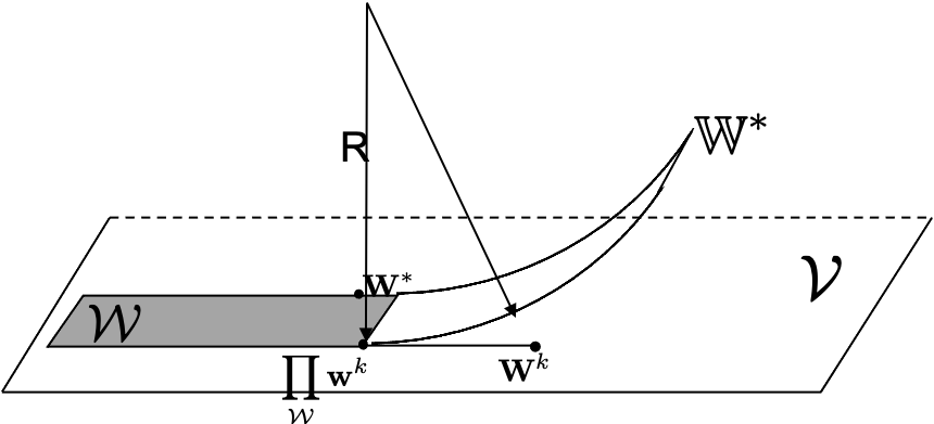
Refer to caption
Figure 3: If the support hyperplains intersect with angle 00 (exact cut), then the point 𝐖k\mathbf{W}^{k} can be arbitrarily close to the set 𝕎⋆\mathbb{W}^{\star} while remaining away from 𝒲\mathcal{W}.

In this section, we explain the high level intuition of why the intersection between the constrain set 𝕎⋆\mathbb{W}^{\star} and the feasible return vectors 𝒱\mathcal{V} needs to be nonsingular. The key problem arises from the fact that 𝕎⋆\mathbb{W}^{\star} is defined in space ℝd\mathbb{R}^{d} where the set of feasible return vectors 𝒱\mathcal{V} may not be of full dimension. In such cases, for the actual achievable constrain set of interest 𝒲=𝕎⋆∩𝒱\mathcal{W}=\mathbb{W}^{\star}\cap\mathcal{V}, there are too much freedom in selecting 𝕎\mathbb{W} as long as its elements on 𝒱\mathcal{V} remains fixed. In particular, an achievable return vector 𝐖K\mathbf{W}^{K} can be very far away from the constrained feasible set 𝒲\mathcal{W}, where as being arbitrarily close to the set 𝕎⋆\mathbb{W}^{\star}. The process is illustrated in Figure 3 by sending the radius RR to infinity. Note that 𝒲\mathcal{W} remains unchanged in this process. Since the cost is measured by the distance to 𝕎⋆\mathbb{W}^{\star} instead of to the actual set of interest 𝒲\mathcal{W}, the deviation from 𝐖\mathbf{W} to 𝒲\mathcal{W} cannot be reduced to 0 with any fixed algorithm given that point 𝐖\mathbf{W} is already very close to the target set 𝕎⋆\mathbb{W}^{\star}.

Quantifying the level of non-singularity is necessary, whereas lower bounding the angle at intersection is one natural way of many to do so.