Bayesian multiscale deep generative model for the solution of high-dimensional inverse problems

In this section, we introduce the inverse problems of interest and briefly discuss the limitations of standard Bayesian inference approaches to inverse problems. We consider a spatially-varying parameter $\bm{x}(\bm{s})$ usually represented as a random field $\bm{x}(\bm{s},\omega)$, where $\bm{s}$ is spatial location in the domain $\mathcal{S}$ and $\omega$ is a random event in the sample space $\bm{\Omega}$. This random field is discretized by a random vector $\bm{x}\in\mathbb{R}^{M}$ using standard finite element or finite difference discretization approaches. In our inverse problem setting, $\bm{x}(\bm{s})$, will be considered as our primary quantity of interest.

Let us consider a physical system governed by PDEs in a given spatial domain. We assume $\bm{x}(\bm{s},\omega)$ to be an input parameter (e.g. material property) of this model. Of interest to this work are distributed properties with multiscale features. The forward model concerning this physical system is usually considered as a function $\mathcal{F}:\mathbb{R}^{M}\rightarrow\mathbb{R}^{D}$, which maps the unknown parameters $\bm{x}$ to the observable output $\mathcal{D}_{obs}\in\mathbb{R}^{D}$ with a measurement noise $\bm{\xi}\in\mathbb{R}^{D}$:

The inverse problem is to infer the unknown parameters $\bm{x}$ based on these noisy data $\mathcal{D}_{obs}$. In the particular problem we will focus in Section 4, our goal is to estimate the permeability field in a porous media flow using pressure measurements.

Without prior information about the measurement system and/or model evaluation, we assume that $\bm{\xi}$ is a zero-mean Gaussian noise with covariance matrix $\bm{\Sigma}$, i.e., $\bm{\xi}\sim\mathcal{N}\left(\bm{0},\bm{\Sigma}\right)$. Since often $dim(\mathbb{R}^{D})\ll dim(\mathbb{R}^{M})$, the inverse problem is highly ill-posed and identification of the parameter $\bm{x}$ is highly-sensitive to this noise. The Bayesian paradigm [5] provides a general and natural way to treat the unknown parameter $\bm{x}$ as random variable to highlight the uncertainty in the inference process. Given the observation data $\mathcal{D}_{obs}$, one calculates the posterior probability $\pi(\bm{x}|\mathcal{D}_{obs})$ via Bayes’ formula as follows:

where $\pi(\bm{x})$ is the prior distribution, and $\mathcal{L}_{e}(\mathcal{D}_{obs}|\bm{x})$ is the likelihood function which evaluates the discrepancy between the forward predictions and observations. For the assumed case of Gaussian noise, we can define the likelihood function as

As the parameter $\bm{x}$ of interest is high-dimensional, the normalization constant in Eq. (2) involves computing a high-dimensional integral that is often an intractable process. Thus approximate inference for the posterior $\pi(\bm{x}|\mathcal{D}_{obs})$ is performed using the unnormalized density, i.e.,

Without a closed-form expression, the posterior distribution in Eq. (4) must be computed numerically. To this end, MCMC [10, 44] or other approximation methods like Ensemble Kalman filter (EnKF) [16, 30] are often employed. However, there are still two main difficulties for these methods. MCMC and EnKF implementations will often fail to directly approximate the posterior of the high-dimensional spatially-varying parameter $\bm{x}$. Moreover, for complex parameters (e.g. channelized permeability), the prior information cannot be easily cast as an explicit probability distribution. However, one often has access to a historical dataset $\bm{X}\equiv\{\bm{x}^{(i)}\}_{i=1}^{N}$ [16, 45, 46] where $\bm{x}^{(i)}$ can be seen as samples from the underlying prior distribution $\pi(\bm{x})$. One could use $\bm{X}$ to approximate $\pi(\bm{x})$ with its empirical measure. However, in this work, we will use this dataset to approximate the prior distribution with a generative model as follows:

where $p(\bm{z})$ is a simple distribution (e.g. Gaussian) for the latent variable $\bm{z}\in\mathbb{R}^{d}$, and $p_{\bm{\theta}}(\bm{x}|\bm{z})$ is a generative model parameterized by $\bm{\theta}$ (decoder). In a DGM like a VAE, one can choose a Gaussian distribution $\mathcal{N}(\bm{0},\bm{I})$ for $p(\bm{z})$, and $\mathcal{N}(\mu_{\bm{\theta}}(\bm{z}),\sigma^{2}\bm{I})$ for $p_{\bm{\theta}}(\bm{x}|\bm{z})$, where $\mu_{\bm{\theta}}(\bm{z})$ is the output of the decoder neural network, and $\sigma$ is a hyperparameter that does not depend on the latent variable $\bm{z}$. It is common practice in the literature [15, 16, 47, 48] to ignore the noise and approximate the density $p_{\bm{\theta}}(\bm{x}|\bm{z})$ with the point estimate $\mu_{\bm{\theta}}(\bm{z})$. Once the model is trained, we can thus define a mapping from the latent space to the original parameter space, i.e. $\bm{x}=\mu_{\bm{\theta}}(\bm{z})$.

The parameters $\bm{\theta}$ of the generative model $p_{\bm{\theta}}(\bm{x}|\bm{z})$ can be computed using the given training dataset $\bm{X}$ by minimizing the Kullback-–Leibler (KL) divergence $D_{KL}\left(\pi(\bm{x})||p(\bm{x}|\bm{\theta})\right)$ [49], where $\bm{x}^{(i)}\stackrel{{\scriptstyle i.i.d}}{{\sim}}\pi(\bm{x})$. This leads to the equivalent problem of maximizing the marginal log-likelihood:

The above marginalization is potentially very difficult to compute involving an intractable integration. Using Expectation-Maximization is also intractable as that will require the posterior $p_{\bm{\theta}}(\bm{z}|\bm{x})$ that is also computationally intractable. The marginal likelihood for the dataset $\{\bm{x}^{(i)}\}_{i=1}^{N}$ can be reformulated using a variational density $q_{\bm{\phi}}(\bm{z}^{(i)}|\bm{x}^{(i)})$ (encoder) parameterized by $\bm{\phi}$. The details of these calculations will be given in Section 3.3.

To approximate the posterior distribution in Eq. (4) using the MCMC method, we are interested to generate realizations sampled from the underlying prior distribution $\pi(\bm{x})$. To sample realizations from $\pi(\bm{x})$ using the generative model, one can sample $\bm{z}_{i}$ from the simple and low-dimensional distribution $p(\bm{z})$ and then obtain the realization $\bm{x}^{(i)}$ using the decoder model $\mu_{\bm{\theta}}(\bm{z})$. Alternatively, instead of approximating the posterior $\pi(\bm{x}|\mathcal{D}_{obs})$ in Eq. (4), one can instead evaluate the low-dimensional posterior $p(\bm{z}|\mathcal{D}_{obs})$ using the following unnormalized density:

where $p(\bm{z})$ is an explicit distribution, and the likelihood can be evaluated using the decoder model $\mu_{\bm{\theta}}(\bm{z})$ and the forward model $\mathcal{F}(\bm{x})$. The evaluation of the posterior of the low-dimensional latent variable $\bm{z}$ using MCMC or EnKF is computationally tractable [15, 16].

To further improve the efficiency of the inference process, we will introduce a multiscale version of the above highlighted generative model to perform inference in each scale $l=1,2,\ldots,L$ from the coarsest-scale ($l=1$) to the desired finest-scale ($l=L$). This multiscale scheme based on the MDGM contains a hierarchical simple distribution $p(\bm{z}_{l})$ at each scale $l$ and a conditional distribution $p_{\bm{\theta}_{l}}(\bm{x}_{l}|\bm{z}_{l})$ that can generate the spatially-varying parameter $\bm{x}$ in each scale. Correspondingly, one can assess the posterior $p(\bm{z}_{l}|\mathcal{D}_{obs})$ using MCMC with $p(\bm{z}_{l})$, $\mu_{\bm{\theta}_{l}}(\bm{z}_{l})$, and $\mathcal{F}_{l}(\bm{x_{l}})$. The details of this multiscale model are given next.

Our physical systems of interest are governed by a system of PDEs, and the spatially-varying property of interest is a material property appearing e.g. in the constitutive equations. The forward problem defines the well-posed solution of the PDEs (with some boundary conditions) given appropriate material properties. Such problems are often solved in a discretized fashion with finite element or finite difference or spectral approximations for different levels of discretization of the spatial domain $\mathcal{S}$. In this work, we are interested in a hierarchical parameterization of the spatially-varying parameters $\bm{x}_{l}$ with different spatial discretization or resolutions at each scale $l$. If the forward model is performed in the $2$-D space, the parameter random fields $\bm{x}_{l}$ at the $l$-th scale are treated as images, e.g. $\bm{x}_{l}\in\mathbb{R}^{H_{l}\times W_{l}}$ ($M_{l}=H_{l}\times W_{l}$), where $H_{l},W_{l}$ denote the number of the pixels in the horizontal and vertical directions, respectively.

For notational convenience, we assume that the finest scale parameters $\bm{x}_{L}$ represent our “true parameter model". The noisy observations $\mathcal{D}_{obs}$ in our numerical studies are taken from this discretization level. In the inverse problem of interest, our task is to compute $\bm{x}_{L}$ given a finite number of observations. For the solution of this inverse problem, prior knowledge can provide useful information for $\bm{x}_{L}$ before any observations. As prior information for our model, we assume that we are given a dataset $\bm{X}=\{\bm{x}^{(i)}_{L}\}_{i=1}^{N}$. To obtain images for training the generative model at different discretization levels, we will need to obtain a multiscale training dataset.

This can be accomplished by upscaling the fine-scale training dataset [50, 51, 52]. For example, with an upscaling (deterministic) operator $\mathcal{U}:\mathbb{R}^{M_{l}}\rightarrow\mathbb{R}^{M_{l-1}}~(M_{l-1}\ll M_{l})$, where $M_{l}$ and $M_{l-1}$ are the dimensions of $\bm{x}_{l}$ and $\bm{x}_{l-1}$, respectively. The dataset $\{\bm{x}^{(i)}_{l-1}\}_{i=1}^{N}$ in the coarse-scale $(l-1)$ is obtained by

The datasets $\{\bm{x}^{(i)}_{l}\}_{i=1}^{N},~l=1,2,\dots,L$ in different scales are obtained by adopting recursively $\mathcal{U}$ in Eq. (8) starting with the finest-scale $l=L$. we assume $\bm{x}^{(i)}_{l}$ is sampled from $l$-th scale underlying prior distribution $\pi_{l}(\bm{x}_{l})$. The operator $\mathcal{U}$ used in this paper is deterministic, which leads to a one-to-one correspondence between the elements in $\{\bm{x}^{(i)}_{1},\dots,\bm{x}^{(i)}_{L-1},\bm{x}^{(i)}_{L}\}_{i=1}^{N}$. One can choose different operators $\mathcal{U}$ depending on the particular parameter of interest. In this paper, we employ the arithmetic average¹¹ 1 http://www.epgeology.com/static-modeling-f39/how-upscale-permeability-t6045.html:

where $n_{e}$ denotes the number of elements in the fine-scale $l$ corresponding to one element in the coarse-scale $(l-1)$. The value at the coarse-grid element $e$ is the mean of the values in the spatially corresponding elements $e_{i}$ in the fine-scale. Spatial correspondence between two adjacent scales with $50\%$ coarsening in each direction is illustrated in Fig. 1.

An example illustrating this deterministic upscaling for channelized permeability using Eq. (9) is given in Fig. 2. The coarse-scale image provides a blurry representation of the fine-scale image but overall its features are consistent with those of the fine-scale image. It can be noticed that the coarse-scale image manifests itself with a checkerboard pattern that misses a lots of local information.

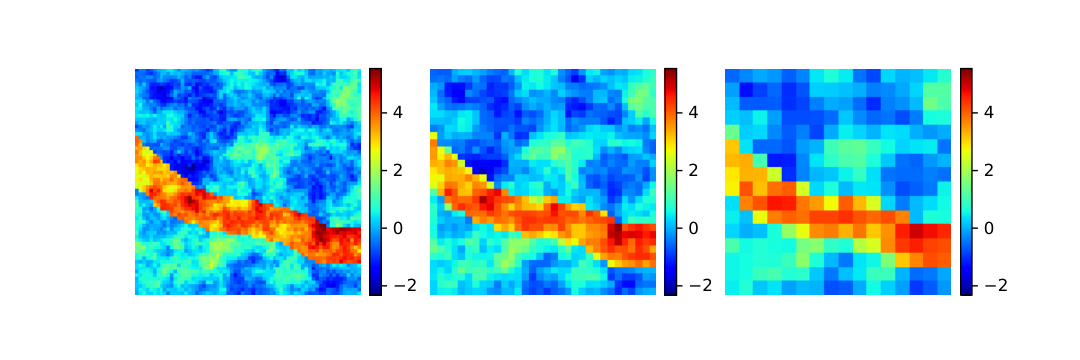
With the scales of interest pre-determined and the training dataset defined at each scale, we are ready to train the MDGM and perform inference on each scale using the proposed hierarchical multiscale framework.

Given the training dataset $\{\bm{x}^{(i)}\}_{i=1}^{N}$, we seek to learn a DGM that can approximate $\pi(\bm{x})$ with Eq. (5). The DGM involves the original parameter space and the latent space and the mappings between these spaces. For any $\bm{x}$ sampled from the underlying distribution $\pi(\bm{x})$, the corresponding $\bm{z}$ is sampled from the conditional distribution $q_{\bm{\phi}}(\bm{z}|\bm{x})$, where $q_{\bm{\phi}}(\bm{z}|\bm{x})$ is called the recognition model or probabilistic encoder model, and $\bm{\phi}$ are its model parameters. In the reverse direction, one can sample a $\bm{z}$ from a simple and low-dimensional distribution $p(\bm{z})$, and obtain the corresponding $\bm{x}$ from the generative model or probabilistic decoder model $p_{\bm{\theta}}(\bm{x}|\bm{z})$.

For high-dimensional inversion tasks, direct inference in the fine-scale is prohibited due to the computational cost of the forward model. In addition, inference of the latent parameters $\bm{z}$ that lead to good estimates of $\bm{x}$ through a generative model requires a high-dimensional $\bm{z}$. This will lead to long exploration costs for MCMC and requires a large number of forward model evaluations. To this end, given the multiscale dataset as discussed in Section 3.1, we propose a multiscale scheme for posterior estimation by introducing a hierarchy of generative models from coarse- to fine-scales. In this scheme, the coarse-scale generative models have low-dimensional latent spaces. This together with inexpensive forward model evaluations in the coarse-scales would allow MCMC to explore the posterior in coarse-scales with much reduced cost. The computational savings can be even higher if the latent representation on a given scale utilizes the latent information that was inferred in the immediately coarser-scale.

In our construct, the latent variables $\bm{z}_{l}$ at level $l$ of the hierarchy are given as $\bm{z}_{l}=(\bm{z}_{l-1},\bm{z}_{l}^{\star})$, where the latent variables $\bm{z}_{l-1}$ and $\bm{z}_{l}^{\star}$ are encoded from the coarse-scale parameter $\bm{x}_{l-1}$ and the fine-scale parameter $\bm{x}_{l}$, respectively. The latent variable $\bm{z}_{l-1}$ can generate $\bm{x}_{l-1}$ through the generative model at scale $(l-1)$. It also impacts the generation of $\bm{x}_{l}$ in the fine-scale $l$ by way of dominating its salient features since $\bm{z}_{l-1}$ captured the information from the immediately coarser-scale. In this setting with $\bm{z}_{l-1}$ encoded from $\bm{x}_{l-1}$, it is anticipated that $\bm{x}_{l}$ generated by $p_{\bm{\theta}_{l}}(\bm{x}_{l}|\bm{z}_{l-1},\bm{z}_{l}^{\star})$ would sustain most of the features of $\bm{x}_{l-1}$. We extend the Definition 3.1 to a multiscale scenario as follows.

Once the MDGM is established, the parameters $\bm{x}_{l}$ are encoded by the latent variable $\bm{z}_{l}$ so that one can perform inference of $\bm{z}_{l}$. Given the prior distribution $p(\bm{z}_{l})$, the decoder model $\mu_{\bm{\theta}}(\bm{z}_{l})$, the forward model $\mathcal{F}_{l}$, and observations $\mathcal{D}_{obs}$, inference of the posterior of $\bm{z}_{l}$ is performed as follows:

Note that MCMC converges and captures prominent and valuable features quickly in the coarse-scale $(l-1)$ since $\bm{z}_{l-1}$ is low-dimensional and the forward model $\mathcal{F}_{l-1}$ is less expensive in comparison to $\mathcal{F}_{l}$. For an efficient Bayesian inference at each scale $l$, we are interested in using the posterior distribution at coarse-scale $(l-1)$ to provide an informative prior information or improve sampling efficiency in the next finer-scale. This avoids relying completely on inference in a high-dimensional latent space where direct computation of fine-scale details would increase the model complexity. The purpose of inference on fine-scale is to correct the details rather than run long exploration for capturing all appropriate features. A related idea was implemented earlier using hierarchical structured sparse grids in [13]. In summary, the inverse problem is divided into a multiscale posterior estimation, with the inference of parameters proceeding from coarse- to fine-scale. The definition of the multiscale posterior estimation problem is given next.

The MDGM is used to generate parameters with different discretization/resolution. We construct such a model based on the variational autoenoder (VAE). The coarsest generative model that involves a single-scale ($l=1$) is vanilla VAE. It employs the dataset $\{\bm{x}_{1}^{(i)}\}_{i=1}^{N}$ (generated as discussed in Section 3.1) sampled from the underlying distribution $\pi(\bm{x}_{1})$, i.e. $\bm{x}_{1}^{(i)}\stackrel{{\scriptstyle i.i.d}}{{\sim}}\pi(\bm{x}_{1})$. We consider below the probabilistic generative model on a single-scale before deriving the multiscale formulation in Section 3.4. For simplicity of the notation, we drop the subscript $1$ in the equations below even though this model will be used in the scale $l=1$.

Given the training dataset $\{\bm{x}^{(i)}\}_{i=1}^{N}$, one can introduce a variational family $q_{\bm{\phi}}(\bm{z}|\bm{x})$ to convert the intractable computation of maximizing the marginal log-likelihood in Eq. (6) into an optimization problem, where $\bm{\phi}$ denotes the model parameters. It can be written as follows:

where the last step is the application of Jensen’s inequality. The above lower bound is called the variational lower bound. For a given training dataset, one can maximize the variational lower bound rather than the marginal log-likelihood. This is an optimization problem with respect to model parameter $\bm{\theta}$ and $\bm{\phi}$. The variational lower bound in Eq. (3.3) can be written as follows,

The minimization of the $-\mathcal{L}(\bm{\theta},\bm{\phi})$ balances the optimization of both the recognition and generative models. Thus the recognition model parameters $\bm{\phi}$ are learned jointly with the generative model parameters $\bm{\theta}$ [18]. The graphical model is shown in Fig. 3.

To evaluate $\mathcal{L}(\bm{\theta},\bm{\phi})$ in Eq. (12), there are three probability distributions to be identified. As mentioned in Definition 3.1, we shall select appropriate simple distributions for the latent variables $\bm{z}$. For example, in this paper, we let $p(\bm{z})\sim\mathcal{N}(\bm{0},\bm{I})$. The $\mathbb{E}_{\bm{z}^{(i)}\sim q_{\bm{\phi}}(\bm{z}^{(i)}|\bm{x}^{(i)})}[\log p_{\bm{\theta}}(\bm{x}^{(i)}|\bm{z}^{(i)})]$ in Eq. (12) is the expected log-likelihood. It encourages the reconstructed data $\hat{\bm{x}}$ by the decoder to approximate the original data $\bm{x}$. We assume $p_{\bm{\theta}}(\bm{x}|\bm{z})$ is modeled by a Gaussian distribution $\mathcal{N}(\mu(\bm{z}),\sigma^{2}\bm{I})$, where the mean $\mu(\bm{z})$ is the output of a decoder neural network and $\sigma$ is a constant hyperparameter that does not depend on the decoder so that it can be ignored during optimization. Let $\hat{\Sigma}=\sigma^{2}\bm{I}$, the first term in Eq. (12) then takes the form based on the minibatches:

where $n$ denotes the number of training samples of $\bm{x}$ (also referred to as the batch size in the training of deep neural networks). For each epoch, there are $\frac{N}{n}$ minibatches, each batch uniformly sampled from the dataset $\{\bm{x}^{(i)}\}_{i=1}^{N}$. $m$ is the number of $\bm{z}$ samples from $q_{\bm{\phi}}(\bm{z}|\bm{x})$ for an expectation approximation using the Monte Carlo method. One can also refer to Eq. (13) as the reconstruction error.

For the $D_{KL}(q_{\bm{\phi}}(\bm{z}^{(i)}|\bm{x}^{(i)})\|p(\bm{z}^{(i)}))$ in Eq. (12), $q_{\bm{\phi}}(\bm{z}^{(i)}|\bm{x}^{(i)})$ is taken as a Gaussian distribution, where the mean $\hat{\mu}(\bm{x})$ and the variance $\hat{\sigma}^{2}(\bm{x})$ are outputs of the encoder network. The KL-divergence can be analytically computed when both distributions are Gaussian [18]. The KL-divergence works as an objective function for the optimization problem with respect to the encoder parameters $\bm{\phi}$. Based on the minibatches, it can be written as:

where $\hat{\mu}_{k}(\bm{x})$ and $\hat{\sigma}_{k}(\bm{x})$ denote the $k$-th element of the mean and standard deviation, respectively, which are outputs of the encoder network. The results of Eqs. (13) and (14) summarize the objective function for optimization of the encoder and decoder neural networks.

Inspired from $\beta$-VAE [53], we slightly modify the underlying loss function. This modification of the VAE results by adding an extra hyperparameter $\beta$ to the KL divergence. This hyperparamter can constrict the capacity of the latent bottleneck and encourage a disentangled representation. We would like the individual dimensions of the latent variable $\bm{z}$ to be interpretable or to correspond to some features of parameters thus disentangling the true variation of data [53, 54]. A good interpretability and factorized representation for the latent variable will facilitate the feature exploration in MCMC. Note that [55] has shown that $\beta$-VAE is an important method in disentangled representation for learning the compositional and hierarchical visual concept. Choosing an appropriate hyperparameter $\tilde{\beta}$ for loss function is important in MDGM. We can define the loss function $\tilde{\mathcal{L}}\equiv-\frac{n}{N}\mathcal{L}(\bm{\theta},\bm{\phi})$ in each training iteration, the loss function for the single-scale probabilistic generative model as follows:

To optimize the parameters $\bm{\theta}$ and $\bm{\phi}$ in neural networks, one could employ stochastic gradient descent (SGD) or other gradient-based optimization algorithms related to back propagation. Note that the second term in Eq. (15) is an expectation approximation using the Monte Carlo method that samples $\bm{z}^{(i,j)}$ from $q_{\bm{\phi}}(\bm{z}^{(i,j)}|\bm{x}^{(i)})$. But the expectation computation involving sampling with a high variance will reflect on the gradient estimation, which leads to an unfavorable influence on optimization. To make it trainable and back propagate the gradient correctly, the reparameterization trick is introduced. The latent variables $\bm{z}$ are expressed by a differentiable transformation $g_{\bm{\phi}}(\epsilon,\bm{x})$ with respect to an auxiliary independent random variable $\epsilon$. In the Gaussian distribution case, we let $\epsilon\sim\mathcal{N}(0,I)$, sampling $\bm{z}$ via such a $g_{\bm{\phi}}(\epsilon,\bm{x})$:

where $\odot$ refers to an element-wise product. The illustration of forward and back propagation computation with the reparameterization trick is shown in Fig. 4.

As discussed in Definition 3.1, we constructed the probabilistic models $p_{\bm{\theta}}(\bm{x}|\bm{z})$ and $q_{\bm{\phi}}(\bm{z}|\bm{x})$ to sample $\bm{x}$ given its corresponding latent variable $\bm{z}$ and to map the parameters $\bm{x}$ to the latent space, respectively. Based on the objective function in Eq. (15) and neural network in Fig. 4 (detailed architecture see A), one can optimize the network parameters $\bm{\phi}$ and $\bm{\theta}$. The implementation procedure is summarized in Algorithm 1.

This model only involves a single-scale parameter representation learning, while MDGM is a multi-stage and recursive training procedure from coarse to fine, i.e. the training output in the coarse-scale model is the input to the next finer-scale model. The coarsest-scale probabilistic models $p_{\bm{\theta}_{1}}(\bm{x}_{1}|\bm{z}_{1})$ and $q_{\bm{\phi}_{1}}(\bm{z}_{1}|\bm{x}_{1})$ are outputs of Algorithm 1. The generative model $p_{\bm{\theta}_{1}}(\bm{x}_{1}|\bm{z}_{1})$ is used for the estimation of the posterior $\pi(\bm{x}_{1}|\mathcal{D}_{obs})$ in the coarsest-scale by standard MCMC (see Section 3.5). The recognition model $q_{\bm{\phi}_{1}}(\bm{z}_{1}|\bm{x}_{1})$ is the input (as a pre-trained model) to the second-scale ($l=2$) generative model training (see Section 3.4).

In Section 3.3, we presented the single-scale parameter generative model in a probabilistic perspective and discussed how to use deep neural networks for its implementation. In this section, we enhance this model to a multiscale framework. Based on the parameter data generation procedure in Section 3.1, we start from the training data in the finest-scale and coarse grain them recursively to represent the training data in the coarsest-scale. We demonstrate the MDGM by explaining how to train it in the $l$-th scale as an example based on the assumption that we obtained the pre-trained encoder and decoder networks in the $(l-1)$-th scale.

To construct the connection among various scales, we design a special latent space for the finer-scale. In particular, its latent variable $\bm{z}_{l}$ inherits the latent variable $\bm{z}_{l-1}$ of the previous scale and augments it with an additional latent variable $\bm{z}_{l}^{\star}$. These two variables are independent. This is in principle similar to the Bayesian approach followed in [13] where a hierarchical sparse grid approximation was used to represent an unknown parameter field at different scales.

As we discussed in Definition 3.2, we also need to train the recognition model $q_{\bm{\phi}}(\bm{z}_{l}|\bm{x}_{l})$ and generative model $p_{\bm{\theta}}(\bm{x}_{l}|\bm{z}_{l})$ in scale $l$ with the same objective function as in Eq. (6). The difference with standard generative models is that the recognition model is divided into two parts in order to encode the parameter $\bm{x}$ with the independent latent variables $\bm{z}_{l-1}$ and $\bm{z}_{l}^{\star}$. As shown in Fig. 5, the encoder network includes a pre-trained encoder network and an augmented encoder network. $q_{\bm{\phi}}(\bm{z}_{l-1}|\bm{x}_{l})$ is computed by adopting the upscaling operator over $\bm{x}_{l}$ firstly and then using the previous scale encoder network. It can be modeled by

Since the upscaling operator $\mathcal{U}$ is deterministic, we can write the following:

As in the single-scale probabilistic generative model in the last section, the variational lower bound $\mathcal{L}(\bm{\theta},\bm{\phi};\bm{x})$ consists of two parts as described in Eq. (12), i.e. $\mathbb{E}_{q_{\bm{\phi}}(\bm{z}^{(i)}|\bm{x}^{(i)})}[\log p_{\bm{\theta}}(\bm{x}^{(i)}|\bm{z}^{(i)})]$ and $D_{KL}\left(q_{\bm{\phi}}(\bm{z}^{(i)}|\bm{x}^{(i)})||p_{\bm{\theta}}(\bm{z}^{(i)})\right)$. The first part in the $l$-th scale is formulated as the reconstruction error introduced in Eq. (13), which involves the decoder model $p_{\bm{\theta}_{l}}(\bm{x}_{l}|\bm{z}_{l})$ and its model parameter $\bm{\theta}_{l}$. The second part is much distinct with $p(\bm{z}_{l})$ being the target distribution in the KL-divergence. It is an isotropic multivariate Gaussian distribution as well, but it can be viewed as the joint distribution of $(\bm{z}_{l-1},\bm{z}_{l}^{\star})$, where $\bm{z}_{l-1}$, $\bm{z}_{l}^{\star}$ are independent. Thus $p(\bm{z}_{l-1})$ and $p(\bm{z}_{l}^{\star})$ are also isotropic multivariate Gaussian distributions. Combining with Eq. (18), we rewrite the KL-divergence as follows:

where $\bm{\phi}$ in the $l$-th scale is $\bm{\phi}_{l}$ containing $\bm{\phi}_{l-1}$ and $\bm{\phi}_{l}^{\star}$, where $\bm{\phi}_{l-1}$ denotes the parameters of the encoder network $q(\bm{z}_{l-1}|\bm{x}_{l-1})$ in the $(l-1)$-th scale and $\bm{\phi}_{l}^{\star}$ denotes the parameters of the augmented encoder network $q(\bm{z}_{l}^{\star}|\bm{x}_{l})$ in the $l$-th scale. Recall that we need to employ the pre-trained encoder network $q_{\bm{\phi}_{l-1}}(\bm{z}_{l-1}|\bm{x}_{l-1})$ directly in the $l$-th scale training because it should ensure that the finer-scale generative model shares common latent variables $\bm{z}_{l-1}$ with the coarser-scale, so

We also use gradient-based optimization algorithm to train the MDGM where the back propagation is only applied in the decoder network and augmented encoder network as blue arrows illustrated in Fig. 5. We can formulate the loss function for each training iteration like Eq. (15) as follows:

where $\hat{\mu}_{lk}(\cdot)$ and $\hat{\sigma}_{lk}(\cdot)$ denote the $k$-th element in the mean and standard deviation, respectively, which are outputs of the $l$-th scale augmented encoder network, and $\mu_{l}(\cdot)$ is the output of the $l$-th scale decoder network. Here, $m$ is still set to be $1$ when the batch size $n$ is large enough. $d_{l}^{\star}$ is the dimension of the latent variable $\bm{z}_{l}^{\star}$. The hyperparameter $\tilde{\beta}$ is determined by balancing the disentanglement of the parameter features and reconstruction.

In summary, assume that we obtained the probabilistic encoder and decoder models in the previous $(l-1)$ level. We can then train the augmented encoder network and decoder networks using the objective function in Eq. (21) so that the probabilistic encoder $q_{\bm{\phi_{l}}}(\bm{z}_{l}|\bm{x}_{l})$ and the probabilistic decoder $p_{\bm{\theta}_{l}}(\bm{x}_{l}|\bm{z}_{l})$ in the $l$-th scale are acquired. For details see Algorithm 2. The architectures of the augmented encoder and decoder networks are the same as those in the encoder and decoder networks for the single-scale model (refer to A).

We have introduced so far the probabilistic generative model in a single-scale in the last section and the concept of generative modeling across two scales in this section. Since these unsupervised learning models only need the unlabeled data, we only provide the finest-scale dataset $\{\bm{x}^{(i)}_{L}\}_{i=1}^{N}$ sampled from the underlying prior distribution $\pi(\bm{x}_{L})$ and adopt the deterministic upscaling operator $\mathcal{U}$ to generate the dataset in the scale of interest. The training of the generative models proceeds from the coarsest- to the finest-scale. The coarsest-scale generative model is trained by Algorithm 1. From the second- to the finest-scale, the generative model is trained recursively by Algorithm 2. Once the generative models are trained in the scales of interest, they can be integrated with MCMC to estimate the posterior of the parameters in each scale.