When to Quit Gambling, if You Must! Thanks: We thank Nick Barberis for a long list of constructive comments on a previous version of the paper that have led to a much improved version.
Abstract
We develop an approach to solve Barberis 2012’s casino gambling model in which a gambler whose preferences are specified by the cumulative prospect theory (CPT) must decide when to stop gambling by a prescribed deadline. We assume that the gambler can assist their decision using an independent randomization, and explain why it is a reasonable assumption. The problem is inherently time-inconsistent due to the probability weighting in CPT, and we study both precommitted and naïve stopping strategies. We turn the original problem into a computationally tractable mathematical program, based on which we derive an optimal precommitted rule which is randomized and Markovian. The analytical treatment enables us to make several predictions regarding a gambler’s behavior, including that with randomization they may enter the casino even when allowed to play only once, that whether they will play longer once they are granted more bets depends on whether they are in a gain or at a loss, and that it is prevalent that a naivité never stops loss.
Key words: casino gambling; cumulative prospect theory; optimal stopping; probability weighting; time inconsistency; randomization; finite time horizon; Skorokhod embedding; potential function.
1 Introduction
Barberis 2012 proposes a casino gambling model in the framework of Tversky and Kahneman 1992’s cumulative prospect theory (CPT) to study the optimal timing to quit gambling and leave the casino. The author has derived two key economic insights: (1) a CPT gambler may be willing to enter the casino even though its bets offer neither positive expected values nor skewness because, by implementing an appropriate stopping strategy, he would be able to build a positively skewed final winning amount that would be favored by the underlying probability weighting in CPT; (2) there is an inherent time-inconsistency due to the dynamically changing strength of probability weighting on a same event: the gambler may deviate completely from his initial stopping strategy as he gambles along, and his eventual stopping behavior depends on whether he is aware of this time-inconsistency and whether he is able to commit his original plan.11 1 Barberis 2012 discusses three types of gamblers, following the original classification of Strotz 1955: a naïve gambler who is unaware of the time-inconsistency and changes his strategy all the time; a precommitted gambler who is aware of time-inconsistency and can commit to his initial plan; and a sophisticated gambler who is aware of time-inconsistency yet unable to commit, and at each time takes the future selves’ disobedience into account when devising an optimal strategy.
It is, however, not an objective of Barberis 2012 to develop a general approach to solve the casino model he puts forward. Barberis 2012 acknowledges that the nonlinear probability weighting involved in CPT makes it “very difficult” to solve the problem analytically, and “the problem has no known analytical solution for general ” (p. 42), where is an exogenously given number of bets the gambler can maximally have. Instead, Barberis 2012 uses an exhaustive search to find a solution; namely, he enumerates all the possible Markovian stopping strategies, calculates the CPT value of each of them and finds the one that achieves the highest CPT value as the optimal strategy. As one would expect, this approach works only for smaller , as the number of admissible Markovian strategies is exponential in .22 2 The number of nodes is in a binomial tree of horizon , and at each node there is a binary choice of {stop, continue}. Hence the total number of strategies is . Barberis 2012 solves the problem with .33 3 We ran exhaustive search on a desktop with Intel Core i5-4590/CPU 3.30GHz/RAM 8.00GB for different ’s while keeping the other parameters same as Barberis 2012’s. The running times for were 39 seconds, 771 seconds and 27 hours, respectively. We were unable to obtain the solution for due to out of storage, with the running time estimated to be 300 days.
Naturally, to better understand the implications of a model it is important to have a systematic approach to solve it, not necessarily in an analytically closed form, but in a computationally efficient way.44 4 Consider, e.g., the simplex method for linear programs or the dynamic programming formulation for optimal control problems. Not only can we then obtain optimal solutions for arbitrary values of parameters, but we may gain (likely more profound) economic insights from the model by post-optimality analyses such as comparative statics. The main technical hurdle to solve the casino model is probability weighting, as pointed out by Barberis 2012. The two main approaches in the classical optimal stopping theory – dynamic programming (variational inequalities) and martingale method – both fail under probability weighting: the former does because of the time-inconsistency, and the latter does because of the absence of a “tower property” with respect to the weighted probability.
He et al. 2017, He et al. 2019b, He et al. 2019a are probably the first series of papers that aim at an analytical treatment of the casino model, albeit in the infinite time horizon.55 5 Here by “analytical treatment” we mean an optimization analysis not based on heuristics or on brute force such as an exhaustive search. The main idea of these papers consists of two deeply intertwined steps: (1) search the optimal probability distribution of the final winning/losing amount upon leaving the casino instead of the optimal time to leave; (2) once the optimal distribution is found, recover the optimal time that generates it.66 6 This idea was first put forth by Xu and Zhou 2012 for a continuous-time optimal stopping model featuring probability weighting. There is considerable difficulty to adapt this idea to the discrete-time setting. Both steps call for a complete characterization of the set of all the admissible distributions, and the second step is the discrete-time version of the eminent Skorokhod embedding theorem which in the casino setting is solved in He et al. 2019b. The main thrust to make this idea work is to permit randomization, namely the gambler can flip an independent, possibly biased, coin to assist his decision each step of the way. The probabilities of the head of the coin are endogenous and dynamically changing; thus they are part of the final solution.77 7 Mathematically, randomization convexifies the aforementioned set of admissible distributions. Hence, He et al. 2017, He et al. 2019a use randomization as a technical tool to make the Skorokhod embedding work, but fall short of explaining, economically, why people would randomize and how exactly they do it. The present paper offers discussions on these issues; see Subsection 2.3. The randomization of decisions is a key feature when studying agents with CPT preferences, as discussed independently by Henderson et al. 2017. He et al. 2017, He et al. 2019a also allow path-dependent strategies, that is, the stopping decision is made based on the whole betting history instead of just the current winning/losing amount. They further show that allowing path-dependent strategies or randomized ones strictly improve the optimal CPT values. Based on these analyses, He et al. 2019a turn the casino model into an infinite dimensional mathematical program that can be solved fairly efficiently. Most of the gambler’s behaviors – those of a precommitter and of a naiveté – implied from the solutions reconcile qualitatively with Barberis 2012’s results; but there are also new findings. For example, it is revealed that, for most empirically relevant CPT parameter estimates, a precommitted gambler lets gain run while stops loss, but a naïve one almost surely does not stop at any loss level.
As noted, He et al. 2017, He et al. 2019a deal with the infinite horizon gambling model. There are important reasons to study the finite horizon model under CPT preferences, despite the existing results for the infinite horizon counterpart. Conceptually, the finite horizon problem approximates the reality much better, as a gambler clearly will not be able to play arbitrarily and indefinitely long. Also, the original work of Barberis 2012 considers and hence we need to solve the finite horizon model in order to be able to make a direct comparison. It is worth noting that solutions to the finite horizon case can not be recovered from those of the infinite horizon case by a simple truncation: if is optimal for the latter, then, typically, will not be optimal for the former.
Methodologically, the finite horizon case is significantly more complex. It is well acknowledged that optimal stopping in a finite horizon is fundamentally more difficult than its infinite horizon counterpart, mainly because value function of the former has both time and spatial variables while the latter has only spatial variables. In the infinite time horizon setting in which the accumulated winning/losing amount is modelled by a symmetric random walk , He et al. 2019b show that for any centered probability measure on the set of integers , there exists a randomized stopping time such that ’s distribution is .88 8 In the terminology of Skorokhod embedding theorem, we say embeds in . As discussed previously, this is the key theoretical underpinning for the new approach. Unfortunately, this result is no longer true if the stopping time is constrained by a pre-specified deadline. Indeed, additional conditions are required for measures that can be embedded by uniformly bounded stopping times. One of the contributions of this paper is to identify explicitly these conditions, which in turn enables us to reformulate the original casino model into a mathematical program whose number of constraints is of the order of and, hence, can be efficiently solved.
Once we have an algorithm to solve the gambling model for any parameter values, we will then be able to first compare our results with those of Barberis 2012’s. In particular, we compute for exactly the same case that is solved and discussed in Barberis 2012 with . The respective stopping strategies for a precommitter are identical except in two time–state instances in which our decisions are to stop with very small probabilities (0.00864 and 0.0368 respectively) whereas Barberis’ are just to continue. Qualitatively, both strategies are of the so-called loss-exit type, namely, they continue in gains but stop after having accumulated sufficient amounts of losses. With randomization, our optimal CPT value improves, if slightly, over Barberis’. Likewise, the respective naïve strategies are the same save for one time–state instance in which ours is to stop with a probability of 0.179 while Barberis’ is to continue. Our solution, however, enables us to look beyond the relatively short horizon of . Indeed, we carry out numerical experiments for different values of up to , and discover that the interplay between the utility function, probability weighting and loss aversion dictates various gambling behaviors.
Note that our analytical treatment relies on the introduction of randomization in our model, as randomization convexifies the optimization problem. Barberis 2012 does not allow randomization, for which our approach would fail. However, our solution would provide a well-founded relaxation heuristic for solving a casino model without randomization: we first relax the problem by introducing randomization, and then, for each time-state pair, round up or round down the probability of stopping to 1 (which means stop) or to 0 (which means continue).
Our approach makes it possible to analyze and understand the impacts of some key attributes of the model, which we believe is the most important contribution of this paper. For example, Barberis 2012 argues that a gambler may be willing to enter a casino because, by implementing a loss-exit strategy, he may be able to generate a positively skewed probability distribution of the final accumulated gain/loss which has a positive CPT preference value. However, he will need to spend time building such a skewed distribution, which requires a sufficiently large . We show, however, that for the same gambler who would have demanded a long horizon for agreeing to enter the casino, will enter even if he is allowed to play only once (i.e., ), provided that he can flip a coin. The reason for this is that, with randomization, the gambler can design a coin right away with the desired skewed distribution, saving all the time otherwise needed to reach that distribution. Another insight is about the value of time: how much is time on your hands worth? Specifically, we examine the question of what a gambler would do should he be allowed to stay one more period than previously agreed. Would he always take advantage of this extended time horizon and actually play the additional round? It turns out that there is no uniform answer to the question – it depends crucially on whether the gambler is currently in a gain or at a loss.
We also study the behaviors of a naïve gambler with various parameter specifications and a longer time horizon (). We find that, unless he does not enter the casino, his behavior is consistently of gain-exit type, i.e., he stops gain but lets loss run, reminiscent of the disposition effect in security trading (Odean 1998). In particular, he never stops loss and gambles “until the bitter end”. This gamble-until-the-bitter-end behavior is derived by Ebert and Strack 2015 in a model in which a naïve gambler can construct arbitrarily small random payoffs. Because he prefers “skewness in the small”, he never stops gambling. Henderson et al. 2017, employing the approach developed in Xu and Zhou 2012, investigate a stylized continuous-time model and show that a naïve gambler may stop with a positive probability if she is allowed to randomize, which complements and counters the findings in Ebert and Strack 2015. Both Ebert and Strack 2015 and Henderson et al. 2017 rely on the crucial feature of their models that allows the gambler to construct arbitrarily small random payoffs. This feature is absent in our discrete-time model, in which the gambler cannot construct strategies with arbitrarily small random payoffs due to the minimal stake size fixed to be $1. Hence, their results are not applicable to our setting. Our finding therefore suggests that the gamble-until-the-bitter-end phenomenon is probably more prevalent of a naivité’s behavior.
The paper proceeds as follows. In Section 2, we formulate a casino gambling model under CPT as an optimal stopping problem and discuss why we allow randomization in our model. In Section 3, we develop the key step in our approach to solve the gambling model: characterizing the set of probability distributions of all possible accumulated winning/losing amounts upon leaving the casino. In Section 4, we present a mathematical program that is equivalent to the casino model, and then report the results of a numerical example which is studied in Barberis 2012. We discuss about various implications and predictions of our model in Section 5. Finally, we conclude the paper by Section 6. Proofs are placed in Appendices.
2 The Model
In this section we first highlight the key ingredients of Tversky and Kahneman 1992’s CPT, then formulate the casino gambling model in a finite time horizon as an optimal stopping problem, and finally discuss about the reasons why we make randomization available in our model.
2.1 Cumulative prospect theory
In CPT, a utility (or value) function depends on a reference point in wealth that divides gains and losses. An agent derives the utility from gains and losses, rather than from the absolute amount of wealth itself. The utility function is
where and are both concave functions and . This renders an overall S-shaped utility function that is concave (risk-averse) in the gain region and convex (risk-loving) in the loss region . Moreover, yields that, for the same magnitude of a gain and a loss, the agent is more sensitive to the latter, a notion termed loss aversion. Tversky and Kahneman 1992 propose the following parametric form of :
| (1) |
where and ; see the left panel of Figure 1 for an illustration of this type of functions.
In CPT there are also probability weighting (or distortion) functions and applied to gains and losses respectively. An inverse S-shaped weighting function is first concave and then convex in the domain of probabilities. Such a weighting function overweights both tails of a probability distribution, reflecting the exaggeration of extremely small probabilities of extremely large gains and losses. Tversky and Kahneman 1992 suggest a parametric form of a weighting function :
| (2) |
where ; see the right panel of Figure 1 for an illustration. Note that means that no weighting is applied.
2.2 Formulation of a casino gambling model
We now reformulate Barberis 2012’s model of casino gambling in a finite time horizon , where is given. The gambling process proceeds as follows. At time 0, the gambler is offered a fair bet, e.g., one with a roulette wheel: win or lose $1 with equal probability.99 9 As in Barberis 2012, we assume in this paper that the gamble is fair. It will not affect the main economic findings and implications of our results. A model of unfair games is more technical, and is left for a future study. If the gambler decides not to play the bet, then he will not even enter the casino. If the gambler enters and takes the bet, then the bet outcome is played out at time 1, leading to either a win or a loss of $1 at time 1. At that time the gambler is offered the same bet again and he decides whether to play. If he declines the bet, then the game is over and the gambler leaves the casino with $1 gain or loss. This process continues in the same fashion until time : the bet is offered and played out repeatedly until either the first time the gambler declines the bet, or at time when the gambler must quit gambling and leave. The accumulated gain/loss process can be represented as a binomial tree; see Figure 2. Therein, each node is marked by a pair , where stands for the time and the amount of cumulative gains or losses. For example, the node signifies a cumulative loss of $2 at time 2. The process has a terminal time but the gambler may quit at some earlier time .

The gain/loss binomial tree is a standard symmetric random walk (SSRW) defined on a filtered probability space . We assume the probability space is rich enough to support an -measurable random variable that is uniformly distributed on and independent of .
Suppose the gambler quits gambling at a random time . Then, with the reference point being his initial wealth before he enters the casino, the CPT value of his wealth upon leaving is
| (3) | ||||
Throughout this paper we assume that both and are concave and both and are inverse S-shaped. The gambler needs to determine the optimal time to quit and leave the casino: such a stopping (exit) strategy is made at to maximize among all admissible strategies. Note that, due to probability weighting, the problem is inherently time-inconsistent; so is optimal only at in the sense of a precommitted strategy; it may no longer be optimal from the vantage point of any later time .
We now define precisely the set of admissible stopping strategies
So a decision whether or not to quit at time depends on all the information up to . In particular, path-dependent strategies are admissible. Moreover, – and hence all – contains the information about , a uniform random variable independent of . Using , we can define countably many binary random variables which are mutually independent and also independent of . In consequence, an admissible strategy may involve randomization by tossing a (generally biased) coin. In the next subsection we will outline the rationale behind allowing randomized strategies.
The gambler’s problem is
| (4) |
2.3 Randomization
In our model (4), the filtration includes the information based on a uniform random variable that is independent of the underlying random walk. This means that we allow the gambler to assist his decision by flipping an independent, most likely biased, coin at each node.1010 10 Note any random variable taking a continuum of values, including the Bernoulli random variable, can be generated from a uniform random variable. We now discuss the rationale behind making this randomization available in our model.
First of all, randomization is related to the accommodation of path-dependence. It is practically more reasonable, and indeed necessary, to consider path-dependent strategies than mere Markovian ones. How has the gambler arrived at a current amount (say $500) – whether he has won big first and then lost most of them, or he has gradually accumulated this amount by many small wins – clearly might affect his decision. As a matter of fact, almost all our decisions in life are made based on all the information, past and present, rather than just on the current state of affair. After all, being Markovian is just a mathematical assumption and convenience that aims to dramatically reduce the dimension of the underlying problem or, in a continuous-time setting, turns an infinite dimensional problem into a finite dimensional one. Path-dependence is also a standard formulation in optimal stopping theory (see, e.g., Shiryaev 1978) and indeed in general stochastic control theory (see, e.g., Yong and Zhou 1999). Now, He et al. 2017 shows that any non-randomized, path-dependent stopping time is equivalent to a randomized, Markovian stopping time in the sense that both attain the same CPT value.1111 11 While this result has been obtained for the infinite horizon model, the underlying argument is exactly the same for the finite horizon case. The intuition is that, due to the independent increments of a random walk, considering all the past information can be achieved by randomizing at the current state. As a result, we can consider randomization in lieu of considering the past information.
However, He et al. 2017 also show the converse is not true, namely, a randomized Markovian strategy may not be replicated by a non-randomized, path-dependent strategy, and the optimal CPT value among the former type may be strictly greater than that among the latter type. The authors attribute this to the lack of quasi-convexity of CPT preference (in contrast to the classical expected utility theory preference). This property was also exploited by Henderson et al. 2017 to complement and counter the findings in Ebert and Strack 2015.
So, what are the other reasons why a gambler may want to randomize, beyond and independent of replacing path-dependence and maximizing CPT preference? Indeed, preference for randomization is observed in daily life and in different cultures, such as last-minute deals by flight booking apps, “sushi omakase” (you entrust yourself to a sushi chef to choose the ingredients and presentations of your sushi plate), and “fukubukuro” (grab bags filled with unknown and random contents). The practice of “drawing divination sticks”, popular in Chinese culture even today, is a vivid example of seeking randomization in addition to religious reasons. When people are reluctant or unable to make their own decisions on important matters (usually marriage, school, or even home move), they go to a temple, pray and draw divination sticks, and follow whatever words on the sticks tell them to do.
There are also rich literatures in experimental psychology and economics that document extensive experiments about individuals deliberately randomizing when making decisions. Agranov and Ortoleva 2017 report on experiments in which subjects who face identical questions repeated three times in a row often switch between their answers, and a significant portion of them are even willing to pay for a coin flip to choose answers for them. Dwenger et al. 2013 study a clearing house data for university admissions in Germany, where applicants submit multiple rankings of the universities they wish to attend. The authors find that a significant fraction of students report contradictory rankings without any rational reasons.
The psychological literature has put forward various theories to explain the preference for randomization, such as responsibility aversion (Leonhardt et al. 2011), decision avoidance (Anderson 2003), and regret theory (Zeelenberg and Pieters 2007). In the aforementioned example of divination sticks, prayers delegate their decisions to a god, a benefit of which is to release themselves from making the decisions on their own and hence relieve themselves from regret should the choice turn out to be bad. In the economics literature, Diecidue et al. 2004 use the general ‘‘utility of gambling” to explain randomization.1212 12 The theory of utility of gambling can also be used to explain why a gambler is willing to play a bet that has unfavorable average return; see Barberis 2012. Here, the utility of gambling is applied to a different phenomenon, namely, the desire to randomize. This type of utilities either violate some basic axioms underlining classical utility theory such as second-order stochastic dominance and betweenness (Camerer and Ho 1994, Blavatskyy 2006) (precisely the same reason why randomization strictly improves CPT value), or prefer irrational diversification or hedging (Rubinstein 2002), or weight more on fairness than on outcomes (Kahneman et al. 1986, Bolton et al. 2005).
In summary, a gambler may have various independent reasons to perform randomization while gambling, which may be only partly relevant, or completely irrelevant, to his CPT preference. That is why we introduce an independent binary random variable to capture such a desire for randomization. Finally, the easy availability for flipping a biased coin nowadays also makes the inclusion of randomization more plausible. For complex gambles such as stock trading, one can easily simulate the outcomes of any randomization in a computer. For literal casino gamble, the gambler can bring in a smartphone where apps are available to simulate coin flips with any user-defined probabilities.
3 Characterization of Stopped State Distributions
As explained earlier, the main thrust of our approach to solving Problem (4) is to change its decision variable from the stopping time to the distribution of the stopped state . A key step is therefore to characterize the admissible set of these distributions. Moreover, once an optimal distribution is obtained there needs to be a way to recover the stopping time that generates this distribution. These two questions are intertwined and will actually be solved together. This section addresses them.
Denote by the set of probability measures on and by the subset of whose elements have finite first moments and are centered: and . Denote by the subset of supported on integers.
For , define a function
which is called the potential of .1313 13 Note that our definition here is the negative of the usual definition of potential. For , is a linear interpolation of the points . The following are evident:
| (5) |
Potential function uniquely determine probability measure, namely, two measures are identical if and only if their potential functions are identical; see Obłój 2004. Finally, for any stopping time , with a slight abuse of notation we simply write for the potential of the distribution of , when well defined.
We can use a sequence of piecewise linear functions, called evolutional functions, to approach a potential function. Indeed, given , we define recursively the following sequence of functions:
| (6) |
We then extend each to non-integers by linear interpolation. When is fixed, we may drop the superscript and just write for simplicity. Figure 3 illustrates how evolves to for an example of .
The optimal stopping time we will derive belongs to a special class of randomized, Markovian stopping times called the Root stopping times. The original version of the Root stopping times was developed in Root 1969 to solve the classical Skorokhod embedding problem for a Brownian motion on an infinite time horizon.1414 14 Precisely, an (original) Root stopping time is the first hitting time of on an explicitly constructed region with a barrier in the time-space . For any centred on with a finite second moment , such a time exists which embeds in , i.e., and ; see Root 1969, Rost 1976 and Obłój 2004. We now develop the analogous ideas in discrete time for the SSRW.
Consider an integer-valued vector where, for any , with some , and another vector , where . Given and , define the probability distributions of a family of Bernoulli random variables as follows:
Graphically, is a barrier that defines a time-space stopping region
and the components of are the probabilities to stop exactly on the boundary of this stopping region. The randomized Root stopping time is defined as
| (7) |
This stopping time is Markovian, because it depends only on the current state of the random walk . It is randomized because it depends on the outcome of the Bernoulli random variables ’s.
Figure 4 illustrates such a stopping time. The grey boundary divides the area into two subareas: the one on the left hand side has white nodes representing “continue”, and that on the right hand side consists of black nodes indicating “stop”. Stopping at a grey node is randomized with being the probability of stopping.

The following theorem is one of the main results of the paper that provides a theoretical foundation for the numerical algorithm we are going to present to solve our casino gambling model. It characterizes the admissible set of stopped distributions under stopping times in , and reveals that the set is the same as that of stopped distributions using only randomized Root stopping times. As a consequence, any admissible stopping strategy is always dominated by a randomized Root stopping time.
Theorem 3.1
Let , such that . Then there exists a stopping time such that if and only if
| (8) |
Moreover, in this case there exists a randomized Root stopping time such that .
4 A Mathematical Program
Theorem 3.1 hints that we can, instead of endeavoring to find the stopping time in Problem (4), try to find the probability distribution of the stopped state . Namely we change decision variable from to for Problem (4). The resulting problem is a (nonlinear) mathematical program (i.e., a constrained optimization problem) with the condition (8) translating into certain constraints.
Moreover, once we solve this problem and find the optimal distribution , then it follows from Theorem 3.1 that there exists a randomized Root stopping time that achieves the same stopped distribution and, hence, solves (4). Furthermore, based on the proof of Theorem 3.1 (see Appendix A), we can devise an algorithm to find and, consequently, . We now formulate the mathematical program and provide its solution algorithm.
4.1 The mathematical program formulation and solution
Given , let . Define two -dimensional vector variables, and , where , , . Clearly, and are gambler’s decumulative gain distribution and cumulative loss distribution, respectively. Then the original objective function (3) is equivalent to, as a function of ,
| (9) |
Naturally, we must have , , . On the other hand, has zero expectation due to optional sampling theorem; so
In summary, the following constraints are required for the probability distribution of where :
| (10) |
Moreover, Theorem 3.1 necessitates condition (8), which constitutes a family of inequalities on ’s potential function and the corresponding evolutional functions, which will later be translated into constraints on ’s distribution functions. Here, let us illustrate (8) for each of . To ease notation, we will suppress the superscript on the evolutional functions. For , the condition is satisfied automatically for any with . For , (8) amounts to . For , (8) reduces to
For , (8) is equivalent to
For , (8) specializes to
The following lemma, which follows a direct, if somewhat lengthy, computation, expresses and, consequently, the constraints (8), in terms of and .
Lemma 4.1
For ,
To illustrate, take . Then
We are now ready to formulate the mathematical program that is equivalent to the original stopping problem (4). Define
along with a set of functions , , , in the following way. For , let
and for :
Then, the mathematical program is
| (11) |
The number of decision variables ( and ) and the number of constraints in (11) are both linear in ; hence the complexity of the problem is manageable. Moreover, there are standard solvers to solve this type of mathematical program.1515 15 In the following numerical experiments, we employ nonlinear optimization solver ‘fmincon’ from MATLAB Optimization Toolbox, on a desktop with Intel Core i5-4590/CPU 3.30GHz/RAM 8.00GB. For the Barberis 2012’s parameters , , with , MATLAB uses 205 seconds, 220 seconds, 280 seconds, 350 seconds respectively. (Compare with those of the brute force reported in Footnote 3.) The running times for are 9.35 minutes, 29 minutes, 89 minutes, 3.5 hours, 7.17 hours, respectively.
The running times for were 39 seconds, 771 seconds and 27 hours, respectively. We were unable to obtain the solution for due to out of storage, with the running time estimated to be 300 days.
Once we solve this problem to get optimal , we then run the following algorithm to find the optimal randomized Root stopping time:
Step 1 Given , compute the corresponding potential function: for , and for . Then, compute its evolutional functions by (6), .
Step 2 Compute the boundary that separates the “continue” region from the “stop” region: , . (The constraints in (11) guarantees that the set involved is non-empty and .)
Step 3 Compute the probability to stop at the boundary:
Step 4 Construct according to (7).
4.2 A numerical example
We present an example to illustrate the solution procedure, using the same parameters as in Barberis 2012 with , , , .1616 16 More examples with much longer time horizons will be presented in the next section. Solving the corresponding mathematical program for the optimal distribution yields
The corresponding potential function is
Figure 5 illustrates how is achieved by the evolutional functions within five steps.
We then apply the algorithm previously presented to recover the optimal randomized Root stopping time from the optimal distribution , with . The strategy, which is optimal at (only) and implemented by the precommitted gambler, is drawn in the left panel of Figure 6. Note that black nodes mean “stop”, white ones mean “continue”, and grey ones mean “randomization”. The number above a grey node is the probability to stop.
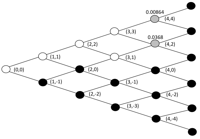

The main feature of this precommitted optimal strategy is to continue in the gain domain and to stop in the loss domain until , except at time 4 where there are positive probabilities to stop in gains. In particular, randomization takes place at nodes and , with the (very small) probabilities to stop equal to 0.00864 and 0.0368, respectively. The CPT value of this randomized strategy is 0.3369592. Compared with Barberis 2012 where the CPT value is 0.3369398, the optimal non-randomized, Markovian strategy has white nodes at and , instead of grey nodes that involve randomization.1717 17 These are the only two nodes that are different between Barberis 2012 and the present paper. Note they occur at and when there are sufficient gains. The intuition why the gambler randomizes at these two nodes will be explained in Subsection 5.3 when we investigation the situation when the horizon is extended from to . In summary, allowing path-dependent and randomized strategies does indeed improve optimal CPT values (albeit only slightly in this particular instance) over non-randomized, Markovian ones.1818 18 This improvement can be significant with other parameter specifications. For example, with and , the optimal CPT value among non-randomized, path-independent strategies is 0.058069135, and that among randomized ones is 0.065696808, representing a 13% increase. When and , the corresponding figures are 0.0253839 and 0.0492624, representing a 94% increase.
Moreover, one can achieve this improved optimal value by implementing a Markovian randomization, with the overall strategy very similar qualitatively to Barberis 2012’s -- both are of the loss-exit type.1919 19 We have also revisited the example considered also in He et al. 2017. In that paper, a randomized strategy, found by trial and error, leads to the value function compared with for the best non-randomized strategy. Using our algorithm, we see that the best randomized strategy actually gives . It is still a loss-exit type and it stops at node with probability , node with , node with and node with .
While the precommitted gambler follows through the optimal strategy originally determined at time 0, a naïve gambler thought he would do the same but in actuality constantly deviates from previously planned strategies. More precisely, at any time , a naiveté re-considers the optimal stopping problem starting from , devises a precommitted strategy but carries it out for only one period (because he will re-optimize again at the next time instant). Here, we assume this gambler keeps his initial wealth at time 0 as the reference point.2020 20 This is also the assumption made in Barberis 2012 when analyzing a naïve gambler’s behavior. It is both natural and plausible that a gambler remembers the initial amount of cash he brought into the casino and always compares wins and losses against that amount. The naïve gambler’s strategy can be computed by deriving all the time- precommitted strategies, , implementing each of them for just one period, and then “pasting” them together. As a result, his actual quitting strategy could be drastically different from the precommitted one, the one he originally planned before he enters the casino; see the right panel of Figure 6. There, the only node calling for randomization is now (2,0), with a probability of 0.179 to quit.2121 21 This is also the only node that makes our naïve strategy different from Barberis 2012’s in which the node (2,0) is white meaning “continue”; see the right panel of Figure 4 therein. Comparing the two strategies depicted in Figure 6, we find that the naïve strategy is not only significantly different from the precommitted one, but indeed almost completely opposite in character: the latter is mainly to continue in the gain domain and to stop in the loss domain, while the former is reversed. For a discussion on experimental evidence on the dramatic departure of the actual gambling behaviors from the planned ones, see Barberis 2012. Heimer et al. 2020 presents strong evidence from lab and field that supports the inconsistent dynamic framework of Barberis 2012. In the context of stock trading, such a naïve behavior – the tendency of selling winners too soon and keeping losers too long – is widely observed especially for retail investors, and is termed the disposition effect by Odean 1998.
5 Discussions
5.1 To enter or not to enter: the power of randomization
One of the main takeaways of Barberis 2012 is that CPT offers an explanation why a gambler would be willing to enter a casino even if the bets there have neither skewness nor positive expected values. By implementing a loss-exit strategy, namely keep gambling when winning but stop gambling when accumulating a sufficient loss, he envisions a positively skewed probability distribution of the accumulated gain/loss at the exit time which is favored by the CPT preference. However, he would need a sufficiently long time period to build such a skewed distribution in order to have a positive CPT value to justify the entry (recall that the CPT value of not playing at all is zero). For the case of a piece-wise power utility function (1) and an inverse S-shaped weighting function (2), Barberis 2012 provides a sufficient condition for this to happen.2222 22 Barberis 2012 is stated for a naïve gambler. However, the result holds for a precommitter as well because both gamblers face the same problem at . Moreover, for the parameter values , , , this sufficient condition translates into ; see Barberis 2012.2323 23 These parameter values are close to those given by Tversky and Kahneman 1992, i.e., , , , . If we apply the exact Tversky and Kahneman 1992 parameter values to Barberis 2012, then the corresponding . Such a shorter period is expected because the probability weighting in gains is stronger than that in losses with Tversky and Kahneman 1992’s parameters; thus it takes less time to build the desired positively skewed distribution with a positive CPT value.
However, with randomization allowed, the gambler may be willing to enter the casino even if he is allowed to play only once (i.e., ).
Proposition 5.1
Suppose . If , then the optimal CPT value is strictly positive.
Recall that in our model, randomization is available; so the optimal CPT value being strictly positive means that the gambler will enter the casino, possibly tossing a coin to decide whether to actually play (the only) one round of bet.
What if ? Naturally, as increases, the optimal CPT values increase. Figure 7 graphs the optimal CPT values for with the Tversky and Kahneman 1992 estimates. Therefore, if the gambler will enter the casino for with a given set of parameters, so will he for with the same parameters. As a consequence, Proposition 5.1 holds for as well.
It is straightforward to show that for the weighting function (2), when (which is the case with Tversky and Kahneman 1992’s estimates), we have . Hence, Proposition 5.1 yields that, as long as the loss-aversion degree is finite, a randomized gambling strategy is always preferred to non-gamble, even when .
The intuition of Proposition 5.1 is as follows. The condition means that exaggeration of big gains outweighs exaggeration of big losses and loss aversion combined; so the gambler assigns a positive CPT value to a sufficiently positively skewed distribution. Without randomization, it would take time to build such a distribution. With randomization, however, the gambler can design a coin right away with such a distribution, saving him all the time otherwise needed. In other words, a coin toss can be used to supersede all the time-consuming (and perhaps clever) maneuvers to reach the desired distribution. Note that even though randomization still gives rise to a symmetric distribution of gains and losses and hence the loss aversion seemingly would prevent the gambler from entering, the sufficiently unequal levels of probability weighting on gains and losses, as stipulated by the condition , yields the contrary.
On the other hand, the effectiveness of randomization crucially depends on the chosen parameters. If the degree of probability weighting in gains is equal to or less than that in losses, and the level of loss-aversion is sufficiently large so that , then the above proposition does not apply because . For example, for utility function (1) and probability weighting function (2), let , , , the values used in Barberis 2012. In this case, we find a positive CPT value of randomized strategies only when the time horizon is at least , slightly shorter than that () presented in Barberis 2012 using a special non-randomized loss-exit strategy. The corresponding optimal precommitted strategy is also of a loss-exit type: stop once losing $1, and continue with possible randomization when wining. If we further let the probability weighting in gains be weaker than that in losses, e.g., and , then a positive preference value is found only at .
5.2 Alpha, delta, and lambda
There are three components in the risk/loss preferences under CPT: the utility function, the probability weighting and the loss aversion. They are intertwined and compete with each other in determining the overall preference and dictating the final behavior. In this subsection, we study the roles they play in the case when the utility function is (1) and the weighting function is (2), with parameters , and .
Others being kept unchanged, the effect of each of these parameters is as follows: a smaller implies a higher degree of risk-aversion in gains and a smaller implies a higher degree of risk-seeking in losses, a smaller yields a higher level of probability weighting in gains/losses, and a smaller indicates a smaller extent of loss aversion. To understand the overall impact of these parameters on exit decisions, we first fix and consider four sets of scenarios: large and small ; small and large ; small and small ; and large and large . Then we examine the effect of . In the following discussions we fix .
The left panel of Figure 8 draws the optimal precommitted strategy when , and . These are the same parameters as in the numerical example presented in Subsection 4.2, except now we have a much longer horizon. Again, black nodes mean “stop”, white nodes “continue”, grey nodes “randomize”, and the number above the grey node is the probability to stop. This strategy is mainly to continue or toss a coin in gains until the final time and to stop in losses, which is thus a loss-exit one. The intuition is as follows. This is the case where are relatively large (lower risk-aversion/-seeking) and relatively small (heavier probability weighting). In the gain region, the stronger exaggeration of the small probability of winning a large amount outweighs the weaker risk aversion; hence the gambler is willing to take more risk and stay longer. In the loss region, the stronger exaggeration of the small probability of losing a large amount, together with the loss aversion, outweighs the weaker risk-seeking appetite and prompts the gambler to play safe and quit earlier.


The above argument is reversed, leading to a gain-exit type of strategy, when are relatively small and relatively large, such as the one depicted in the left panel of Figure 9 where , , . An interesting small variation of this case is when probability weighting is absent, i.e., , , , in which the optimal CPT value is positive and the precommitted strategy is still a gain-exit one. Indeed, a positive preference value is found at a much shorter horizon under this group of parameters, and the optimal distribution of is left-skewed (which is favored by a strong risk-seeking preference in losses represented by ).


The left panel of Figure 10 shows the precommitted strategy for the parameter values and , which is the case of small and small . This is still a loss-exit strategy, but the main differences from that visualized by the left panel of Figure 8 are that, in the gain region, there are now more black nodes and the numbers above the grey nodes are larger, implying a higher likelihood of stop even when the gambler has accumulated a gain. The reason is that with a smaller , the exaggeration of the small probability of winning a large amount still outweighs the risk aversion in gains, but with a lesser degree than the previous case.


The last set of parameters are , , with which the optimal CPT value is zero and the gambler will simply not enter the casino. This is because these parameter values render a risk preference close to both risk-neutral and probability–weighting–free, while a zero-mean bet and a loss-aversion degree prevent the gambler from playing the game at all.
The impact of is more straightforward, which we now examine. For each group of and considered above, we obtain the optimal CPT value by varying from 1 to 3; see Figure 11, the left panel. Quite naturally, each of the optimal CPT values decreases as increases, and three of them hit zero before reaches 3. As a result, the gambler will be increasingly reluctant to stay in or even enter the casino as his level of loss aversion increases.
The analysis in this subsection shows that the CPT casino modeling with various constellations of parameter specifications can predict and explain a rich array of gambler behaviors. In particular, whether the strategy is loss-exit or otherwise depends on the interplay between the three intertwining and competing forces represented by , , and .
5.3 One more round?
With a longer time horizon a precommitter is more likely to obtain a positive CPT preference value and hence more likely to enter the casino because, trivially, the optimal CPT value for is no less than that for . On the other hand, with a longer time horizon and a loss-exit strategy one can possibly construct a more positively skewed probability distribution of the accumulated gain/loss at the exit time which, under CPT preference, is preferred by the precommitter. Hence, the optimal preference value may strictly increase as increases, which is demonstrated in the right panel of Figure 11 where the optimal CPT values for under different groups of parameters are plotted.
So, the overall CPT value will be heightened if the gambler is told to be granted an additional round of bet than previously agreed. But would he always take advantage of this extended time horizon and actually play the additional round? It turns out that the answer can be totally different depending on whether the gambler is in the gain region or in the loss region.
Let the original problem have a horizon and be a given exiting strategy. Assume and consider the scenario in which the gambler has reached the upper most node under , namely and . Now suppose the time horizon is expanded to so the gambler is allowed to play one more round. Firstly, we are interested in knowing, given and , namely the gambler has already played the originally final bet with the maximal possible accumulated win of , whether the gambler would actually take this opportunity and play one more time to possibly achieve a final accumulated gain of or .2424 24 Bear in mind all the decisions are made at as we are considering precommitted strategies. So we are studying this problem from the vantage point of . The situation is illustrated in the left panel of Figure 12. Recall that randomization is allowed at any time; so let us denote by the probability to stop at , and by the strategy appending the original by, given and , playing one more round with probability at time and finally stopping at time . Let . The decumulative distribution of differs from that of only at and . The problem now is to choose to maximize or, equivalently, to maximize
For large enough, both and are small enough to fall into the concave region of the probability weighting function . Hence the above is a concave maximization and the following first-order condition is necessary and sufficient for a maximum :
or equivalently,
| (12) |
Assuming is strictly concave (e.g. that given by (1)), the right hand side of (12) is strictly greater than one. Hence, the equation is satisfied by some , but not (noting ) or . Recall that and correspond to and respectively. So, given the gambler has already played until the end with a sufficiently accumulated gain (so that is sufficiently small), once he is allowed to play (only) one more time he will not have a black-and-white decision of either “continue” or “stop”; rather he will always engage in randomization to make his decision.2525 25 This also explains why randomization happens at in the gain region when he has one final bet to play, as the left panels of Figures 6, 8, 10 indicate. Moreover, as increases the right hand side of (12) decreases; hence increases or decreases. In other words, the more gains accumulated, the more likely the gambler will continue.


What is the intuition behind these results? Standing at , the probability of reaching the top most node and winning sufficiently large is very small; hence the effect of exaggeration of this small probability kicks in. Then, given the opportunity of an extra play, tossing a coin to decide is better than not playing at all, for the same reason as entering the casino even if one is allowed to play only once (see Subsection 5.1). Moreover, the more gains the stronger probability weighting, and hence more likely to play. On the other hand, playing this additional bet without tossing a coin (i.e., definitely continuing) is not optimal either because of the strict risk aversion – randomization helps trigger probability weighting in large gains which in turn offsets the risk aversion level.
Next, let us examine whether the gambler would like to take one more step in the loss region if the horizon is expanded. Again, suppose is a given exit strategy for the horizon , and denote . Let , where is the probability to stop at , and by the strategy extending the original by, given and (see the right panel of Figure 12 for an illustration), playing one more round with probability at time and stopping at time , assuming the horizon is now . Then a similar analysis to the gain case shows that the optimal minimizes
| (13) |
Different from the gain region, in the loss region the optimality is achieved by minimizing a concave function when is sufficiently small. Hence, the optimal is either or , corresponding to “stop” or “continue” respectively. This means that the gambler will not flip a coin this time. To investigate which is better between “stop” and “continue”, we calculate the difference between the objective values (13) at and at :
As , we have and, hence,
assuming is given by (2) with and has diminishing marginal (dis)utility, namely, as (which holds for (1)). This implies that the value (13) at is smaller than that at , when is sufficiently large. Consequently, the gambler will choose to stop even if he is offered to play one more round. The intuition is clear: from the perspective at , the probability of losing sufficiently big is very small, which is inflated by probability weighting. This inflation outweighs the risk-seeking in losses because of the diminishing marginal disutility. As a result, the action of stop, which generates zero additional CPT value, is the best because any other action will only add negative CPT values.
We have proved the following result.2626 26 We have put the proof of this result here instead of in the appendix, not only because it is relatively elementary, but also because the proof discloses why there are essential differences between the gain and loss regions.
Theorem 5.1
Let be a given strategy.
- (a)
Assume that is strictly concave and . Construct a new strategy , where , is a Bernoulli random variable that is independent of and , and . Then and, for sufficiently large , there exists such that .
- (b)
Assume that is given by (2) with , as , and . Construct a new strategy , where , is a Bernoulli random variable that is independent of and , and . Then and, for sufficiently large , for all .
For general utility and weighting functions, the above results are valid for sufficiently large ; but for the utility function (1) and probability weighting function (2) with Tversky and Kahneman 1992’s estimates, does not need to be excessively large. For example, it follows from the proof of (a) that all we need is to ensure falls into the concave domain of . For , this requires (refer to the right panel of Figure 1) which is satisfied when . Similarly, by the proof of (b), for and , a straightforward calculation yields that when , falls into the concave domain of and dominates the other choices.
In the preceding discussions we assume that an original (i.e., before the horizon is extended) strategy has resulted in the maximum possible gain or loss. We now investigate the situations when the strategy ends up with an intermediate state with a mild accumulated gain or loss. Specifically, let be a given exiting strategy and be a gain state. Assume and and consider the scenario in which the gambler has reached the node under , namely and . Now, with an additional round of play granted, we denote by the strategy modifying the original by, given and , playing one more round with probability at time , where . Let . An argument similar to the case of yields that the extra CPT value due to the possible additional round of play, as a function of , is
| (14) |
whose first-order derivative is
| (15) |
The necessary condition for a maximum is thus
| (16) |
Assume is sufficiently large so that falls into the concave region of . Because due to the strict concavity of , will never satisfy (16); hence or the gambler will not continue decisively. Moreover, if , then there is such that holds, in which case indicating that the gambler will randomize. On the other hand, if then it follows from (15) that (14) is a non-increasing function of ; so its maximal value achieves at (and hence ). This is in stark contrast to the case when : at some intermediate gain state , the gambler may indeed choose to stop even if the time horizon is extended.2727 27 This is examplified by the black node (9,1) in the left panel of Figure 10.
Finally, at an intermediate loss state , a similar analysis yields that randomization with is again being dominated. It is possible that (resp, ), in which case the gambler will continue for sure if the time horizon is extended. This is different from the case of maximal loss state .
5.4 Naïve gamblers
While a precommitted gambler follows the optimal strategy determined at time 0, a naïve gambler constantly deviates from it. We have shown in Subsection 4.2 that, under the parameter specification therein, the naiveté’s actual behavior changes from the originally planned loss-exit strategy to an eventual gain-exit one.
Numerically, the naivité’s strategy can be obtained by computing each time- precommitted strategy, carrying it out for just one period, and then pasting them together; see Subsection 4.2 for details. We apply this scheme to the first three groups of parameters studied in Subsection 5.2, and draw the naïve strategies in the right panels of Figure 8 – 10.
The problem in Figure 8 has the same parameter values as that in Figure 6 but a longer horizon. The changes from the left panels to the right ones in the two figures are qualitatively the same, namely the naivité turns a loss-exit strategy to a gain-exit one eventually. The same happens to Figure 10.2828 28 In the right panel of Figure 10, all the nodes with state are black, which “block” the gambler from accessing the nodes beyond state 1. This is why the nodes above state 1 are also all black. In Figure 9, the two panels are almost identical – both are gain-exit – except the two lowest nodes at . This is because the difference in behaviors of the precommitter and the naivité emanates from time-inconsistency, which in turn stems from probability weighting. In this case, the strength of probability weighting is very low with , leading to a low level of time-inconsistency than the other two cases and hence the high similarity between the precommitted and naïve strategies.
It is very interesting to note that, in all the cases, the naïve gambler’s behavior is consistent, irrespective of the underlying parameter specifications: once he enters the casino he always takes gain-exit strategies, reminiscent of the disposition effect in security trading. In particular, he never stops loss and gambles “until the bitter end” (Ebert and Strack 2015).2929 29 We reiterate that the result of Ebert and Strack 2015 depends critically on the assumption that the gambler can construct arbitrarily small random payoffs, which is possibly valid only in a continuous-time model. The finding that “gamble-until-bitter-end” is also present in the discrete-time casino model suggests that the behavior is probably more prevalent characterizing broadly a naivité (be it a gambler or an investor).
We now provide a theory that explains such a phenomenon. Suppose a naïve gambler has accumulated a gain equal to at time , the date just before the terminal one. Then his decision problem regarding whether he should quit at can be formulated as
where, as before, and is the probability to stop. Suppose satisfies the so-called subcertainty, i.e., for , a property that is proposed by Kahneman and Tversky 1979 and shared by many probability weighting functions including (2). Then
where the second inequality follows from the concavity of , while the equality is achieved when , corresponding to the decision of “stop”. We have established the following result.
Proposition 5.2
Assume that satisfies subcertainty. Then it is optimal for a naïve gambler to stop in gain at .
Next, suppose the naivité’ has accumulated a loss at . His decision problem to continue or stop at is
Suppose probability weighting function is differentiable and for , with the left hand side in the sense of limit for . A straightforward calculation verifies that this condition is satisfied by the Tversky–Kahneman weighting function (2). Then
where the last inequality comes from the concavity of . As a result, is non-increasing in and the minimum is achieved when , corresponding to the “continue” decision.
Proposition 5.3
Assume that is differentiable and for . Then it is optimal for a naïve gambler to continue in loss at .
A corollary of Proposition 5.3 is that the naivité will definitely continue even if there is only one round of play left as long as he is in loss, let alone when a longer horizon is allowed. As a consequence, he will not stop loss in any case, until the bitter end.
5.5 Sophisticated gamblers
A sophisticated gambler is unable to precommit and realizes that her future selves will deviate from whatever plans she makes now. Her resolution is to compromise and choose consistent planning in the sense that she optimizes taking the future disobedience as a constraint. Consequently, strategies of sophisticated gamblers can be obtained using backward deduction as in dynamic programming.
To start, we note that at , a sophisticated gambler and a naïve one face the same problem; hence we have the following immediate result.
Next, we derive a sophisticated gambler’s stopping strategies for the four cases studied in Subsection 5.2, where . It turns out that, of the four cases, she will enter the casino only in the case when , corresponding to Figure 9. Moreover, her strategy is identical to the one depicted in the right panel of Figure 9, which is the actual strategy of the naïve gambler and close to the precommitted strategy. This is because when is close to 1, the level of probability weighting is low, hence so is that of time-inconsistency, leading to similar strategies of all the three types of gamblers.
Note that in the case above, the sophisticated gambler takes the gain-exit type of strategy. Indeed, so long as she enters the casino, she essentially stops in gain under some mild conditions. This follows from the following argument: by Proposition 5.4, the sophisticated gambler will stop in gain at . Knowing this, she will also stop in gain at by virtue of exactly the same reason. Inductively, this leads to an overall gain-exit type of strategy.
On the other hand, the sophisticated gambler always stops no later than her naïve counterpart does. This is because while the latter solves an optimal stopping problem at every node, the former solves the same problem but with constraints from her future selves’ decisions. Hence, if the latter finds that stopping immediately is optimal at a current node, so will the former because the strategy of an immediate stop automatically satisfies the aforementioned constraints.
Proposition 5.5
Under any specification of parameters, a sophisticated gambler stops no later than a naïve gambler does.
An implication of this result is that the naivité is at least as risk-taking as the sophisticated, if not more.
5.6 Finite horizon versus infinite horizon
This section explores connection between the finite horizon and infinite horizon casino models.
Define
which is the set of admissible stopping strategies (allowing randomization) in the infinite time horizon. Suppose is optimal for the infinite horizon model and achieves a finite CPT value. Then we have
We see immediately that the value of the finite horizon model converges to that of the infinite horizon one as the horizon approaches infinity. The following makes this formal.
Theorem 5.2
Assume achieves the optimal value of the gambling model in the infinite time horizon with a.s., , and is lower-bounded a.s. Then
We stress that this result only reveals the relationship between the two models in terms of the optimal values. It does not offer a solution to the finite horizon problem (which is harder) from a solution to the infinite one (which is comparatively easier), nor does it tell the error in the optimal values when is given and fixed. That said, the result suggests that the optimal value of the infinite horizon model is an upper bound of that of the finite horizon one, and it is a tight upper bound if is sufficiently large. Moreover, while the truncation method mentioned earlier does not provide an exact optimal solution to the finite horizon model, it does nevertheless offer a good solution when is large enough.
6 Conclusion
In this paper we develop a systematic approach to studying the stopping behaviors of CPT gamblers in a finite time horizon. We hope that this work opens an avenue of thoroughly understanding Barberis 2012’s model and beyond. Indeed, as Barberis 2012 points out, casino gambling is not an isolated model requiring a unique treatment; rather it is just one of the many examples, including ones in financial markets, that share a common feature of the probability weighting.
References
- (1)
- Agranov and Ortoleva (2017) Agranov, M. and Ortoleva, P. (2017). Stochastic choice and preferences for randomization, Journal of Political Economy 125(1): 40–68.
- Anderson (2003) Anderson, C. J. (2003). The psychology of doing nothing: Forms of decision avoidance result from reason and emotion, Psychological Bulletin 129: 139–167.
- Barberis (2012) Barberis, N. (2012). A model of casino gambling, Management Science 58(1): 35–51.
- Blavatskyy (2006) Blavatskyy, P. R. (2006). Violations of betweenness or random errors?, Economics Letters 91(1): 34–38.
- Bolton et al. (2005) Bolton, G. E., Brandts, J. and Ockenfels, A. (2005). Fair procedures: Evidence from games involving lotteries, Economic Journal 115: 1054–1076.
- Camerer and Ho (1994) Camerer, C. F. and Ho, T.-H. (1994). Violations of the betweenness axiom and nonlinearity in probability, Journal of Risk and Uncertainty 8: 167–196.
- Diecidue et al. (2004) Diecidue, E., Schmidt, U. and Wakker, P. P. (2004). The utility of gambling reconsidered, Journal of Risk and Uncertainty 29: 241–259.
- Dwenger et al. (2013)
Dwenger, N., Kübler, D. and Weizsacker, G. (2013).
Flipping a coin: Theory and evidence.
Working Paper.
http://ssrn.com/abstract=2353282. - Ebert and Strack (2015) Ebert, S. and Strack, P. (2015). Until the bitter end: on prospect theory in a dynamic context, American Economic Review 105(4): 1618 – 1633.
- He et al. (2017) He, X. D., Hu, S., Obłój, J. and Zhou, X. Y. (2017). Path-dependent and randomized strategies in barberis’ casino gambling model, Operations Research 65(1): 97–103.
- He et al. (2019a) He, X. D., Hu, S., Obłój, J. and Zhou, X. Y. (2019a). Optimal exit time from casino gambling: Strategies of pre-committed and naive gamblers, SIAM Journal on Control and Optimization 57(3): 1845–1868.
- He et al. (2019b) He, X. D., Hu, S., Obłój, J. and Zhou, X. Y. (2019b). Two explicit skorokhod embeddings for simple symmetric random walk, Stochastic Processes and their Applications 129(9): 3431–3435.
- Heimer et al. (2020)
Heimer, R., Iliewa, Z., Imas, A. and Weber, M. (2020).
Dynamic inconsistency in risky choice: Evidence from the lab and
field.
Working Paper.
https://ssrn.com/abstract=3600583. - Henderson et al. (2017) Henderson, V., Hobson, D. and Tse, A. (2017). Randomized strategies and prospect theory in a dynamic context, Journal of Economic Theory 168(3): 287–300.
- Kahneman et al. (1986) Kahneman, D., Knetsch, J. L. and Thaler, R. (1986). Fairness as a constraint on profit seeking: Entitlements in the market, American Economic Review 76: 728–741.
- Kahneman and Tversky (1979) Kahneman, D. and Tversky, A. (1979). Prospect theory: An analysis of decision under risk, Econometrica 47(2): 263–291.
- Leonhardt et al. (2011) Leonhardt, J. M., Keller, R. L. and Pechmann, C. (2011). Avoiding the risk of responsibility by seeking uncertainty: Responsibility aversion and preference for indirect agency when choosing for others, Journal of Consumer Psychology 21: 405–413.
- Obłój (2004) Obłój, J. (2004). The skorokhod embedding problem and its offspring, Probability Surveys 1: 321–392.
- Odean (1998) Odean, T. (1998). Are investors reluctant to realize their losses, Journal of Finance 53(5): 1775–1798.
- Root (1969) Root, D. H. (1969). The exitstence of certain stopping times on brownian motion, The Annuals of Mathematical Statistics 40(2): 715–718.
- Rost (1976) Rost, H. (1976). Skorokhod stopping times of minimal variance, Sḿinaire de Probabilitś X, Vol. 511 of Lecture Notes in Mathematics, Springer, pp. 194–208.
- Rubinstein (2002) Rubinstein, A. (2002). Irrational diversification in multiple decision problems, European Economic Review 46: 1369–1378.
- Shiryaev (1978) Shiryaev, A. (1978). Optimal Stopping Rules, Springer–Verlag, New York.
- Strotz (1955) Strotz, R. (1955). Myopia and inconsistency in dynamic utility maximization, The Review of Economic Studies 23: 165–180.
- Tversky and Kahneman (1992) Tversky, A. and Kahneman, D. (1992). Advances in prospect theory: Cumulative representation of uncertainty, Journal of Risk and Uncertainty 5(4): 297–323.
- Xu and Zhou (2012) Xu, Z. Q. and Zhou, X. Y. (2012). Optimal stopping under probability distortion, Annals of Applied Probability 23(1): 251–282.
- Yong and Zhou (1999) Yong, J. and Zhou, X. Y. (1999). Stochastic Controls: Hamiltonian Systems and HJB Equations, Springer, New York.
- Zeelenberg and Pieters (2007) Zeelenberg, M. and Pieters, R. (2007). A theory of regret regulation 1.0, Journal of Consumer Psychology 17(1): 3–18.
Appendix
Appendix A Proof of Theorem 3.1
We prove this theorem through a series of results. We start by recalling some properties of the potential and its link to the first exit times.
Proposition A.1
Let be an -stopping time such that is uniformly integrable. Then
- (i)
For any , is a convex function, , with .
- (ii)
For any two integers and , , and is linear on .
- (iii)
Fix and let . Then
(17) In particular, if is odd, then for any odd ; and if is even, then for any even .
Proof.
The first two properties are standard; see Obłój 2004. So we only establish (iii). Note that is supported on . We have so that . In particular, since is a martingale, we have . Now take . Since , using (5), we have
| (18) |
Rearranging and observing that the thesis follows. ∎
The following proposition provides some useful properties of .
Proposition A.2
Let and . Then
- (i)
, .
- (ii)
when is odd and is even, or when is even and is odd.
- (iii)
is convex in and non-decreasing in .
Proof.
(i) By the construction of we have . On other hand, by (5) and the structure of SSRW that , one can show easily that , . Then by induction, we have .
(ii) Again, by construction we have for all odd and for all even . The conclusions follow immediately from induction.
(iii) Clearly is convex. Suppose is convex and fix . If we put for , pick any
and finally define by a linear interpolation for , then is convex. Observe that is obtained exactly by repeating this procedure for all and, hence, is also convex. Moreover, it now follows, by its definition, that is non-decreasing in . ∎
Proposition A.3
Let , such that and be defined in (6). Then, the following are equivalent:
- (i)
.
- (ii)
There exists a randomized Root stopping time such that and ; in particular .
- (iii)
There exists such that .
Furthermore, for any such that we have , .
Proof.
Proof of (i) (ii). To show the existence of a randomized Root stopping time embedding we first construct its stopping barrier . For , define
| (19) |
It follows from Proposition A.2 that for some . Next define the probabilities of the binary random variables , . For each ,
| (20) |
Note that is only possible if which happens for outside of the support of . For other we have and a randomization, i.e., , happens at a node when and
Let be the randomized Root stopping time in (7). By (i), and hence . It follows that as required.
To show , we need only to establish . Note . Suppose we have for . It follows from (5) that
On the other hand, by Proposition A.1, we have
where .
If , then and ; hence
If , then and necessarily . We have, by definition,
It then follows that
Finally, if , then . By definition, we have and . Consequently,
Thus, if , then
If , then, noting that , we have . As a result, and
In summary, . As a result, , namely, .
Proof of (ii) (iii). This is trivial.
Proofs of (iii) (i) and the last assertion of the theorem. We start with the latter assuming (iii) holds. Let such that . Note that . Suppose , for some . Let , then is a submartingale. Hence, . By (17), if , then ; if and , then ; and if and , then
where the first inequality is due to the convexity of , and the second equality is due to . This proves the last assertion of the theorem. Next, taking and noting that we have which shows (iii) (i). ∎
We are now ready to prove Theorem 3.1. The “only if” part follows immediately from Proposition A.3-(i) and the construction of . To prove the “if” part, supposed (8) holds. First, we have for . For , it follows from (8) that . Next, by Proposition A.2, for all with for some . As a result, for , we have , , and, hence, , where the first inequality is due to the convexity of , and it follows that there exists the randomized Root stopping time that embeds in the random walk with finite time . We conclude that and, hence, Proposition A.3 yields the desired result.
Appendix B Proof of Proposition 5.1
Suppose at time 0, the gambler takes a randomized strategy with probability of “stop” and probability of “continue”, where . Let . With utility function , the CPT value of this strategy is given by , whose derivative in is . If follows from the assumption that is strictly increasing in for some . Hence, there exists such that .
Appendix C Proof of Theorem 5.2
For any , we have
Since is lower-bounded a.s., there exists such that a.s. For any , we can choose large enough such that
On the other hand, since is finite a.s., the distribution of converges to that of . Then there is sufficiently large such that
This establishes the desired result.