Learning High Dimensional Wasserstein Geodesics
Abstract
We propose a new formulation and learning strategy for computing the Wasserstein geodesic between two probability distributions in high dimensions. By applying the method of Lagrange multipliers to the dynamic formulation of the optimal transport (OT) problem, we derive a minimax problem whose saddle point is the Wasserstein geodesic. We then parametrize the functions by deep neural networks and design a sample based bidirectional learning algorithm for training. The trained networks enable sampling from the Wasserstein geodesic. As by-products, the algorithm also computes the Wasserstein distance and OT map between the marginal distributions. We demonstrate the performance of our algorithms through a series of experiments with both synthetic and real-world data.
1 Introduction
As a key concept of optimal transport (OT) (Villani 2003), Wasserstein distance has been widely used to evaluate the distance between two distributions. Suppose we are given any two probability distributions and on , the Wasserstein distance between and is defined as
| (1) |
in the Kantorovich form. Here is the cost function that quantifies the effort of moving one unit of mass from location to location , and is the set of joint distribution of and . The solution of OT refers to an optimal to attain the Wasserstein distance between two distributions as well as an optimal map such that and have the same distribution when .


When applying OT-related computations to applications, the Kantorovich duality form has been widely studied and applied. For example, many regularized OT problems have been investigated, including entropic regularized OT (Cuturi 2013; Seguy et al. 2017), Laplacian regularization (Flamary et al. 2014), Group-Lasso regularized OT (Courty et al. 2016), Tsallis regularized OT (Muzellec et al. 2017) and OT with regularization (Dessein et al. 2018).
Based on the Kantorovich form, specially if choosing cost function as which results in the well-known -Wasserstein distance, the OT problem can be rewritten in a fluid dynamics perspective (Benamou & Brenier 2000a): defined below is the square of -Wasserstein distance,
| subject to: | (2) |
Solving (2) leads to the following partial differential equation (PDE) system:
| (3) |
The solution of Problem (2) or (3) gives the definition of Wasserstein geodesic: if there exists an optimal pushforward map between and , then the constant speed geodesic is defined as a continuous curve: 11 1 Please check Definition 1. , which depicts the trajectory of moving towards . Here Id stands for the identity map.
Knowing Wasserstein geodesic between and (refer to Figure 1 as an example, trajectory of the distribution mean is indicated by a red line) provides ample information for their Wasserstein distance and optimal pushforward map. More importantly, since the Wasserstein geodesic is automatically kinetic-energy-minimizing, it offers a natural sampling mechanism without using additional artificial regularization to generate samples not only for the target distribution , but also for all distributions along the Wasserstein geodesic. This is different from several recent OT based models for computing the optimal pushforward map, such as Jacobian and Kinetic regularized OT (Finlay et al. 2020b) and regularized OT (Yang & Karniadakis 2019).
Wasserstein geodesic also finds applications in robotics and optimal control communities. Krishnan & Martínez 2018 apply Brenier-Benamou OT to swarm control and updates the velocity of each agent. Inoue et al. 2020 study the locations of robots by minimizing the Wasserstein distance between original and target distributions. Chen et al. 2016; Chen et al. 2020 investigate diverse OT applications in control theories. Currently, the research that combines OT with robotics or control is still limited to low dimensions. We believe, having a method to compute the Wasserstein geodesic, especially in high dimensional setups, will be very beneficial for developing novel algorithms and applications in robotics and control, such as path planning for multi-agent systems.
Last but not least, finding an efficient method to compute the Wasserstein geodesic is important and challenging in applied mathematics as well. It is well-known that directly solving Problem (2) or (3) by the traditional numerical PDE methods, such as finite difference or finite element method which requires spatial discretization, must face the curse of dimensionality, meaning that the computational cost grows exponentially as the dimension increases.
To this end, we first formulate the OT problem as a saddle point problem without introducing any regularizers. We also further reduce the search space for the saddle point problem by leveraging KKT conditions. We then parametrize the optimal maps as well as the Lagrange multipliers via deep neural networks, which can be trained alternately. The resulting method is a sample based algorithm that is capable of handling high dimensional Wasserstein geodesic. It is worth mentioning that there is no Lipschitz or convexity constraint on the neural networks in our computation. Those constraints become thorny issues when they can only be approximately enforced in methods for other Wasserstein related problems. Furthermore, our formulation is based on a Lagrangian framework which can be readily generalized to various alternative cost functions, including the -Wasserstein distance. To the best of our knowledge, there is no method to compute high dimensional Wasserstein distance, optimal map as well as Wasserstein geodesic all at once for a general cost function. We validate our method through a series experiments on both synthetic and realistic data sets. To summarize, our contributions are:
- •
We develop a novel saddle point formulation so that high dimensional Wasserstein geodesic, optimal map as well as Wasserstein distance between two given distributions can be computed in one single framework.
- •
Our scheme is formulated to handle general convex cost functions, including the general -Wasserstein distance. More importantly, it provides a method without requiring convexity or Lipschitz constraint.
- •
We show the effectiveness of our method through extensive numerical experiments with both synthetic and realistic data sets.
Related work: Traditional approaches (Benamou & Brenier 2000a; Benamou et al. 2010; Li et al. 2018; Gangbo et al. 2019) for OT problems are designed to handle low dimensional settings but become infeasible in high dimensional cases since those methods are based on spatial discretizations. In machine learning community, researchers utilize OT to drive one distribution to another, and the Sinkhorn algorithm has been widely adopted (Altschuler et al. 2017; Genevay et al. 2018; Li et al. 2019; Xie et al. 2020) due to its convenient implementation even in high dimensional settings. However, the algorithm does not scale well to a large number of samples or can’t readily handle continuous probability measures (Genevay et al. 2016).
To overcome the challenges of Sinkhorn algorithm, researchers bring neural networks to study OT problems. Seguy et al. 2017 study the regularized OT by applying neural networks such that large scale and high dimensional OT can be computed. Arjovsky et al. 2017 propose Wasserstein-1 GAN, which is a generative model to minimize Wasserstein distance. Though we have witnessed a great success of Wasserstein-1 GAN and its related work in high dimensional and large scale applications (Gulrajani et al. 2017; Tolstikhin et al. 2017; Miyato et al. 2018; Tong Lin et al. 2018; Dukler et al. 2019; Xie et al. 2019), the non-trivial Lipschitz-1 constraint of the discriminator is hard to be theoretically satisfied.
In order to avoid Lipschitz-1 constraint in Wasserstein-1 GAN, by using input convex neural networks (ICNN) (Amos et al. 2017) to approximate the potential function, Korotin et al. 2019 propose Wasserstein-2 GAN to rewrite OT as a minimization problem, Fan et al. 2020 and Makkuva et al. 2020 extend the semi-dual formulation of OT to new minimax problems.
Ruthotto et al. 2020 propose a machine learning framework for solving general Mean-Field Games in high dimensional spaces. Such method can be applied to solving Optimal Transport problems by adding penalty term to enforce the terminal constraint. Many other OT based approaches have been proposed to drive one distribution to another, including continuous normalizing flows (CNF) (Finlay et al. 2020a; Grathwohl et al. 2018) and the approaches developed by Trigila & Tabak 2016; Kuang & Tabak 2019.
Various OT models bring numerous applications in domain adaptation (Seguy et al. 2017), generative modeling (Arjovsky et al. 2017), partial differential equations (Ma et al. 2020), stochastic control (Yang 2020), robotics (Krishnan & Martínez 2018; Inoue et al. 2020), as well as color transfer (Korotin et al. 2019), which is also one of the experiments in this paper.
Although Wasserstein distance and optimal map have been widely studied within diverse frameworks, most of them focus on the cases that the cost function is either or based, and Wasserstein geodesic is seldom computed, especially in high dimensional settings. In this paper we compute all in our novel designed framework. We also note that a similar strategy formulated by Lin et al. 2020 derives a saddle point optimization scheme for solving the mean field game equations. We should point out that our problem setting and sampling method are distinct from them.
2 Background of the Wasserstein Geodesic
We consider two probability distributions defined on . For ease of discussion, we assume the density functions of these two distributions exist, then we focus on computing an interpolation curve between and . To be more precise, we aim to find the length-minimizing curve joining and , which is also known as the Wasserstein geodesic. To this end, we start from the classical Optimal Transport (OT) problem (1), and assume the cost function is the optimal value of the following control problem,
Here we assume the Lagrangian satisfies for arbitrary and is strictly convex and superlinear.22 2 is super linear if . Then is an invertible map, we denote the inverse of in the sequel. We define the Hamiltonian associated with Lagrangian as
| (4) |
This is useful in our future discussion.
Remark 1.
One important instance of is , , which leads to -Wasserstein distance. When , it recovers the classical -Wasserstein distance.
Since (1) doesn’t involve time, we denote it as Static OT problem and we denote its optimal value as . Before introducing the dual problem of (1), we introduce the following definition.
Definition 1.
Given measurable map and as a probability distribution on . We denote the pushforward of by as , which is defined as
Problem (1) has the Kantorovich dual form (Villani 2008)
| (5) |
Here and in the sequel, we will denote as for conciseness. One can show that the optimal value of (5) equals . Let us denote the optimizer to (5) as . Then (as well as ) provides optimal transport maps from to (as well as from to ) in the sense that
| (6) |
We then consider the dynamic version of (1)
| (7) | ||||
| (8) |
This problem also has an equivalent particle control version
| (9) |
Such particle control version is more helpful for designing sample based formulation than its PDE counterpart, (7) as we will stated in Section 3.2. Since we introduce the dynamics of and into the new definition and reformulate the original problem (1) as an optimal control problem (7) and (9), we thus denote (7), (9) as Dynamical OT problem. The optimal solution of Dynamical OT is given by the following coupled PDE system, c.f. Chapter 13 of Villani 2008
| (10) | ||||
We denote the solution to (10) as . Then the optimal vector field is
| (11) |
From a geometric perspective, Problem (7) can be treated as a computing scheme for the geodesic on the probability manifold equipped with Wasserstein distance . Following this point of view, we also treat (7) as the problem for evaluating the Wasserstein geodesic joining and . Meanwhile, the PDE system (10) serves as the geodesic equation for the Wasserstein geodesic.
Static OT problems and Dynamical OT problems are closely related. We summarize some of their connections, which are useful for our future derivations in section 3.
3 Proposed Methods
3.1 Primal-Dual based saddle point scheme
In this section, we present an approach of solving Dynamical OT problem (7) by applying Lagrange Multiplier method. We introduce Lagrange Multiplier for the PDE constraint and for one of the boundary constraints . (The constraint can be naturally treated as the initial condition of .) Then we consider the functional
| (14) | ||||
For the second equality, we apply integration by parts on and use the initial condition . Solving the constrained optimization problem (7) is equivalent to investigating the following saddle point optimization problem
| (15) |
Problem (15) contains as variables. We eliminate some of the variables by leveraging the Karush–Kuhn–Tucker (KKT) conditions (Kuhn & Tucker 1951)
| (16) |
The first two conditions lead to the constraints (8). The third condition in (16) yields
| (17) | |||
| (18) |
The fourth condition in (16) yields , which can be rewritten as
| (19) |
The KKT conditions (18) and (19) reveal explicit relations among , and , which can be incorporated in (15) by plugging and back into (14). Recall definition of in (4), the first term of (14) then becomes . Our new optimization problem can be formulated as
| (20) |
3.2 Simplification via geodesic pushforward map
In the saddle point problem (20), both variables and are time-varying functions. It is a weak formulation of the OT problem that may accommodate general cost . On the other hand, it requires to optimize over rather large space of time-varying functions, which may increase the computational cost as well as the chance of encountering local optima. To mitigate the challenge, we reduce the search space by leveraging the the following geodesic property of optimal transporting trajectory if is strictly convex.
Theorem 1.
Suppose is the trajectory obeying the optimal vector field of (9) with strictly convex Lagrangian , then .
This result was discussed by Benamou & Brenier 2000b for 2-Wasserstein case (). The more general result was presented in Theorem 5.5 of Villani 2003. This theorem illustrates that, from the particle point of view, the optimal transport process can be treated as a pushforward operation along the geodesics (straight lines) in . To be more precise, we denote as the optimal solution to (7). Denote as the optimal vector field in (9). Then solves . Since , this implies , . Finally, due to the equivalence between (7) and (9), we are able to verify that , which yields . Since follows the distribution with density , this leads to the following relation between optimal density and optimal vector field at
| (21) |
Equation (21) justifies that the optimal can be obtained by pushforwarding the initial distribution along certain straight lines with initial direction . This observation motivates us to restrict the search space of on the following space
Here is an arbitrary vector field defined on . Combining the previous discussions together, we propose the scheme . In particular, since is uniquely determined by , we reformulate our scheme as
| (22) |
We have the following theoretical property for scheme (22).
Theorem 2.
Denote the solution (10) as and , and set . Assume , then is a critical point to the functional , i.e.
Furthermore, .
3.3 Bidirectional dynamical formulation
To improve the stability and avoid local traps in the training processing, we propose a bidirectional scheme by exploiting the symmetric status of and in (1). Let’s consider two OT problems
where is defined in (22), and is defined by switching and in (22). Clearly, the first one is for while the second one is for . When reaching optima, the vector fields and are transport vectors in the opposite directions. At a specific point , moving along straight line in the direction ends up at . The direction of at must point to the opposite direction of , which leads to . Similarly, we also have . Thus we introduce two constraints for and
Our final saddle-point problem becomes
| (23) | ||||
where is a tunable coefficient of our constraint terms.
3.4 Overview of the algorithm
To solve (23), we propose an algorithm that is summarized in the following steps. Please also check its detailed discussions in Appendix A.
- •
Preconditioning We can apply preconditioning techniques to 2-Wasserstein cases in order to make our computation more efficient.
- •
Main Algorithm We set and as fully connected neural networks and optimize over their parameters and alternatively via stochastic gradient ascend and descend.
- •
Stopping Criteria When computed (or ) is close to the optimal solution, the Wasserstein distance (or ) can be approximated by
For a chosen threshold , we treat as the stopping criteria of our algorithm.
4 Experiments
Experiment Setup: We test our algorithm through a series of synthetic data sets and compare our numerical results with the ground truths (only for the Gaussian cases) or with the computational methods introduced in the Python library (Python Optimal Transport (POT)) (Flamary et al. 2021). We also test our algorithm for realistic data sets including color transfer (Reinhard et al. 2001) and transportation between MNIST digits (Lecun et al. 1998).
For low dimensional cases, namely, 2 and 10 dimensional cases, we set and as fully connected neural networks, where have 6 hidden layers and and have 5 hidden layers. Each layer has 48 nodes, the activation function is chosen as Tanh. For high dimensional cases, where we deal with MNIST handwritten digits data set, we adopt similar structures of neural networks, the only difference is that in each layer we extend the number of nodes from 48 to 512. In terms of training process, for all synthetic and realistic cases we use the Adam optimizer (Kingma & Ba 2014) with learning rate . Notice that we are computing Wasserstein geodesic, namely, starting with an initial distribution , in most cases we generate evolving distributions for next ten time steps, from to . The cost functions are chosen as in Synthetic-2 and in all other tests. We only show the final state of the generated distribution due to space limitation, more experiments and details are included in the last part of Appendix.
Synthetic-1: This is a 2-dimensional case, we set as a standard Gaussian distribution while as six surrounding Gaussian distributions with the same . In Figure 2, we show the generated distribution that follows as well as the one that follows . We also show the start-end tracks of points and vector field.
Synthetic-2: In this 5-dimensional case we treat and both as two Gaussian distributions. We show the results of two dimensional projection in Figure 3.
Synthetic-3: As a 10-dimensional case, here we set as a standard Gaussian distribution and as a special distribution where samples are unevenly distributed around four corners. We show the results of two dimensional projection in Figure 4.
Training and Results: For synthetic data sets, in the training process we set the batch size and sample size for prediction . From Figures 2, 3 and 4 we see that in all cases, within various dimensional settings, the generated samples closely follow the ground-truth distributions.
Comparisons: We now compare the numerical results listed in the Synthetic cases with either the ground truth (Synthetic-2) or with the results computed by POT (Synthetic-1, Synthetic-3) in Figure 5. Here all the examples are computed under quadratic cost .


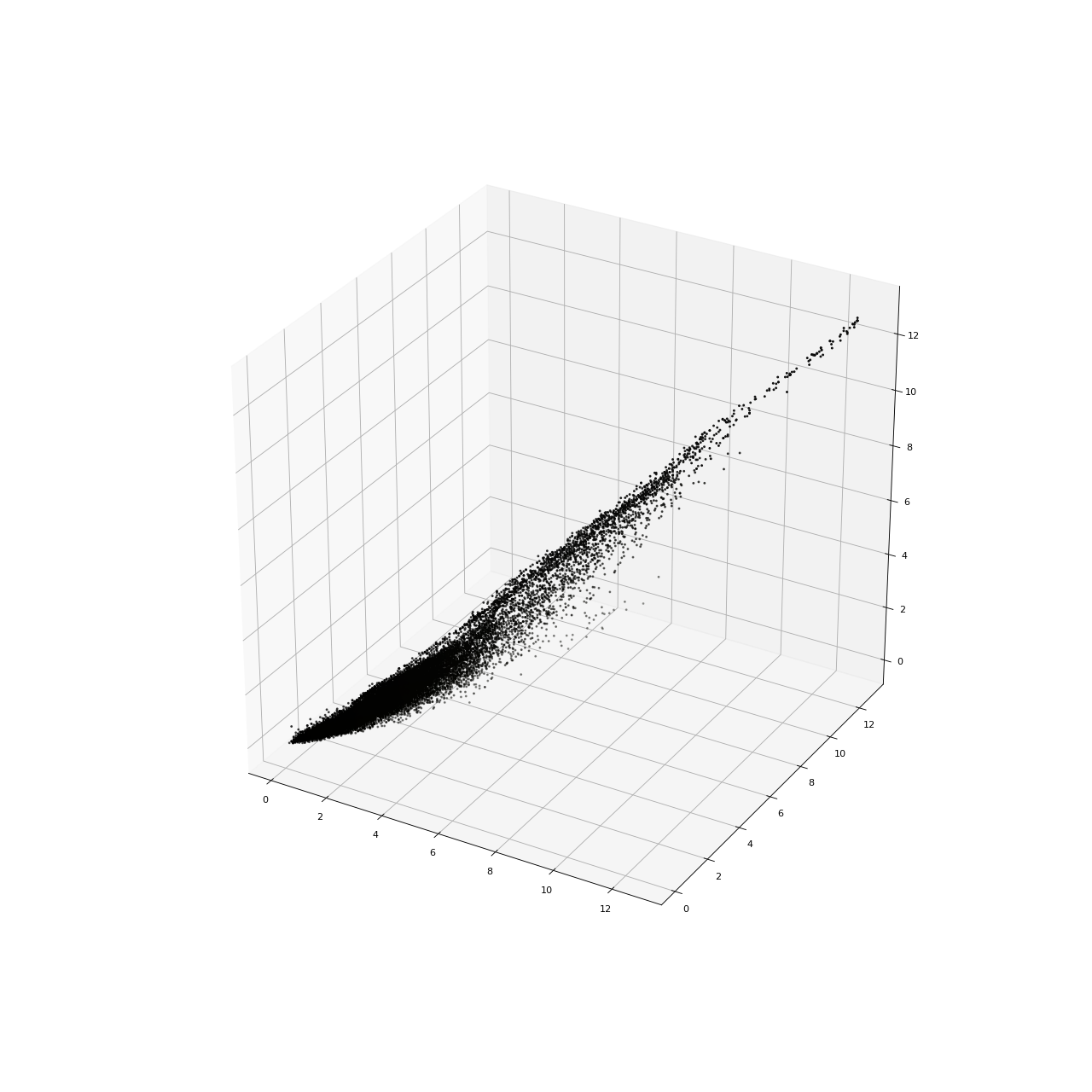

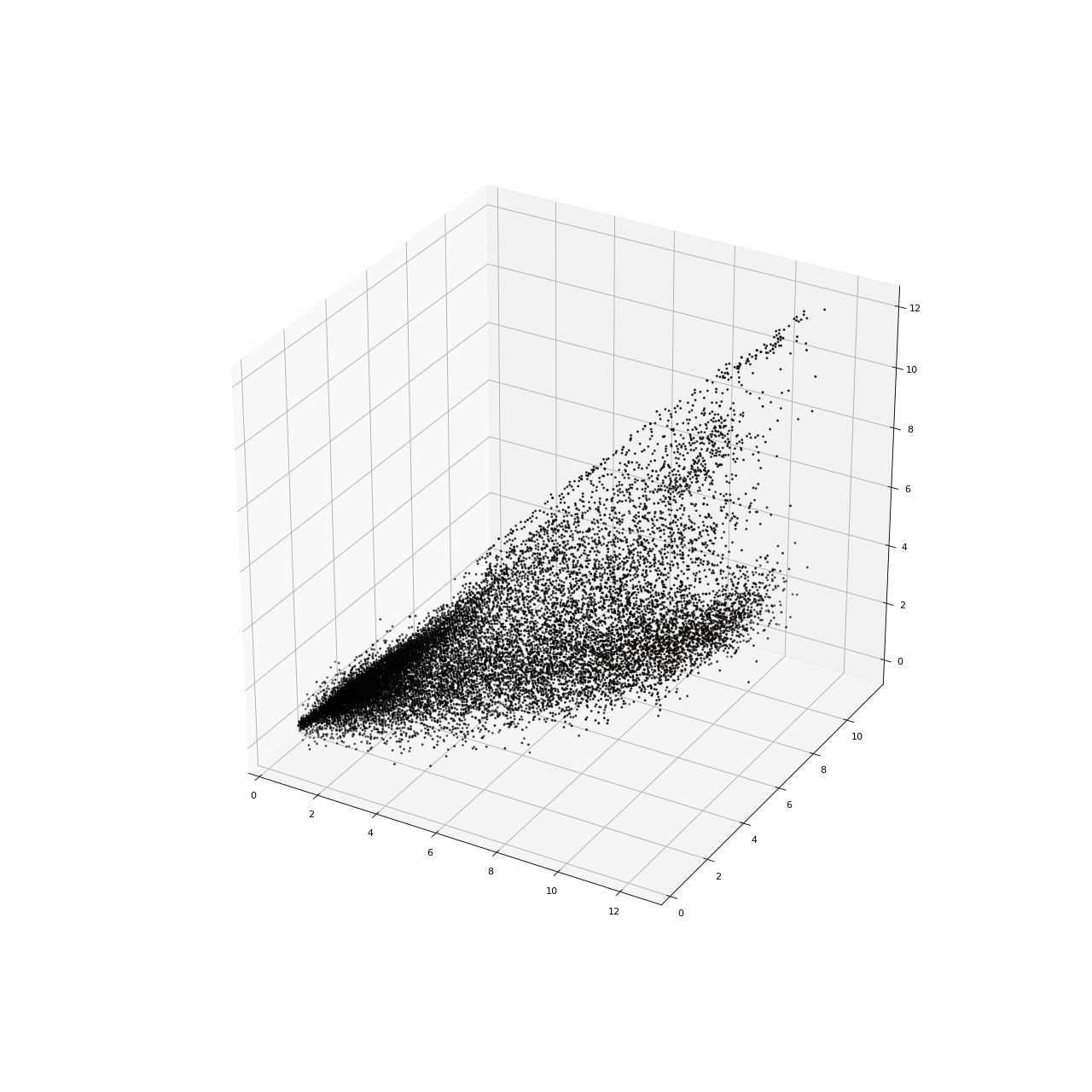


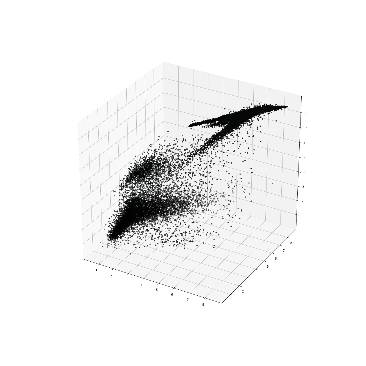

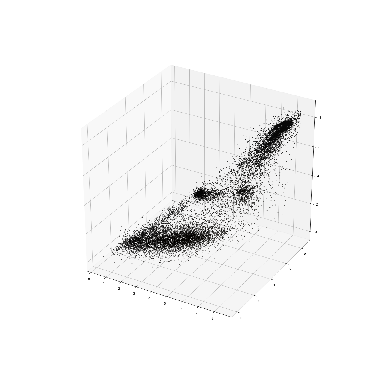


Realistic-1: Two given pictures describe the summer view and autumn view of a forest. We generate the autumn view starting with the summer view and generate the summer view starting with the autumn view. We also show the ground-truth and generated palette distributions in Figure 6.
Realistic-2: In this case the view of West Lake in summer and the view of White Tower in autumn are given, then we aim to do a color transfer and simulate the summer view of White Tower and the autumn view of West Lake, the results are shown in Figure 7, the ground-truth and generated palette distributions are also included.
Realistic-3: We choose MNIST as our data set ( dimensional) and study the Wasserstein mappings as well as geodesic between digit 0 and digit 1, digit 4() and digit 8(), digit 6() and digit 9(). Only partial results are presented in Figure 8 due to space limit.
Training and Results: For realistic-1 and realistic-2 we set the batch size , for realistic-3 in each iteration we take pictures for training, especially for realistic-3 we also add small noise to samples during the training process. From Figure 6 and 7, the generated autumn(summer) views are very close to the true autumn(summer) views, moreover, the similarity between true and generated palette distributions also demonstrate that our algorithm works well in these cases. In realistic-3 we study the Wasserstein geodesic and mappings in original space without any dimension reduction techniques. Our generated handwritten digits follow similar patterns with the ground truth.
5 Conclusion
OT problem has been drawing more attention in machine learning recently. Though many algorithms have been proposed during the past several years for efficient computations, most of them do not consider the Wasserstein geodesics, neither be suitable for estimating optimal transport map with general cost in high dimensions. In this paper we present a novel method to compute Wasserstein geodesic between two given distributions with general convex cost. In particular, we consider the primal-dual scheme of the dynamical OT problem and simplify the scheme via the KKT conditions as well as the geodesic transporting properties. By further introducing preconditioning techniques and bidirectional dynamics into our optimization, we obtain a stable and effective algorithm that is capable of high dimensional computation, which is one of the very first scalable algorithms for directly computing geodesics with general cost, including -. Our method not only computes sample based Wasserstein geodesics, but also provides Wasserstein distance and optimal map. We demonstrate the effectiveness of our scheme through a series of experiments with both low dimensional and high dimensional settings. It is worth noting that our model can be applied not only in machine learning such as image transfer, density estimation, but also in optimal control and robotics, where one needs to study the distribution of mobile agents. We should also be aware of the malicious usage for our method, for instance, it could be potentially used in some activities involving generating misleading data distributions.
References
- Altschuler et al. (2017) Altschuler, J., Niles-Weed, J., and Rigollet, P. Near-linear time approximation algorithms for optimal transport via sinkhorn iteration. Advances in neural information processing systems, pp. 1964–1974, 2017.
- Amos et al. (2017) Amos, B., Xu, L., and Kolter, J. Sinkhorn distances: Lightspeed computation of optimal transport. In International Conference on Machine Learning, pp. 146–155, 2017.
- Arjovsky et al. (2017) Arjovsky, M., Chintala, S., and Bottou, L. Wasserstein gan. In arXiv preprint arXiv:1701.07875, 2017.
- Benamou & Brenier (2000a) Benamou, J. and Brenier, Y. A computational fluid mechanics solution to the monge-kantorovich mass transfer problem. Numerische Mathematik, 84(3):375–393, 2000a.
- Benamou & Brenier (2000b) Benamou, J. and Brenier, Y. A computational fluid mechanics solution to the monge-kantorovich mass transfer problem. In Numerische Mathematik, 2000b.
- Benamou et al. (2010) Benamou, J., Froese, B., and Oberman, A. Two numerical methods for the elliptic monge-ampere equation. ESAIM: Mathematical Modelling and Numerical Analysis, 44(4):737–758, 2010.
- Chen et al. (2016) Chen, Y., Georgiou, T., and Pavon, M. On the relation between optimal transport and schrödinger bridges: A stochastic control viewpoint. In Journal of Optimization Theory and Applications, 2016.
- Chen et al. (2020) Chen, Y., Georgiou, T., and Pavon, M. Optimal transport in systems and control. Annual Review of Control, Robotics, and Autonomous Systems, 4, 2020.
- Courty et al. (2016) Courty, N., Flamary, R., Tuia, D., and Rakotomamonjy, A. Optimal transport for domain adaptation. IEEE transactions on pattern analysis and machine intelligence, 39(9):1853–1865, 2016.
- Cuturi (2013) Cuturi, M. Sinkhorn distances: Lightspeed computation of optimal transport. In Neural Information Processing Systems, 2013.
- Dessein et al. (2018) Dessein, A., Papadakis, N., and Rouas, J. Regularized optimal transport and the rot mover’s distance. The Journal of Machine Learning Research, 19(1):590–642, 2018.
- Dukler et al. (2019) Dukler, Y., Li, W., Tong Lin, A., and Montúfar, G. Wasserstein of wasserstein loss for learning generative models. 2019.
- Fan et al. (2020) Fan, J., Taghvaei, A., and Chen, Y. Scalable computations of wasserstein barycenter via input convex neural networks. arXiv preprint arXiv:2007.04462, 2020.
- Finlay et al. (2020a) Finlay, C., Gerolin, A., Oberman, A., and Pooladian, A. Learning normalizing flows from entropy-kantorovich potentials. In arXiv preprint arXiv:2006.06033, 2020a.
- Finlay et al. (2020b) Finlay, C., Jacobsen, J.-H., Nurbekyan, L., and Oberman, A. M. How to train your neural ode: the world of jacobian and kinetic regularization. In arXiv preprint arXiv:2002.02798, 2020b.
- Flamary et al. (2014) Flamary, R., Courty, N., Rakotomamonjy, A., and Tuia, D. Optimal transport with laplacian regularization. In Advances in Neural Information Processing Systems, Workshop on Optimal Transport and Machine Learning, 2014.
- Flamary et al. (2021) Flamary, R., Courty, N., Gramfort, A., Alaya, M. Z., Boisbunon, A., Chambon, S., Chapel, L., Corenflos, A., Fatras, K., Fournier, N., Gautheron, L., Gayraud, N. T., Janati, H., Rakotomamonjy, A., Redko, I., Rolet, A., Schutz, A., Seguy, V., Sutherland, D. J., Tavenard, R., Tong, A., and Vayer, T. Pot: Python optimal transport. Journal of Machine Learning Research, 22(78):1–8, 2021. URL http://jmlr.org/papers/v22/20-451.html.
- Gangbo et al. (2019) Gangbo, W., Li, W., Osher, S., and Puthawala, M. Unnormalized optimal transport. Journal of Computational Physics, 399:108940, 2019.
- Genevay et al. (2016) Genevay, A., Cuturi, M., Peyré, G., and Bach, F. Stochastic optimization for large-scale optimal transport. In Advances in neural information processing systems, pp. 3440–3448, 2016.
- Genevay et al. (2018) Genevay, A., Peyré, G., and Cuturi, M. Learning generative models with sinkhorn divergences. International Conference on Artificial Intelligence and Statistics, pp. 1608–1617, 2018.
- Grathwohl et al. (2018) Grathwohl, W., Chen, R., Bettencourt, J., Sutskever, I., and Duvenaud, D. Ffjord: Free-form continuous dynamics for scalable reversible generative models. In arXiv preprint arXiv:1810.01367, 2018.
- Gulrajani et al. (2017) Gulrajani, I., Ahmed, F., Arjovsky, M., Dumoulin, V., and Courville, A. C. Improved training of wasserstein gans. In Neural Information Processing Systems, 2017.
- Inoue et al. (2020) Inoue, D., Ito, Y., and Yoshida, H. Optimal transport-based coverage control for swarm robot systems: Generalization of the voronoi tessellation-based method. IEEE Control Systems Letters, 5(4):1483–1488, 2020.
- Kingma & Ba (2014) Kingma, D. P. and Ba, J. Adam: A method for stochastic optimization, 2014.
- Korotin et al. (2019) Korotin, A., Egiazarian, V., Asadulaev, A., Safin, A., and Burnaev, E. Wasserstein-2 generative networks. arXiv preprint arXiv:1909.13082, 2019.
- Krishnan & Martínez (2018) Krishnan, V. and Martínez, S. Distributed optimal transport for the deployment of swarms. IEEE Conference on Decision and Control (CDC), pp. 4583–4588, 2018.
- Kuang & Tabak (2019) Kuang, M. and Tabak, E. Sample‐based optimal transport and barycenter problems. Communications on Pure and Applied Mathematics, 72(8):1581–1630, 2019.
- Kuang & Tabak (2017) Kuang, M. and Tabak, E. G. Preconditioning of optimal transport. SIAM Journal on Scientific Computing, 39(4):A1793–A1810, 2017.
- Kuhn & Tucker (1951) Kuhn, H. W. and Tucker, A. W. Nonlinear programming. In Proceedings of the Second Berkeley Symposium on Mathematical Statistics and Probability, pp. 481–492, Berkeley, Calif., 1951. University of California Press. URL https://projecteuclid.org/euclid.bsmsp/1200500249.
- Lecun et al. (1998) Lecun, Y., Bottou, L., Bengio, Y., and Haffner, P. Gradient-based learning applied to document recognition. Proceedings of the IEEE, 86(11):2278–2324, 1998. doi: 10.1109/5.726791.
- Li et al. (2019) Li, R., Ye, X., Zhou, H., and Zha, H. Learning to match via inverse optimal transport. In J. Mach. Learn. Res., pp. 20, pp.80–1, 2019.
- Li et al. (2018) Li, W., Ryu, E., Osher, S., Yin, W., and Gangbo, W. A parallel method for earth mover’s distance. Journal of Scientific Computing, 75(1):182–197, 2018.
- Lin et al. (2020) Lin, A., Fung, S., Li, W., Nurbekyan, L., and Osher, S. Apac-net: Alternating the population and agent control via two neural networks to solve high-dimensional stochastic mean field games. In arXiv preprint arXiv:2002.10113, 2020.
- Ma et al. (2020) Ma, S., Liu, S., Zha, H., and Zhou, H. Learning stochastic behaviour of aggregate data. In arXiv preprint arXiv:2002.03513, 2020.
- Makkuva et al. (2020) Makkuva, A.and Taghvaei, A., Oh, S., and Lee, J. Optimal transport mapping via input convex neural networks. In International Conference on Machine Learning, pp. 6672–6681, 2020.
- Miyato et al. (2018) Miyato, T., Kataoka, T., Koyama, M., and Yoshida, Y. Spectral normalization for generative adversarial networks. arXiv preprint arXiv:1802.05957, 2018.
- Muzellec et al. (2017) Muzellec, B., Nock, R., Patrini, G., and Nielsen, F. Tsallis regularized optimal transport and ecological inference. In Proceedings of the AAAI Conference on Artificial Intelligence, 31(1), 2017.
- Reinhard et al. (2001) Reinhard, E., Ashikhmin, M., Gooch, B., and Shirley, P. Color transfer between images. IEEE Comput. Graph. Appl., 21(5):34–41, September 2001. ISSN 0272-1716. doi: 10.1109/38.946629. URL https://doi.org/10.1109/38.946629.
- Ruthotto et al. (2020) Ruthotto, L., Osher, S. J., Li, W., Nurbekyan, L., and Fung, S. W. A machine learning framework for solving high-dimensional mean field game and mean field control problems. Proceedings of the National Academy of Sciences, 117(17):9183–9193, 2020.
- Seguy et al. (2017) Seguy, V., Damodaran, B., Flamary, R., Courty, N., R., A., and Blondel, M. Large-scale optimal transport and mapping estimation. arXiv preprint arXiv:1711.02283, 2017.
- Tolstikhin et al. (2017) Tolstikhin, I., Bousquet, O., Gelly, S., and Schoelkopf, B. Wasserstein auto-encoders. In arXiv preprint arXiv:1711.01558, pp. 3440–3448, 2017.
- Tong Lin et al. (2018) Tong Lin, A., Li, W., Osher, S., and Montúfar, G. Wasserstein proximal of gans. 2018.
- Trigila & Tabak (2016) Trigila, G. and Tabak, E. Data‐driven optimal transport. Communications on Pure and Applied Mathematics, 69(4):613–648, 2016.
- Villani (2003) Villani, C. Topics in optimal transportation. Number 58. American Mathematical Soc., 2003.
- Villani (2008) Villani, C. Optimal transport: old and new, volume 338. Springer Science & Business Media, 2008.
- Xie et al. (2019) Xie, Y., Chen, M., Jiang, H., Zhao, T., and Zha, H. On scalable and efficient computation of large scale optimal transport. In In International Conference on Machine Learning, pp. 6882–6892, 2019.
- Xie et al. (2020) Xie, Y., Wang, X., Wang, R., and Zha, H. A fast proximal point method for computing exact wasserstein distance. In Uncertainty in Artificial Intelligence, pp. 433–453, 2020.
- Yang (2020) Yang, I. Wasserstein distributionally robust stochastic control: A data-driven approach. IEEE Transactions on Automatic Control, 2020.
- Yang & Karniadakis (2019) Yang, L. and Karniadakis, G. Potential flow generator with optimal transport regularity for generative models. In arXiv preprint arXiv:1908.11462, 2019.
Appendix A Algorithm
A.1 Preconditioning technique for 2-Wasserstein case
It’s worth mentioning that we can apply preconditioning technique under the 2-Wasserstein cases, i.e., . When the support of distributions and are far away from each other, the computational process might get much more sensitive with respect to vector field . In order to deal with this situation, we consider preconditioning to our initial distribution . In our implementation, we treat as our preconditioning map. We fix its structure as with . Such preconditioning process can be treated as an operation aiming at relocating and rescaling the initial distribution so that the support of matches with the support of in a better way, which in turn facilitates the training process of our OT problem. A similar technique is also carried out by Kuang & Tabak 2017.
Let us denote the optimal vector field of OT problem between and as , then for the vector field , the following theorem guarantees the optimality of .
Theorem 3.
This theorem indicates that our constructed is exactly the optimal transport field for the original OT problem from to . The proof is in Appendix C.
Our computation procedure is summarized in Algorithm 1. We set and as fully connected neural networks and optimize over their parameters.
Remark 2.
In Algorithm 1, we need to sample points from the distribution . To achieve this, we first sample from . Then are our desired samples from .
In Algorithm 1 we define
Appendix B Proof of Theorem 2
Let us denote as the transporting vector field. Recall that we are computing for the Wasserstein geodesic interpolating and . We denote . Then we introduce the following functional of and :
| (24) |
As mentioned in (22), our numerical method is to solve the following saddle point problem
| (25) |
As stated in Theorem 2, the optimal solution obtained from dynamical OT problem (Brenier-Benamou formulation) (7) is a critical point to the functional . Before we prove this result, we need the following lemmas:
Lemma 1.
Given a distribution with density defined on , consider vector field . Define time-varying density as . Suppose for a given , is integrable on . Then
Proof.
We have
∎
Lemma 2.
Suppose is solved from (10) in the paper with initial condition , we further assume . Then we have
| (26) |
Proof.
Now consider Hamilton-Jacobi equation of (10) in the paper:
We take gradient with respect to on both sides, we have
| (27) |
Let us denote for simplicity. We now compute
By plugging into (27), we are able to verify . Thus
| (28) |
Recall defined in the paper, we can verify that . Thus (28) leads to
∎
Lemma 3.
Suppose is solved from (10) in the paper with initial condition , we further assume . Now denote . Then solves
Proof.
Lemma 4.
Suppose is solved from (10) in the paper with initial condition , then
| (31) |
Proof.
Consider particle dynamical OT with its optimal solution as stated in (11) in the paper. Recall Theorem 1 stating that the optimal plan is transporting each particle along straight lines with constant velocity , i.e. for any . Combining these, we have
Notice that we require . This will lead to (31). ∎
Theorem 2.
Recall the solution to the equation system (10) in the paper is and , suppose . Denote , then is a critical point to the functional , i.e.,
Furthermore, .
Proof.
Since we have assumed , we restrict our as well.
We first rewrite by using integration by parts as:
| (32) |
By Lemma 1, (32) can be written as
| (33) | ||||
Now based on (33) here, we are able to compute as
| (34) | ||||
Now we plug , into (34), by Lemma 2, we have
| (35) |
Then using (35) and recall that , one can verify that , similarly, for , we have for all . Thus and we are able to verify .
Appendix C Proof of Theorem 3
Theorem 3.
Appendix D Complete Geodesics in Experiments
D.1 Synthetic Data
Syn-1:


Syn-2: Wasserstein-1.5


Syn-2: Wasserstein-2


Syn-3:


Syn-4:


D.2 Realistic Data
Real-1:


Real-2:
Real-3:


