Longest minimal length partitions
Abstract
This article provides numerical evidence that under volume constraint the ball is the set which maximizes the perimeter of the least-perimeter partition into cells with prescribed areas. We introduce a numerical maximization algorithm which performs multiple optimizations steps at each iteration to approximate minimal partitions. Using these partitions we compute perturbations of the domain which increase the minimal perimeter. The initialization of the optimal partitioning algorithm uses capacity-constrained Voronoi diagrams. A new algorithm is proposed to identify such diagrams, by computing the gradients of areas and perimeters for the Voronoi cells with respect to the Voronoi points.
1 Introduction
In [18] the authors answer a question raised by Polya in [38] and prove that among planar convex sets of given area the disk maximizes the length of the shortest area-bisecting curve. Denote by an open, connected region with Lipschitz boundary. Consider and denote with the usual Lebesgue measure (area in 2D, volume in 3D). Given and , define the shortest fence set to be
| (1) |
In other words, is one subset which minimizes the relative perimeter when the measure is fixed to . In the following, the relative perimeter of is denoted by
| (2) |
In the literature the mapping is sometimes called the isoperimetric profile of the set . The paper [18] cited above solves the problem of maximizing with respect to ,
| (3) |
in dimension two for . In the following denotes the volume of the unit ball in . The choice of the volume constraint does not reduce the generality of the problem, since changing this constant only rescales the solution via a homothety. Classical details regarding the existence of the sets and the definition of the relative perimeter are recalled in the next section.
This work was initiated by the note [29] published on the French CNRS website Images des mathématiques, where it is asked what happens to the solution of (3) when the parameter varies in . This conjecture is attributed to Wichiramala [45] and the article [36] on F. Morgan’s blog presents an extensive discussion regarding the history of the problem. The conjecture was partially solved in dimension two in the following works:
- •
In [5] the authors prove the conjecture in the plane for small fraction areas. The article contains many interesting results related to relative isoperimetric sets.
- •
In [44] the authors prove the conjecture in the plane for domains symmetric with respect to both coordinate axes and perturbations of the unit disk.
Therefore the conjecture remains unanswered for large fraction areas, except for the case . Moreover, other generalizations of this problem can be investigated. It is possible, for instance, to consider the analogue problem in the case of partitions of shortest total boundary measure. Given and consider to be a partition of , in the sense that the union of , is and . Given a vector with consider the shortest partition of with volume constraints to be
| (4) |
In the following we define the isoperimetric profile of a partition given by the constraints by
| (5) |
In other words is the minimal total relative perimeter of a partition with volume constraints given by . Now it is possible to formulate the problem
| (6) |
where the total relative perimeter of the shortest partition with constraints is maximized when has fixed volume. It is obvious that (3) is a particular case of (6) by considering and .
In this paper, problems (3) and (6) are investigated from both numerical and theoretical points of view. In order to approximate solutions of these problems multiple issues need to be addressed:
- •
Compute reliably a numerical approximation of the shortest partition once the domain and the constraints vector are given. It is important to avoid local minimizers at this stage, since the objective is to maximize the shortest perimeter. Any local minimizer may give a false candidate for the solutions of (3) or (6). There are many works in the literature which deal with the investigation of minimal length partitions. In [14] Cox and Flikkema use the surface Evolver software to approximate minimal partitions. In this work the approach presented in [37] is used, where the perimeter is approximated using a -convergence result of Modica and Mortola [34]. This allows us to work with density functions rather than sets of finite perimeter and simplifies the handling of the partition condition. Moreover, working with densities directly allows changes in the topology of the partitions.
Given a domain , a mesh is constructed and finite elements are used in FreeFEM [25] in order to approximate or . When dealing with partitions, in order to accelerate the convergence, an initialization based on Voronoi diagrams with prescribed areas is used.
- •
- •
The family of star-shaped domains (which includes convex shapes) is parametrized using radial functions. Moreover, radial functions are discretized by considering truncations of the associated Fourier series. Using the shape derivative it is possible to compute the gradient of the objective function with respect to the discretization parameters. Once the gradient is known, an optimization algorithm is used in order to search for solutions of (3) and (6). The choice of the optimization algorithm is also an important factor since the computation of is highly sensitive to local minima. Moreover, when changing following a perturbation field found using a shape derivative argument, the configuration of the optimal partition might change. The chosen algorithm is a gradient flow with variable step size.
Minimal length partitioning algorithms presented in [37] or [6] use random initializations. While this illustrates the flexibility of Modica-Mortola type algorithms and the ability of the algorithm to avoid many local minima, choosing random initializations leads to longer computation times required for the optimization algorithm. A classical idea is to use Voronoi diagrams as initializations. However, these Voronoi diagrams should consist of cells which verify the area constraints . In the literature, the notion of capacity-constrained Voronoi diagrams is employed and results in this direction can be found in [4], [3] and [46]. In this work we propose a new way of computing capacity-constrained Voronoi diagrams by explicitly computing the gradients of the areas of the Voronoi cells with respect to variations in the Voronoi points. The gradient of the perimeters of the Voronoi cells is also computed, which allows the search of capacity-constrained Voronoi diagrams with minimal length.
The numerical simulations give rise to the following conjectures:
- •
The result of the convex isoperimetric conjecture seems to generalize to every volume fraction in dimensions two and three.
- •
The same result seems to hold in the case of partitions. For and with arbitrary, the solution of (6) is the disk in 2D and the ball in 3D. It is surprising that this result seems to hold even when the area constraints of the cells of the partition are not the same.
Outline and summary of results. Section 2 presents classical theoretical results regarding approximations of minimal perimeter partitions by -convergence.
Section 3.1 recalls basic aspects regarding the numerical computation of minimal length partitions. Section 3.3 presents the computation of the gradients of the areas and perimeters of Voronoi cells and shows how to use prescribed-area Voronoi cells in order to construct initializations for our optimization algorithm. Section 3.4 presents the computation of an ascent direction for the shape optimization algorithm using the notion of shape derivative. The choice of the discretization and the optimization algorithm for approximating solutions of problems (3) and (6) are presented in Section 3.5. We underline that the maximization algorithm approximates solutions to a max-min problem, and the optimal partitioning algorithm presented in Section 3.1 is run at every iteration.
Finally, results of the optimization algorithm in dimensions two and three are presented in Section 4. The numerical results suggest that the solution of problems (3) and (6) is the disk in dimension two and the ball in dimension three. A brief discussion of the optimality conditions is presented in Section 5.
2 Theoretical aspects
2.1 Minimal relative perimeter sets and partitions
The appropriate framework to work with sets of finite relative perimeter in is to consider the space of functions with bounded variation on
where
As usual represents the space of functions defined on with compact support in . Using the divergence theorem it is easy to observe that if is of class then
If is a subset of its generalized perimeter is defined by , where represents the characteristic function of . All these aspects are classical and can be found, for example, in [2, 8].
The fact that problems (1) and (4) have solutions is classical and is a consequence of the fact that the generalized perimeter defined above is lower-semicontinuous for the convergence of characteristic functions. For more aspects related to solutions of these problems see [32, Chapter 17]. The book previously referenced also presents aspects related to the regularity of optimal partitions in Part Four. Aspects about optimal partitions in the smooth case are presented in [35] where qualitative properties of minimal partitions in the plane and on surfaces are presented.
Proving existence of solutions for problems (3) and (6) is more difficult since these are maximum problems and the perimeter is lower semicontinuous. We recall that problem (3) was solved in [18] in the case , . In particular, existence was proved exploiting results in [13] which show that in this case the minimal relative perimeter sets are convex. In the following we prove that solutions exist in the class of convex domains for arbitrary area constraints.
Theorem 2.1.
Problem (3) has solutions in the class of convex sets, i.e. given there exist convex sets which maximize among convex sets with fixed volume .
Proof: We divide the proof into steps which allow us to apply classical methods in calculus of variations.
Step 1: Upper bounds. In the following denote by the minimal measure of the projection of on a hyperplane (in dimension two this corresponds to the minimal width). For convex bodies the following reverse Loomis-Whitney inequality holds true:
where the minimum is taken over all orthonormal bases of and represents the projection of onto a hyperplane orthogonal to . In [30] it is shown that there exists a constant such that . In particular, this shows that the minimal projection verifies . As a direct consequence is bounded above in the class of convex sets which satisfy .
It is immediate to see that the quantity gives an upper bound for . To justify this choose the direction for which is minimal and slice with a hyperplane orthogonal to which divides into two regions and with volume . The relative perimeter of the set in is at most equal to , the measure of the projection. Therefore, we may conclude that in the class of convex sets with measure the quantity is bounded from above, and the upper bound only depends on and . This implies the existence of a maximizing sequence which verifies and , where the supremum is taken in the class of convex sets.
Step 2: Compactness. When dealing with a sequence of convex sets we may extract a subsequence converging in the Hausdorff distance provided the sets are uniformly bounded. For classical aspects related to the Hausdorff distance we refer to [26, Chapter 2]. Therefore, in the following we show that the diameters of convex sets forming the maximizing sequence are uniformly bounded.
First, let us note that since is a maximizing sequence for there exists a positive constant such that . Since we also have for . The results in [20] show that the minimal perimeter projection, the diameter and the volume of a convex set satisfy
It is now immediate to see that , and therefore the diameters of are bounded. Without loss of generality we may assume that are contained in a large enough ball. Applying the classical Blaschke selection theorem we find that there exists a maximizing sequence, denoted for simplicity by , such that converges, with respect to the Hausdorff distance, to the convex set . Moreover, the volume is continuous for the Hausdorff distance among bounded convex sets, so also satisfies the volume constraint .
Step 3. Continuity. The last step is to prove that is indeed equal to . This is a direct consequence of [40, Theorem 4.1], which states that if is a sequence of convex bodies in and in the Hausdorff distance then for every . This finishes the proof as the limit is indeed a maximizer for (3).
Remark 2.2.
Removing the convexity assumption is not straightforward. Nevertheless, using the regularity results regarding solutions of (1) it is possible that this result could be partially extended in the general case. There are multiple difficulties which follow the structure of the proof above:
- •
Proving there exists an upper bound in (3).
- •
Proving that a maximizing sequence is bounded: long tails may not intersect the minimizing set in (1) therefore cutting them may increase .
- •
Obtaining compactness results of a maximizing sequence: classically this should be possible when working in the class of sets of finite perimeter.
- •
Proving that the maximizing sequence converges to an actual maximizer. This would involve obtaining some continuity properties regarding the perimeter of a sequence of sets. This is not straightforward, as the perimeter is only lower-semicontinuous for the convergence of characteristic functions. Nevertheless, using the regularity of minimal relative perimeter sets might help obtain the desired results.
The case of partitions can be handled using a similar strategy in the class of convex sets. The missing ingredient is the convergence of the minimal perimeters of partitions, analogue to the results in [40].
Theorem 2.3.
Problem (6) has solutions in the class of convex sets, i.e. given there exist convex sets which maximize among convex sets with fixed volume .
Proof: As in the proof of Theorem 2.1 it is straightforward to give upper bounds for in terms of (the minimal measure of the projection on a hyperplane). A maximizing sequence would have a positive lower bound for the sequence of minimal projections on hyperplanes. Therefore the diameters of are bounded from above and we may assume that the convex sets converge to a convex set (with respect to the Hausdorff distance). The set also verifies the volume constraint .
It only remains to prove the continuity of the minimal partition perimeters for the convergence with respect to the Hausdorff distance. In order to do this, the same tools as in the proof of Theorem 4.1 in [40] can be used.
- 1.
Lower-semicontinuity. Theorem 3.4 in [40] shows that there exist bilipschitz maps with Lipschitz constants converging to , the Lipschitz constants of the inverse maps also converging to . The volumes and perimeters of the images of finite perimeter sets have upper and lower bounds as follows:
Let be a minimal perimeter partition for with constraint . Then is a partition of with . Extracting a diagonal sequence, we may assume that converges with respect to the Hausdorff distance to a partition of as . Using the estimates above and the fact that the perimeter is lower semi-continuous with respect to the convergence of finite perimeter sets we have
- 2.
Upper-semicontinuity. It remains to prove that . Reasoning by contradiction, suppose that . Up to a subsequence we may assume that converges. Choose a minimal partition in with constraints . As in [40] using these sets it is possible to construct better competitors on some for large than the corresponding optimal partition. This leads to a contradiction.
Indeed, forms a partition of , which may fail to satisfy the volume constraints. Optimality conditions imply that common boundaries of the sets in the partition are regular hypersurfaces. Therefore, it is possible to perturb these boundaries around regular points in order to attain the desired volume constraints. Moreover, for large enough this will produce partitions which verify
contradicting the optimality of .
This concludes the proof of the existence of solutions for the given problem.
Remark 2.4.
Existence results obtained in this section may also be generalized to the case of manifolds, in particular when is the boundary of a convex set in . There exist sets which are surfaces of co-dimension that are boundaries of some convex set in and have fixed measure which maximize the minimal relative geodesic perimeter of a subset or partition with given measure constraints.
2.2 Relaxation of the perimeter - Gamma convergence
A key point in our approach is to approximate minimal length partitions . In order to avoid difficulties related to the treatment of the partition constraint it is convenient to represent each set in the partition as a density . Then, the partition constraint can be simply expressed by the algebraic equality on . The next aspect is to approximate the perimeter of a set represented via its density function. A well known technique is to use a -convergence relaxation for the perimeter inspired by a result of Modica and Mortola [34]. The main idea is to replace the perimeter with a functional that, when minimized, yields minimizers converging to those that minimize the perimeter.
Let us briefly recall the concept of -convergence and the property that motivates its use when dealing with numerical optimization.
Remark 2.5.
Let be a metric space. For consider the functionals . We say that -converges to and we denote if the following two properties hold:
- (LI)
For every and every with we have
(7) - (LS)
For every there exists such that and
(8)
An important consequence is the following classical result concerning the convergence of minimizers of a sequence of functionals that converge.
Proposition 2.6.
Suppose that and minimizes on . Then every limit point of is a minimizer for on .
Therefore, in practice, in order to approximate the minimizers of it is possible to search for minimizers of , for small enough.
Let us now state the two theoretical results that are used in this work concerning the -convergence relaxation of the perimeter and of the total perimeter of a partition, with integral constraints on the densities. The first result is the classical Modica-Mortola theorem [34]. Various proofs can be found in [1, 8, 11]. In the following is a bounded, Lipschitz open set. Consider a double well potential which verifies the following assumptions: is of class , if and only if and has exactly three critical points. For such a double well potential described previously, denote . In the following represents the fraction used for the volume constraint.
Theorem 2.7 (Modica-Mortola).
Define by
and
Then in the topology.
In [37] this result was generalized to the case of partitions and was used to compute approximations for . For with , in order to simplify notations, let us denote by the space of admissible densities which verify the integral constraints and the algebraic non-overlapping constraint
The -convergence result in the case of partitions is recalled below.
Theorem 2.8.
Define by
Then in the topology.
A proof of this result can be found in [37]. In the numerical simulations the double well potential is chosen to be which gives the factor in the results shown above.
Remark 2.9.
It can be seen that corresponds to a density that is a minimizer of in Theorem 2.7. Moreover, corresponds to a family of densities which minimizes in Theorem 2.8. Using the result recalled in Proposition 2.6 it is possible to approximate these minimizers by those of and , respectively, for small enough. From a numerical point of view, dealing with the minimization of and is easier since the variable densities are regular.
Remark 2.10.
The structures of minimizers of was widely studied in the literature as can be seen in the papers [23], [31], [42]. It can immediately be seen that, assuming is at least of class , minimizers of verify an optimality condition of the form
| (9) |
where is a Lagrange multiplier for the volume constraint. Classical regularity theory results that can be found in [21] allow us to employ a bootstrap argument and conclude that is of class in the interior of and has the regularity of up to the boundary. For example, for smooth domains the optimizer is also smooth up to the boundary of . Moreover, it can be proved that the minimizer takes values in . In the case when is convex results found in [22, Chapter 3] show that solutions of the above problem are in .
The same type of results hold for minimizers of in the case of partitions, with eventual singularities at junction points between three or more phases in the partition. Nevertheless, the contact between the optimal partition and the boundary has the desired regularity.
Remark 2.11.
The results in [31] show that the Lagrange multiplier for the volume constraint in (9) has a geometric interpretation. Given a volume fraction , as , the Lagrange multiplicator converges to times the mean curvature of the shortest fence set , where was defined before Theorem 2.7. Recall that this minimal set , being optimal for the relative perimeter under a volume constraint has constant mean curvature inside . Moreover, as shown in [42], taking as a test function in (9) gives an explicit formula for the Lagrange multiplier
| (10) |
Since in the numerical section we deal with the minimization of for fixed , we briefly recall existence results related to these problems. In the following we suppose that the double well potential is Lipschitz continuous on . This is not restrictive since minimizers of are densities which take values in , which means that values of far away from this interval do not matter in the analysis.
Theorem 2.12.
(i) Problems
admit solutions for a Lipschitz domain with finite volume. In the following we denote by and the optimal values obtained when minimizing and , respectively.
(ii) Given and problems
admit solutions in the class of convex sets.
Proof: The proof of (i) is classical. Note that the constraints on the density functions are embedded in the definition of the functionals to be minimized. We give the ideas for as is just a particular case. The existence proof goes as follows:
- •
The functional is obviously bounded from below by zero. Moreover, truncating the density functions to take values in does not increase the value of . This allows us from now on to assume that the densities have values in this interval.
- •
Minimizing sequences exist and they are bounded in , which allows us to extract a subsequence weakly converging in . The constraints are stable under the convergence. Moreover, the lower-semicontinuity of the norm and Fatou’s lemma allow us to see that any weak -limit point of the minimizing sequence is a minimizer.
The proof of (ii) follows the same lines as the proofs of Theorems 2.1, 2.3. As in the proof of these theorems, we start by noticing that the minimal measure of the projection of on a hyperplane is bounded from above. We detail the proof for , while the proof in the case of partitions follows the same path. In order to emphasize the dependence of on we write .
Upper bound. Choose the direction for which is minimal and equal to . Given a hyperplane orthogonal to consider the function , where is the signed distance to the hyperplane (choosing an orientation) and are given by
This type of construction is standard when proving the limsup part of the -convergence proof for the Modica-Mortola type results in Theorems 2.7, 2.8 (see for example [33]). The coarea formula and the fact that allows us to write
The definition of and a continuity argument allow us to deduce that there is a position of the hyperplane for which the constraint is verified.
Using the coarea formula to evaluate we obtain
The last inequality comes from the fact that is a slice of orthogonal to and its measure is at most . Moreover, we can restrict the bounds in the one dimensional integral to and since for not in this interval the integrand is zero. A simple computation gives
Thus we obtain
where the last equality comes from the change of variables . This quantity depends only on and and is bounded from above independently of .
Compactness. The same argument used in the proof of Theorem 2.1 can be applied in order to conclude that there exists a maximizing sequence converging in the Hausdorff distance to a convex set with non-empty interior and volume . Moreover, we may assume that there exists a bounded open set such that are contained in .
Following the ideas in [26, Chapter 2] we may assume that and satisfy an -cone condition, or equivalently that they are Lipschitz regular with a uniform Lipschitz constant. In this case, the convergence with respect to the Hausdorff distance implies that .
Continuity. It now remains to prove that as . Let us note first that since is a maximizing sequence we have . Consider a minimizer such that .
Since and have a uniform Lipschitz constant (as recalled above), using the extension theorems recalled in [10, Theorem 3.4], there exists an extension of which verifies . Together with the results recalled in Remark 2.10 we find that . Combining this with the fact that implies that
We cannot conclude yet, since may not satisfy the integral constraints on .
In order to fix this, let be a point in the interior of . For large enough there exists a ball of radius such that . Denote by the function which is equal to the distance to inside and zero outside. We use this function to construct functions , for , which verify the integral constraints . Since
we necessarily have . This immediately shows that
as .
Since we find that . This concludes the proof of the existence result. The case of partitions can be handled in a similar manner with the additional difficulty that the area constraints and sum constraints need to be handled simultaneously. This can be achieved by modifying the candidate densities in a finite family of balls.
3 Numerical modeling
3.1 Numerical framework for approximating minimal perimeter partitions
In this section the numerical minimization of and is discussed. Since is a general domain in this work, we choose to work with finite element discretizations. Given a triangulation of , denote by the set of the nodes. Working with Lagrange finite elements, a piecewise affine function defined on the mesh is written . As usual, are the piece-wise linear functions on each triangle, characterized by . For a finite element function, the values are given by and we denote . With these notations, it is classical to introduce the mass matrix and the rigidity matrix defined by
As an immediate consequence of the linearity of the decompositions , we have that
This immediately shows that the functionals and can be expressed in terms of the mass and rigidity matrices and using the expression
| (11) |
where . The gradient of this expression w.r.t. can be computed and is given by
| (12) |
where denotes pointwise multiplication of two vectors: .
It is obvious that with (11) and (12) it is possible to implement a gradient-based optimization algorithm in order to minimize and . The software FreeFEM [25] is used for constructing the finite element framework and the algorithm LBFGS from the package Nlopt [28] is used for the minimization of (11). We address the question of handling the constraints in the next section.
3.2 Area constraints and projections
The area or volume constraint can be expressed with the aid of the vector with . Indeed, with this notation, for a finite element function we have .
Projection for one phase. Let us start with the projection of one function onto the integral constraint. Given a finite element function and its values at the nodes we search a function with values at nodes verifying the constraint by solving
which leads to .
An alternative way of handling the constraint during the optimization process is to project the initial vector on the constraint and project the gradient onto the hyperplane at each iteration. This can simply be done by using in the relation above. Such a modification of the gradient allows us to use efficient black-box optimization toolboxes, since quasi-Newton algorithms like LBFGS will perform updates based on a number of gradients stored in memory. If these gradients verify , the integral constraint will be preserved throughout the optimization process.
Projection for multiple phases. In the case of partitions projections on the integral constraints were already proposed in [37] (when using finite differences) and in [6] (when using finite elements). A drawback of using orthogonal projections parallel to the vector is the fact that the vector is modified almost everywhere in the domain , which also includes the regions where it is or . As observed in [9], this can cause resulting optimal densities to be non-zero at interfaces between two cells and at triple points. The solution proposed was to use instead projections parallel to . It is possible to note that, using this method, the functions are mainly modified only at the interface of transition between or .
Let us now describe the construction of the projection algorithm on the constraints
with the compatibility condition . Consider and and perform the transformation
in order to satisfy the constraints
| (13) |
and
| (14) |
It is easy to note that:
- •
in view of (14), given we can find :
- •
in view of (13), given we can find using the relations above.
In the following we introduce the quantities . Again, in view of (13), if are known, then are known and so is . In order to obtain a system for , let us note that
With this in mind we get
In order to further simplify the above expression, let’s make the following notations
- •
- •
- •
,
This gives
which can be written in the form with and
One may note that the above system is singular since the sum on the columns of is equal to and therefore
where . This is due to the fact that one of the constraints is redundant, in view of the compatibility condition. In practice we simply discard one unknown and set it to zero.
As noted previously, the same procedure can be applied to the gradients associated to each in order to satisfy at every iteration
This allows us to preserve the constraints when using a black-box LBFGS optimizer when initial parameters satisfy the integral and sum constraints.
3.3 Initializations for 2D partitions - Voronoi diagrams
The optimization algorithm for approximating and is ready to be implemented, following the ideas shown in the previous sections. There is, however, the choice of the initialization which is non-trivial and which has an impact on the performance of the optimization algorithm. It was already noted in [37] and [6] that starting from random initializations is possible, but some additional work needs to be done in order to avoid constant phases, which are encountered at some local minimizers. Keeping in mind that the optimal partition problem needs to be solved multiple times during the optimization algorithm, we propose below a different initialization strategy, based on Voronoi diagrams. The use of Voronoi diagrams for generating initializations is a rather natural idea when dealing with partitions and was already mentioned in [14]. In this section is assumed to be a polygon.
Using random Voronoi diagrams is not very helpful, since area constraints are not verified in general. This led us to consider Voronoi diagrams which verify the area constraints, which in the literature are called capacity-constrained Voronoi diagrams. Algorithms for computing such diagrams were proposed in [4] for the discrete case and in [3] for the continuous case. In the continuous case the method employed in [3] was to optimize the position of one Voronoi point at a time using the gradient-free Nelder-Mead method. In [46] the authors propose efficient ways of generating such diagrams, but for weighted Voronoi diagrams only. In the following we propose an alternative method for constructing capacity-constrained Voronoi diagrams by computing the sensitivity of the areas of the Voronoi cells with respect to the position of the points generating the respective Voronoi diagram. Since we are also interested in minimizing the perimeter, the computation of the sensitivity of the perimeter of Voronoi cells is also described.
Terminology related to Voronoi diagrams. Given a set of points (called Voronoi points) the associated Voronoi diagram consists of Voronoi cells defined for by
Each Voronoi cell is a polygonal region (possibly unbounded). The vertices of are simply called vertices in the following (please observe the difference between the Voronoi points and the Voronoi vertices). The edges of are called ridges, some of which can be unbounded. Each ridge connects two Voronoi vertices (possibly at infinity, for unbounded ridges) called ridge vertices. Moreover, each ridge separates two of the initial points, called ridge points. All structure information of a Voronoi diagram associated to a set of points can be recovered as an output to some freely available software like scipy.spatial.Voronoi. The Voronoi diagrams are not restricted to a bounded domain. It is possible, however, to consider restrictions of a Voronoi diagram to a bounded set by simply intersectiong the regions with the set . In our implementation the intersection of polygons is handled using the Shapely Python package for computational geometry.
In the following, given the points , we consider the Voronoi regions restricted to a finite domain re-defined by . Note that in some cases, some may be void if does not contain the associated point . We explain below how to compute the gradients of the areas and perimeters of with respect to positions of the points .
Gradient of the areas of the Voronoi cells. The derivative of a functional that can be represented as an integral over the Voronoi cell with respect to the Voronoi points can be computed if the normal displacement of the cell is known. This fact was recalled in [17] and [27] and is classical in the shape derivative theory. However, since the functionals considered there were sums over all Voronoi cells , the contributions coming from the variations of the boundary cancelled themselves and only the variation of the integrand mattered.
This is no longer the case in our situation. The area of the voronoi cell is and its directional derivative when perturbing a point in direction is given by the integral on the boundary of the normal variation of : , where is the infintesimal displacement of the boundary of when moving in the direction . More explicitly, if is the Voronoi cell for then , where the vector field is defined by on the boundary of .
For a given ridge with associated ridge points , we perturb the point and investigate the derivative of the normal perturbation of as . The two main perturbations are the following:
- •
is collinear with : in this case the perturbation induced on the ridge is just . (see Figure 2 (left)). The associated infinitesimal normal perturbation is constant equal to .
- •
is orthogonal to : in this case the infinitesimal perturbation induced on the ridge is a rotation around the intersection of and . The associated infinitesimal normal perturbation varies linearly on from to (the signs vary with respect to the orientation of the orthogonal perturbation). (see Figure 2 (middle)). In order to prove this it is enough to consider the normal perturbation of the ridge illustrated in Figure 2 (right) and take the limit as .
For a general perturbation of we denote by the normal vector to pointing outwards to and by the unit vector collinear with . Furthermore, consider the notations for the normal and tangential contributions (computed as one dimensional integrals on of the infinitesimal perturbations described above):
| (15) |
By symmetry, these contributions will be similar, but with changed signs when perturbing with . The contributions to the gradients of the areas of the cells and when perturbing or are described in the table below:
|
|
(16) |
The algorithm for computing the gradient of the areas of the cells simply iterates over all the Voronoi ridges that intersect and for each ridge adds the contributions described in (16).
Algorithm 1 describes the computation of the gradient of the areas of the cells. The coordinates of the input points are given in the vector and the output is the real matrix of size containing as columns the gradients of the areas of the cells with respect to the coordinates.
The explicit formulas for the gradients of the areas allow us to easily find capacity-constrained Voronoi diagrams as results of an optimization algorithm. For given constraints with , it is enough to minimize the functional
| (17) |
In order to obtain more regular structures it is also possible to minimize the energy
| (18) |
under the capacity constraints . The energy (18) is employed for characterizing centroidal Voronoi diagrams where each Voronoi point coincides with the centroid of the cell . In particular, Centroidal Voronoi diagrams are critical points for (18). See [46] for more details regarding this functional. Examples in this sense are shown in Figure 3. The constrained minimization is done using the MMA algorithm [43] from the NLOPT library [28]. Note that all constraints are coded as inequality constraints in this algorithm: . Since form a partition of it is immediate to see that if the sets satisfy the inequality constraints, they, in fact, also satisfy the equality constraints .
Remark 3.1.
It is also possible to generalize the gradient formulas when a density is involved, when dealing with quantities of the type , where is a given density. The shape derivative of is , where is the perturbation of the boundary . The boundary perturbations are obviously the same, but the computations in (15) are no longer explicit, and a one-dimensional numerical integration needs to be performed for each Voronoi ridge.
Gradient of the perimeter of the Voronoi cells. We saw that in order to compute the gradient of the areas of the Voronoi cells, the normal displacement of the Voronoi ridges needed to be understood, when moving the Voronoi points. On the other hand, the variation of the perimeter of a Voronoi region depends on the tangential perturbation of the Voronoi ridges. In order to understand this perturbation one needs to see how the Voronoi vertices move when perturbing the Voronoi points. Moreover, it can be observed that when two Voronoi vertices merge, i.e. a Voronoi ridge collapses, the total perimeter of the cells is not smooth. This behavior is illustrated by an example shown in Figure 4.
Therefore, we suppose in the following that each Voronoi vertex is in contact with at most three Voronoi ridges. Moreover, the definition of the Voronoi cells allows us to conclude that in this situation each Voronoi vertex is the circumcenter of the triangle determined by the three points associated to the neighboring Voronoi regions. This allows us to transform perturbations of the Voronoi points into perturbations of the Voronoi vertices, by looking at the following well known formulas for the circumcenter of a triangle with vertices :
| (19) |
where . The formulas above are well defined as long as the three points are not colinear. Moreover, it is immediate to see that in this case the circumcenter varies smoothly with respect to the coordinates of the vertices of the triangle. The infinitesimal perturbation of the circumcenter when moving can be computed by simply differentiating the above formulas w.r.t. and . Once the derivative of the circumcenter is known, in order to find the gradient of the prerimeter it is enough to project this derivative on all the Voronoi ridges going through the respective circumcenter and add the contribution to the gradient of the perimeter of each cell with respect to the corresponding coordinates. See Figure 5 for more details.
Variations induced by the Voronoi nodes are enough to compute the gradient of perimeters of Voronoi cells that do not intersect the boundary of the bounding polygon. For the boundary cells, it is necessary to describe the perturbation of intersections between Voronoi ridges and the bounding polygon. Fortunately, this can also be described using variations of circumcenters for some particular triangles.
Indeed, let be a Voronoi ridge intersecting a side of the bounding polygon at the point and let be the associated Voronoi points. Consider now the reflection of the point with respect to the line supporting . Then obviously is the circumcenter of the triangle and the variation of with respect to perturbations of can be found using the same procedure as above. See Figure 5 for more details. The algorithm for computing the gradients for the perimeters of the Voronoi cells is presented in Algorithm 2, assuming that every Voronoi vertex is a circumcenter of exactly one triangle determined by the Voronoi points.
Using the gradients for the area and perimeters of Voronoi cells it is possible to perform a constrained minimization of the perimeter under area constraint starting from random Voronoi initializations. The optimization is performed with Nlopt [28] optimization toolbox in Python using the MMA [43] algorithm. Some examples of initializations obtained are shown in Figure 6. The initial Voronoi points are chosen randomly inside the polygon . In order to accelerate the convergence of the optimization algorithm a few iterations of Lloyd’s algorithm are performed before starting the optimization process. Recall that Lloyd’s algorithm consists in replacing the Voronoi points by the centroids of the respective cells iteratively (see for example [46] for more details). In order to deal with local minima multiple optimizations (typically ) are performed for every polygon and the one with the partition having the least perimeter is retained as a valid initialization. Note that the algorithm gives similar topologies with the best known ones shown in [14] for the case of equal areas and in [24] for the case of cells with two different areas.
Initialization of a partition. Having at our disposal the gradients of areas and perimeters of Voronoi cells, we are now ready to propose initialization algorithms for optimal partitioning algorithm. In practice we use one of the options below:
- 1.
Compute minimizers of (17) starting from random Voronoi points . Repeat the procedure a number of times and keep the configuration having the smallest total perimeter. This works well when the areas of the cells are the same.
- 2.
Optimize the total perimeter of the Voronoi cells under capacity constraints starting from random Voronoi points . Repeat the procedure a number of times and keep the configuration having the smallest total perimeter. This approach gives good results when the areas of the cells are different and the optimization process is more difficult, since more local minima are present.
- 3.
When random initializations work very well.
- 4.
In dimension three random initializations were used for and random Voronoi initializations were used for .
3.4 Shape derivative
In order find perturbations of the domain that decrease the value of a functional the concept of shape derivative is used. For a Lipschitz domain , the functional is said to be shape differentiable at if there exists a linear form such that for every vector field we have
where denotes the identity mapping. Classical results from [41, Section 2.31] and [26, Section 5.2] show that for a function that varies smoothly with respect to perturbations of , the functional is shape differentiable with
| (20) |
A nice overview of the basic notions regarding shape derivatives, together with the associated references is given in the paper [12].
We are interested in finding the shape derivatives of and which are minimal values obtained through constrained optimization. In the following we perform these computations assuming that the corresponding shape derivatives exist. Methods used in the following are inspired from the following works:
- •
In [16, Chapter 10, Sections 2.3, 5.4] the shape derivation of a minimum problem and, respectively, a saddle point is described.
- •
In [19, Capter 3] the derivative of the minimal value problem of a constrained problem where the objective and the constraints depend on a parameter is given in the finite dimensional case.
- •
In [7, Chapter 4] the differentiability of the minimal value given by a constrained parametric problem is considered in Banach spaces.
In our case we are in the framework of the derivation of a saddle point. However, we were not able apply the first result cited above to prove rigorously that the shape derivative exists. In the following we use a formal approach in order to identify the formula for the shape derivatives that are of interest for us.
The case of one phase. Consider which minimizes from Theorem 2.7 and suppose that is unique. We assume that varies smoothly with respect to perturbations of the boundary of and that its shape derivative exists and belongs to . Remark 2.10 underlines the fact that is in the interior of and has the regularity of up to the boundary. In the following we suppose that convex (or, in general, at least of class ), which implies that is indeed in and the gradient has a well defined trace on . The function has the same structure as in (20). Using the classical chain rule for the shape derivatives (see for example [12, Lemma 26]) we obtain that
| (21) |
where is the shape derivative of with respect to .
Recall (see Remark 2.10) that minimizing under the constraint implies the existence of a Lagrange multiplier such that
for every . Taking in the previous equation gives
| (22) |
Recall that also verifies the constraint . Differentiating this with respect to the shape gives
| (23) |
Combining (21), (22) and (23) gives
| (24) |
The previous formula corresponds to the shape derivative of the Lagrangian
with respect to the shape when and . This is in accord with similar results in [16, Chapter 10, Section 5.4], [7, Chapter 4] and [19, Chapter 3].
Note that the formula (24) does give a valuable and reasonable assumption on the perturbation of the boundary that increases the length of the set having minimal perimeter. Notice that the term is non-zero (and strictly positive) only in the neighborhood of the contact points of the minimal relative perimeter set with the boundary . Moving the boundary outwards at these points with a small enough step size will increase the minimal perimeter .
On the other hand the term containing models the movement of the relative isoperimetric set when the boundary of is perturbed away from the contact points. Indeed, recall that and the Lagrange multiplier is proportional (as ) to the curvature of the isoperimetric set , as shown in Remark 10. Therefore, when perturbing away from the contact points with the inner boundary of is pulled in one direction or another (corresponding to the change in the volume) and the corresponding variation of the minimal perimeter is given by the mean curvature of the isoperimetric set.
In the case the solution is not unique, we cannot assume that varies smoothly with . Indeed, perturbing the boundary of with the normal velocity given by may drastically change the topology of the minimal set. Nevertheless, perturbing the boundary of with this normal velocity will eventually increase the value of . In Figure 7 the numerical approximation of is shown together with the values of . Perturbing in the normal direction as shown will increase the minimal value, provided the solution is unique. It can be noted that the term is dominant in the shape derivative, as the second term is of order . Recall that the results given in [31] show that the the Lagrange multiplier as a bounded limit as , proportional to the constant mean curvature of the limiting minimal interface.
Remark 3.2.
Multiple approaches may exist in order to make the above computation a rigorous proof of the shape derivative formula and we describe a few below. The technical difficulties involved do not allow us to present such a complete proof.
- •
In [16, Chapter 9, Theorem 5.1] a method that computes the directional derivative of a saddle point is described. However, it is not clear if this result applies to our case. On the other hand, one may note that this method would give the same result as the formal method described previously.
- •
The computation shown above strongly depends on the existence of the shape derivative . The existence of this derivative is not obvious even under the assumption that is a unique minimizer. It may be possible to apply techniques similar to those in [26, Section 5.7] or [41, Section 2.29] in order to deduce that the unique minimizer is differentiable with respect to the shape .
Remark 3.3.
The hypothesis regarding the uniqueness of for the shape derivative to exist is similar to the hypothesis needed when differentiating the eigenvalue of an operator with respect to the shape. When dealing with multiple eigenvalues, the shape derivative does not exist, but directional derivatives are available. For more details see [26, Chapter 5]. It is possible that such theoretical results could be obtained in our case, but this goes outside the scope of this article.
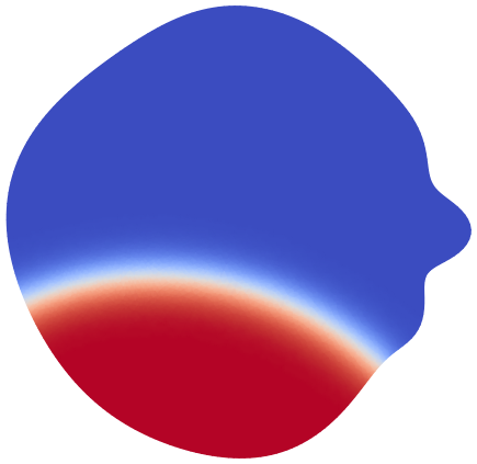
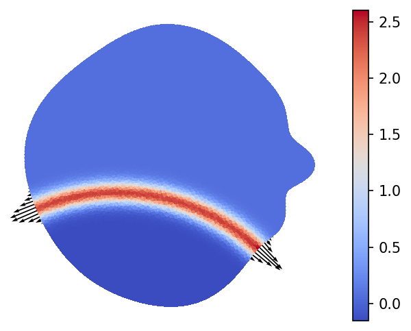
The case of partitions. Consider which minimizes in Theorem 2.8. As in the previous paragraphs, we suppose that is unique and varies smoothly with respect to perturbations in . Differentiating with respect to the domain using the formula (20) we get
| (25) |
Since minimizes under the constraints and there exist Lagrange multipliers , and such that
| (26) |
Since the sum constraint implies that one of the area constraints is redundant we may note that the Lagrange multipliers are not uniquely defined. Adding a constant to and subtracting the same constant from each gives another set of valid multipliers. Therefore, it is not restrictive to assume that the multiplier verifies .
On the other hand, differentiating the constraint gives . Moreover, differentiating the constraints we obtain
Therefore we obtain
| (27) |
The Lagrange multipliers can be found by using in (26), which gives .
As discussed above, in the case is not unique, perturbing the boundary of with normal velocity given by will eventually increase the value of and will reduce the multiplicity of the family of optimal partitions . In Figure 8 the numerical approximation of is shown together with the value of . Perturbing in the normal direction as shown will increase the length of the minimal partition, provided the solution is unique.

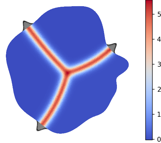
An example of non differentiability - multiplicity greater than one. It is not difficult to imagine domains for which there are multiple minimizers for , given . It is enough to consider small enough and a symmetric domain like in Figure 9. Moreover, there exists a value of for which the Lagrange multiplier vanishes: . It is enough to remember that is proportional to the curvature of the minimal interface as . Let us show that in such a case the functional does not admit a shape derivative. Indeed, suppose that is symmetric like in Figure 9. Denote the two solutions and two vector fields such that (also illustrated in Figure 9).


Suppose that is differentiable at . Then for it is clear that , i.e. the minimal value of does not change when modifying with only one of the vector fields . This would imply that and by linearity . However, this last equality is clearly false, since if we modify with the combined vector field we clearly have
In order to deduce the above equality it is enough to work with one half of the domain . We use the fact that this half can be extended to a non-symmetric domain for which is a unique minimizer and apply the formula for the shape derivative found previously.
Therefore, we arrive at a contradiction, showing that when multiple minimizers of exist, the functional is not shape differentiable. The same kind of argument can be applied for in the case where optimal partitions are not unique.
3.5 Radial parametrization and optimization algorithm
The results of [18] and existence results obtained in Section 2.1 are restricted to convex domains . We therefore choose to search for domains maximizing and in the larger class of star-shaped domains which includes the class of convex sets. These domains can be parametrized using an associated radial function in dimensions two and three. Furthermore, a spectral decomposition of the radial function with a Finite number of Fourier coefficients is used in order to work with a finite, but sufficiently large number of parameters in the computations.
Planar domains. In dimension two, the radial function is discretized using Fourier coefficients
Consider a shape functional whose shape derivative is expressed by . Using the discretization above, given that defines via the radial function , a finite dimensional function is obtained . It is classical to compute the gradient of using the shape derivative, by choosing the appropriate boundary perturbation for each Fourier coefficient. Using the notation we have . Therefore, denoting , we obtain
| (28) |
Domains in . In dimension three we choose to parametrize the unit sphere using . Next, we are interested in parametrizing radial functions which are constant for . This is needed in order to be able to create 3D meshes in FreeFEM [25] by deforming two dimensional meshes. One way of attaining this objective is to use two dimensional Fourier parametrizations which contain only sines for the coordinate, together with an affine function in in order to allow different values at the extremities :
As in dimension two, it is straightforward to infer the gradient of the discretized functional with respect to each one of the parameters. A simple computation yields :
| (29) |
Optimization algorithm. Given the discretization and the gradients expressed above it is straightforward to implement a gradient descent algorithm. The delicate issue is the fact that at each iteration, the objective function and its gradient are computed as a result of a minimization algorithm. If a local minimal perimeter set/partition is found instead of the global one, this might give a wrong ascent direction. Therefore, we choose to work with a gradient flow type algorithm, which consists in advancing at each iteration in the direction given by the gradient of the functional with a prescribed step, regardless of the fact that the objective function increases or decreases. In this way, even the optimization algorithms solved at one of the iterations yields a local minimum, the global optimization algorithm may still correct itself at subsequent iterations. The area constraint is imposed by a projection algorithm: the next iterate is rescaled to have the desired area via a homothety. The precise description is given in Algorithm 3.
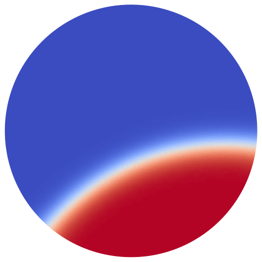
An example of a result obtained with this algorithm for the maximization of is shown in Figure 10 together with the graph of the objective function. It can be seen that the objective function increases and stabilizes as the size of the step decreases. Oscillations in the curve describing the cost have two main causes: first, the optimization algorithm at the current iteration might yield a local minimum instead of the global one and secondly, the size of the step may be too big. An example for the case of partitions is shown in Figure 11. Multiple instances of the gradient flow maximization algorithm are represented in Figure 12 for and in Figure 13 for .


 |
 |
 |
 |
 |
 |
| Iter : | Iter : | Iter : | Iter : | Iter : | Iter : |
 |
 |
 |
 |
 |
 |
| Iter : | Iter : | Iter : | Iter : | Iter : | Iter : |
Numerical aspects. When minimizing and it is classical to consider meshes with elements that have size smaller than . This is due to the fact that the phase transition from to typically takes place in a region of width proportional to and the mesh needs to be fine enough to capture this. In dimension two we consider giving rise to meshes having around nodes.
In dimension three using gives meshes of about nodes. When dealing with more cells in dimension three we start with and we interpolate and re-optimize the result on a finer mesh corresponding to . This gives meshes with around nodes. For postprocessing and plotting purposes, the final mesh is further refined using MMG3D [15] such that more tetrahedra are present where phases change quickly. The final partition is interpolated and re-optimized (with ) on this fine mesh (with around nodes) before plotting.
Code. The finite element software used for the optimization algorithm described in Section 3.1 is FreeFEM [25], which provides an interface to the LBFGS optimizer from Nlopt [28].
The partition initialization via Voronoi diagrams is coded in Python, where optimization algorithms from Scipy.optimize and Nlopt are used for unconstrained and, respectively, constrained optimizations. Codes and examples are provided in the following Github repository: https://github.com/bbogo/LongestShortestPartitions/tree/main/GradientVoronoi.
The visualization is done with Python using Matplotlib in dimension two and Mayavi [39] in dimension three. The graphical representation of partitions is done by extracting surface meshes of an iso-level for each cell in the optimal partition using FreeFEM [25] and MMG3D [15]. These surface meshes are then plotted with Mayavi [39].
Some codes used for obtaining the results illustrated in the paper can be found in the Github repository: https://github.com/bbogo/LongestShortestPartitions/tree/main/FreeFEMcodes.
4 Results
In this section we use the algorithm described previously in order to study problems (3) and (6). Results from [18] show that problem (3) is solved by the disk in dimension two for . We perform simulations for various values of (note that considering or for the constraint gives the same result) and the numerical result is always the disk in dimension two. In dimension three the same phenomenon occurs: for various values of the volume fraction the shape which maximized the relative minimal perimeter of a subset with volume is the ball. Some examples are shown in Figure 14.


Surprisingly, the case of partitions shows similar results. When considering equal area constraints the set with fixed area maximizing the length of the minimal partition is still the disk (see Figure 15 for some examples). In dimension three for we obtain similar results: the ball maximizes the total surface area of the smallest total perimeter partition. These results are illustrated in Figures 17 and 18.


Note that simulations made in the case of one phase already show that when partitioning the domain into two regions with two non-equal areas, the maximizer of the minimal length partition is still the disk. This suggests that even in the case where the cells do not have the same prescribed area, the set which maximizes the minimal perimeter of a partition is still the disk in 2D (the ball in 3D). Indeed, when considering more cells with different areas, the numerical result is the same: the disk seems to be the maximizer (see Figure 16 for some examples). As already underlined in [24], the study of partitions in cells with prescribed but different areas is more complex, since in this case there are even more local minima.
The numerical simulations give rise to the following conjecture, which generalizes the results of [18].
Conjecture 4.1.
1. Given , the set maximizing under the constraint (i.e. solving (3)) is the ball.
2. Given and with , the set maximizing under the constraint (i.e. solving (6)) is the ball.
Remark 4.2.
The same type of results seem to hold when maximizing the minimal geodesic perimeter for closed surfaces in in which are boundaries of convex sets with a constraint on the . The techniques used in this case are those presented in [6] and the theoretical and numerical framework is similar to what was done in dimension three. In this case the sphere seems to be the maximizing set, which is in accord with the conjecture stated above.
5 Remarks on optimality conditions
As discussed in Section 3.4, existence of shape derivatives for and depends on the uniqueness of the minimizers for these functionals. Therefore, it is not straightforward to obtain classical optimality conditions. It is possible, however, to obtain some qualitative information about sets maximizing the minimal values of and under volume constraint. Recall that the optimizer of shape differentiable functional under volume constraint will verify an optimality condition of the form
| (30) |
where is a Lagrange multiplier associated to the volume constraint. Recall that the shape derivative of the volume functional is .
Non-uniqueness of the minimal relative perimeter set/partition at the optimum. Results in Section 3.4 indicate that the shape derivatives of and exist when they correspond to unique minimizers of the Modica-Mortola type functionals. In this case, the corresponding shape derivatives are boundary integrals of non-constant functions multiplied by the normal perturbation . Therefore, it is straightforward to see that a relation of the type (30) cannot hold. This allows us to conclude that of is a minimizer of the optimal minimal relative perimeter set is not unique. The same happens in the case of partitions: if minimizes and the minimal length partition of with constraints is not unique.
Suppose now that is a domain with fixed volume such that is unique. Then for small enough the minimizer of will also be unique. Thus admits a shape derivative. Also the corresponding optimal density is not constant on the boundary, and therefore the optimality relation (30) cannot hold. This shows that such a domain is not a solution of problem (3). The same argument can be applied for problem (6).
6 Conclusions
The theoretical considerations and numerical simulations presented in this paper suggest that the results of [5], [44], [18] are valid in more general settings: in dimensions two and three, under volume and convexity constraints the ball is the set who maximizes
- •
the minimal relative perimeter of a subset with volume constraint for all .
- •
the minimal relative perimeter of a partition of into sets with volume constraints given with . The result seems to hold even in the case where the sets do not have the same volume constraints.
The numerical maximization algorithm consists in solving at each iteration an optimization problem which approximates the least perimeter set or partition under the given constraint. Then a perturbation of the set which does not decrease the minimal perimeter is found and the set is modified. In all cases, the numerical result was close to the disk/ball.
The initialization phase for the computation of the optimal partitions is made using Voronoi diagrams with prescribed capacity. We provide a new way of generating such Voronoi diagrams using the gradients of the areas with respect to the Voronoi points. The gradient of the perimeter of the Voronoi cells is also computed.
Acknowledgments
The authors were partially supported by the project ANR-18-CE40-0013 SHAPO financed by the French Agence Nationale de la Recherche (ANR). The authors thank Frank Morgan for indicating more references to previous works related to the convex isoperimetric problem. The authors thank the reviewers for the careful reading of the manuscript and for their remarks which helped improve the quality of the article.
References
- [1] G. Alberti. Variational models for phase transitions, an approach via -convergence. In Calculus of variations and partial differential equations (Pisa, 1996), pages 95–114. Springer, Berlin, 2000.
- [2] L. Ambrosio, N. Fusco, and D. Pallara. Functions of bounded variation and free discontinuity problems. Oxford Mathematical Monographs. The Clarendon Press, Oxford University Press, New York, 2000.
- [3] M. Balzer. Capacity-constrained voronoi diagrams in continuous spaces. In 2009 Sixth International Symposium on Voronoi Diagrams, pages 79–88, 2009.
- [4] M. Balzer, T. Schlömer, and O. Deussen. Capacity-constrained point distributions: A variant of lloyd’s method. In ACM SIGGRAPH 2009 Papers, SIGGRAPH ’09, New York, NY, USA, 2009. Association for Computing Machinery.
- [5] J. Berry, E. Bongiovanni, W. Boyer, B. Brown, P. Gallagher, D. Hu, A. Loving, Z. Martin, M. Miller, B. Perpetua, and S. Tammen. The convex body isoperimetric conjecture in the plane. Rose-Hulman Undergraduate Mathematics Journal, 18(2), 2017. https://scholar.rose-hulman.edu/rhumj/vol18/iss2/2.
- [6] B. Bogosel and E. Oudet. Partitions of minimal length on manifolds. Exp. Math., 26(4):496–508, 2017.
- [7] J. F. Bonnans and A. Shapiro. Perturbation analysis of optimization problems. Springer Series in Operations Research. Springer-Verlag, New York, 2000.
- [8] A. Braides. Approximation of Free-Discontinuity Problems. Springer, 1998.
- [9] E. Bretin, R. Denis, J.-O. Lachaud, and E. Oudet. Phase-field modelling and computing for a large number of phases. ESAIM Math. Model. Numer. Anal., 53(3):805–832, 2019.
- [10] V. Burenkov. Extension theorems for Sobolev spaces. In The Maz’ya anniversary collection, Vol. 1 (Rostock, 1998), volume 109 of Oper. Theory Adv. Appl., pages 187–200. Birkhäuser, Basel, 1999.
- [11] G. Buttazzo. Gamma-convergence and its Applications to Some Problems in the Calculus of Variations. School on Homogenization ICTP, Trieste, September 6-17, 1993.
- [12] A. Chicco-Ruiz, P. Morin, and M. S. Pauletti. The shape derivative of the Gauss curvature. Rev. Un. Mat. Argentina, 59(2):311–337, 2018.
- [13] A. Cianchi. On relative isoperimetric inequalities in the plane. Boll. Un. Mat. Ital. B (7), 3(2):289–325, 1989.
- [14] S. J. Cox and E. Flikkema. The minimal perimeter for confined deformable bubbles of equal area. Electron. J. Combin., 17(1):Research Paper 45, 23, 2010.
- [15] C. Dapogny, C. Dobrzynski, and P. Frey. Three-dimensional adaptive domain remeshing, implicit domain meshing, and applications to free and moving boundary problems. J. Comput. Phys., 262:358–378, 2014.
- [16] M. C. Delfour and J.-P. Zolésio. Shapes and geometries, volume 22 of Advances in Design and Control. Society for Industrial and Applied Mathematics (SIAM), Philadelphia, PA, second edition, 2011. Metrics, analysis, differential calculus, and optimization.
- [17] Q. Du, V. Faber, and M. Gunzburger. Centroidal voronoi tessellations: Applications and algorithms. SIAM Review, 41(4):637–676, Jan. 1999.
- [18] L. Esposito, V. Ferone, B. Kawohl, C. Nitsch, and C. Trombetti. The longest shortest fence and sharp Poincaré-Sobolev inequalities. Arch. Ration. Mech. Anal., 206(3):821–851, 2012.
- [19] A. V. Fiacco. Introduction to sensitivity and stability analysis in nonlinear programming, volume 165 of Mathematics in Science and Engineering. Academic Press, Inc., Orlando, FL, 1983.
- [20] W. J. Firey. Lower bounds for volumes of convex bodies. Archiv der Mathematik, 16(1):69–74, Dec. 1965.
- [21] D. Gilbarg and N. S. Trudinger. Elliptic partial differential equations of second order. Classics in Mathematics. Springer-Verlag, Berlin, 2001. Reprint of the 1998 edition.
- [22] P. Grisvard. Elliptic problems in nonsmooth domains, volume 24 of Monographs and Studies in Mathematics. Pitman (Advanced Publishing Program), Boston, MA, 1985.
- [23] M. E. Gurtin and H. Matano. On the structure of equilibrium phase transitions within the gradient theory of fluids. Quart. Appl. Math., 46(2):301–317, 1988.
- [24] F. Headley and S. Cox. Least perimeter partition of the disc into n bubbles of two different areas. The European Physical Journal E, 42(7), July 2019.
- [25] F. Hecht. New development in FreeFem++. J. Numer. Math., 20(3-4):251–265, 2012.
- [26] A. Henrot and M. Pierre. Shape variation and optimization, volume 28 of EMS Tracts in Mathematics. European Mathematical Society (EMS), Zürich, 2018. A geometrical analysis, English version of the French publication [ MR2512810] with additions and updates.
- [27] M. Iri, K. Murota, and T. Ohya. A fast voronoi-diagram algorithm with applications to geographical optimization problems. In System Modelling and Optimization, pages 273–288. Springer-Verlag.
- [28] S. G. Johnson. The nlopt nonlinear-optimization package. http://github.com/stevengj/nlopt.
- [29] B. Kloeckner. Dans quelle forme la plus petite paroi enfermant un volume donné est-elle la plus grande ? - Images des mathématiques : http://images.math.cnrs.fr/Dans-quelle-forme-la-plus-petite-paroi-enfermant-un-volume-donne-est-elle-la.html, 12 2019.
- [30] A. Koldobsky, C. Saroglou, and A. Zvavitch. Estimating volume and surface area of a convex body via its projections or sections. Studia Math., 244(3):245–264, 2019.
- [31] S. Luckhaus and L. Modica. The Gibbs-Thompson relation within the gradient theory of phase transitions. Arch. Rational Mech. Anal., 107(1):71–83, 1989.
- [32] F. Maggi. Sets of finite perimeter and geometric variational problems, volume 135 of Cambridge Studies in Advanced Mathematics. Cambridge University Press, Cambridge, 2012. An introduction to geometric measure theory.
- [33] L. Modica. The gradient theory of phase transitions and the minimal interface criterion. Arch. Rational Mech. Anal., 98(2):123–142, 1987.
- [34] L. Modica and S. Mortola. Un esempio di -convergenza. Boll. Un. Mat. Ital. B (5), 14(1):285–299, 1977.
- [35] F. Morgan. Soap bubbles in and in surfaces. Pacific J. Math., 165(2):347–361, 1994.
- [36] F. Morgan. Convex body isoperimetric conjecture. https://sites.williams.edu/Morgan/2010/07/03/convex-body-isoperimetric-conjecture/, 2010.
- [37] É. Oudet. Approximation of partitions of least perimeter by -convergence: around Kelvin’s conjecture. Exp. Math., 20(3):260–270, 2011.
- [38] G. Polya. Aufgabe 283. Elem. d. Math., 13:40–41, 1958.
- [39] P. Ramachandran and G. Varoquaux. Mayavi: 3d visualization of scientific data. Computing in Science Engineering, 13(2):40–51, 2011.
- [40] M. Ritoré and E. Vernadakis. Isoperimetric inequalities in Euclidean convex bodies. Trans. Amer. Math. Soc., 367(7):4983–5014, 2015.
- [41] J. Sokoł owski and J.-P. Zolésio. Introduction to shape optimization, volume 16 of Springer Series in Computational Mathematics. Springer-Verlag, Berlin, 1992. Shape sensitivity analysis.
- [42] P. Sternberg and K. Zumbrun. Connectivity of phase boundaries in strictly convex domains. Arch. Rational Mech. Anal., 141(4):375–400, 1998.
- [43] K. Svanberg. A class of globally convergent optimization methods based on conservative convex separable approximations. SIAM Journal on Optimization, 12(2):555–573, Jan. 2002.
- [44] B.-H. Wang and Y.-K. Wang. A note on the convex body isoperimetric conjecture in the plane, 2021.
- [45] W. Wichiramala. Efficient cut for a subset of prescribed area. Thai J. Math., 5(3, Special issue):95–100, 2007.
- [46] S.-Q. Xin, B. Lévy, Z. Chen, L. Chu, Y. Yu, C. Tu, and W. Wang. Centroidal power diagrams with capacity constraints: Computation, applications, and extension. ACM Trans. Graph., 35(6), Nov. 2016.