A crystal symmetry-invariant Kobayashi–Warren–Carter grain boundary model and its implementation using a thresholding algorithmJournal: Journal of Computational Materials Science

The Kobayashi–Warren–Carter (KWC) model (Kobayashi et al. 1998; Kobayashi et al. 2000; Warren et al. 2003) is a dual-phase field model to study grain evolution in polycrystalline materials. In this model, an arbitrary polycrystal in two dimensions is described using only two order parameters $\eta$ and $\theta$. This is one of the main advantages of employing the KWC model as opposed to the multiphase field model, which uses as many order parameter as the number of grains. The order parameter $\eta$ ranges from $0$, which signifies disorder, to $1$ that describes crystalline order. On other hand, the order parameter $\theta$ describes the orientation of the grains.³³ 3 In three dimensions, the order parameter $\theta$ is replaced by a rotation tensor.

The KWC model is governed by a free energy functional given by

where

is a single-well potential with minimum at $\eta=1$, and

is an increasing function.⁴⁴ 4 The choice of the logarithmic function for $g$ is supported by the work of Alicandro et al. 1999, which shows that the KWC functional converges (in the sense of $\Gamma$-convergence) to a surface energy function when $g(1)=\infty$ (See Theorem 4.1 in Alicandro et al. 1999). The functional in (2.1) is defined for all functions $\eta$ and $\theta$ in the Hilbert space $H^{1}(\Omega)$.⁵⁵ 5 $H^{1}(\Omega)$ denotes the set of all functions on $\Omega$ whose first derivatives are square integrable. The constant $\epsilon>0$ is a dimensionless scaling parameter that determines the thickness of the grain boundary region (Lobkovsky and Warren 2001). The evolution equations for the order parameters, assuming a gradient descent (with respect to the $L^{2}$-norm) of $\mathcal{W}$, are obtained as

where $b_{\eta}$ and $b_{\theta}$ are the inverse mobilities corresponding to respective order parameters.⁶⁶ 6 The KWC model was originally developed to simultaneously model grain rotation and grain boundary motion. The model can be specialized to demonstrate only grain boundary motion by enforcing zero mobility for $\theta$ in the grain interior. This can be achieved by a constant $b^{\phi}$, and a $\phi$-dependent $b^{\theta}$ (Dorr et al. 2010).

A one-dimensional steady state solution of (2.4) under Dirichlet boundary conditions is plotted in Fig. 2(a). The value of $\eta<1$ in a neighborhood of the grain boundary suggests a loss of crystalline order, and the orientation $\theta$ is constant in the interior of the grains, and has a non-zero gradient in a finite thickness around the grain boundary. In the limit $\epsilon\to 0$, Lobkovsky and Warren 2001 have shown that the evolution equations in (2.4) result in the shrinking of the grain boundary thickness converging to the Mullins model.

Below, we briefly summarize the role of each term appearing in the KWC functional. We refer the reader to Warren et al. 2003 for a more detailed description, and Admal et al. 2019 for a generalization of the KWC model to three dimensions. The function $f$ drives $\eta(\bm{x})$ towards $1$, while the coupled term $g(\eta)|\nabla\theta|$ tends to decrease $\eta$ in a neighborhood of the grain boundary. In addition, the coupled term tends to localize the jump in $\theta$, while $|\nabla\theta|^{2}$ has a tendency to diffuse it, resulting in a regularized step function for $\theta$. It is interesting to note that in the absence of the $|\nabla\theta^{2}|$ term, the steady state solution for $\theta$ is a pure step function, resulting in a model with a blend of sharp- and diffuse-interface characteristics, i.e. while $\theta$ is sharp, $\eta$ is diffused. Moreover, grain boundaries cease to evolve in the absence of $|\nabla\theta|^{2}$ term (Lobkovsky and Warren 2001). In other words, $|\nabla\theta|^{2}$ in the KWC model has a dual role of not only regularizing $\theta$ but also rendering non-zero mobility to the grain boundaries.

The grain boundary energy $\gamma$, as a function of misorientation angle, predicted by the KWC model is of the Read–Shockley-type, as shown in Fig. 2(b). This is in contrast to the experimentally observed grain boundary energies shown in Fig. 1. Despite the elegance of the KWC model in describing polycrystals with only two order parameters, its restriction to Read–Shockley type grain boundary energies is a major limitation compared to the flexibility of incorporating arbitrary grain boundary energies into the multiphase field model. The above-stated limitation is one of the main motivation for us to seek a new formulation of the KWC model to incorporate arbitrary misorientation-dependent grain boundary energies that respect the bicrystallography of grain boundaries.

In this section, we formulate a new KWC model that can incorporate arbitrary misorientation-dependent grain boundary energies.

We begin with the KWC functional without the $|\nabla\theta|^{2}$ term. From Section 2.1, recall that in the absence of the $|\nabla\theta|^{2}$ term, the steady state solution for $\theta$ is a step function with the discontinuity occurring at the grain boundary. In one-dimension, since a discontinuous $\theta$ is not in $H^{1}(\Omega)$, the minimizer of $\mathcal{W}$, with $|\nabla\theta|^{2}$ absent, is not attained. This observation motivates us to redefine the domain of the modified KWC functional such that $\theta$ belongs to the space of piecewise constant functions, as opposed to $H^{1}(\Omega)$, and this enables us to simplify the functional as

where $\bar{\eta}:\mathcal{S}\to\mathbb{R}$ is the restriction of $\eta$ to the jump set $\mathcal{S}$ of $\theta$, which represents the union of all grain boundaries. The steady state solution, given in (A.8), corresponding to a one-dimensional bicrystal governed by (2.5), and the resulting grain boundary energy as a function of the misorientation,

are derived in A. From (2.6), it is clear that the grain boundary energy is of a Read–Shockley-type, which does not respect the crystal symmetry.

The above observation leads us to the following generalization of the KWC functional

which is defined for all $\eta\in H^{1}(\Omega)$, and piecewise constant functions $\theta$; and $\mathcal{J}$ is an even function of the jump in orientation. Under this new formulation, the grain boundary energy function modifies as

where $\bar{\eta}$ is the value of the stead-state solution on the grain boundary, given implicitly in terms of $\mathcal{J}(\llbracket\theta\rrbracket)$ as⁷⁷ 7 The analog of (2.9) in the original KWC model is (A.7), whose derivation is shown in A.

Inspired from the terminology in dislocations, we refer to $\mathcal{J}(\llbracket\theta\rrbracket)$ as the core energy.

From (2.8), it is clear that by appropriately constructing the core energy $\mathcal{J}$, we can arrive at a $\gamma^{\rm G}$ that faithfully represents the grain boundary energy and symmetry of the bicrystal. In other words, the crystal symmetry of the new KWC model is inherited from the core energy. For illustration, we consider the energy $\gamma^{\rm cov}$ of a $[110]$ symmetric tilt grain boundary in face-centered cubic (fcc) copper, shown as red data points in Fig. 3. $\gamma^{\rm cov}$ is computed using the covariance model developed by Runnels et al. 2016a; Runnels et al. 2016b, wherein it is defined as the covariance of the two lattices adjoining the grain boundary. For completeness, in B, we describe the covariance model of grain boundary energy, the procedure to compute it, and list the parameters used to arrive at the data plotted in Fig. 3. We solve for $\mathcal{J}$ in (2.8) using the Newton’s method such that the resulting $\gamma^{\rm G}=\gamma^{\rm cov}$ at each data point. In other words, the grain boundary energy of the resulting KWC model is identical to $\gamma^{\rm cov}$ by construction. Fig. 3 shows a plot of the solution $\mathcal{J}$ in green, and highlights the common positions of the local minimizers of $\mathcal{J}$ and $\gamma^{\rm cov}$. Typically, the number of Newton iterations for convergence error (absolute value of the difference between $\gamma^{\rm G}$ and $\gamma^{\rm cov}$) of $10^{-6}\rm[J/m^{2}]$ is less than 20. While the modification of the KWC functional from (2.5) to (2.7) allows us to model arbitrary misorientation-dependent grain boundary energies, the absence of $|\nabla\theta|^{2}$ term in (2.7) renders the grain boundaries immobile as mentioned in Section 2.1.⁸⁸ 8 The evolution of $\theta$ by the gradient descent of $\mathcal{W}^{\rm G}$ results in pure rotation while the position of the grain boundaries remains fixed. In what follows, we address this shortcoming by devising a thresholding method to move grain boundaries by evolving the piecewise-constant $\theta$.

A thresholding method is a sequence of simple rules, executed every time step to reinitialize the order parameter, such that its evolution describes the motion of a grain boundary.

The original idea of using a thresholding method to evolve grain boundaries goes back to the work (Merriman et al. 1992) of Merriman, Bence and Osher (MBO) wherein, similar to the multiphase field model, grains in a polycrystal are described using as many order parameters, with the caveat that the order parameters are piecewise-constant implying a sharp interface. An order parameter in the MBO method is evolved based on a two-step thresholding scheme — a convolution of the order parameter with a Gaussian kernel followed by a trivial thresholding — resulting in motion by curvature.

The MBO method has recently been generalized by Esedoḡlu and Otto 2015 to a variational model, referred to as the Gaussian kernel method. In the MBO and the Gaussian kernel methods, there are as many characteristic functions as the number of distinct grains. While the end goal of the KWC model is also to describe motion by curvature, it is markedly different from the Gaussian kernel method as it uses only two order parameters to represent a polycrystal. Therefore, it does not require additional techniques to address the memory intensive nature of a naive implementation of the MBO/Gaussian kernel methods. More importantly, the KWC model lends itself to further generalizations which include the modeling of grain rotation. Therefore, the goal here is to seek a thresholding algorithm to implement the KWC model.

In this section, we design a thresholding rule for $\theta$ that results in motion by curvature. We first recall that $\theta$ is a piecewise-constant field with a finite range of orientations. This implies, that a thresholding rule for $\theta$ reassigns $\theta(\bm{x})$, for each point $\bm{x}\in\Omega$, to one of the possible orientations. Our thresholding rule originates from the observation that the asymmetry of $\eta$ in the neighborhood of a grain boundary characterizes its curvature. Below, we explicitly identify this asymmetry before describing our thresholding rule.

First, we note that the steady-state solution for $\eta$, derived in (A.8) for a flat interface (zero curvature), is symmetric about the grain boundary. Next, we derive an approximate form for $\eta$ in the presence of a non-zero curvature, and show the dependence of asymmetry on the curvature. Let $\Gamma$ denote a grain boundary with a non-zero curvature that separates two grains with orientations $\theta_{\rm L}$ and $\theta_{\rm R}$. We postulate that for a $\Gamma$ with a small curvature such that $\epsilon\kappa\ll 1$, and for a $\bm{x}_{0}\in\Gamma$ away from a triple junction, the solution $\eta^{*}$ to (2.4a) is approximated in a small neighborhood of $\bm{x}_{0}$ as

where $l(\bm{x})$ is the signed distance function from $\Gamma$ to $\bm{x}$, as shown in Fig. 4. In other words, we assume that $\eta$ only depends on the radial coordinate. Away from the grain boundary, the solution to the minimization problem in (3.1) satisfies the equation

The above equation can be simplified by using a local coordinate system $\bm{x}=(\tilde{l},s)$, where $\tilde{l}=l(\bm{x})/\epsilon$ is the scaled radial coordinate, and $s$ is the distance measured along $\Gamma$ between $\bm{x}_{0}$ and the perpendicular projection of $\bm{x}$ on $\Gamma$. In this coordinate system, we note that $\triangle\eta(\bm{x})=u^{\prime\prime}/\epsilon^{2}+\kappa u^{\prime}/\epsilon$, where $\kappa(\tilde{l})$ is the curvature of the coordinate line $\{\bm{x}\in B_{r}(\bm{x}_{0}):l(\bm{x})=\tilde{l}\epsilon\}$. Therefore, (3.3a) simplifies as

Assuming $\kappa(\tilde{l})=\kappa(0)$, we obtain the following closed form solution to (3.4):

where the constants $C_{1}$ and $C_{2}$ are determined using the boundary conditions $u(\pm\infty)=1$.⁹⁹ 9 The boundary conditions are interpreted in the limit $\epsilon\to 0$, which results in the boundary conditions $l/\epsilon=\pm\infty$ for the scaled radial coordinate. Subsequently, the solution can be further approximated¹⁰¹⁰ 10 Here, we use the approximation $\sqrt{4+\epsilon^{2}\kappa^{2}}\approx 2+\mathcal{O}(\epsilon^{2}\kappa^{2})$. under the assumption that both $\epsilon$ and $\epsilon\kappa$ are small, resulting in

The asymmetry of $u$ is apparent from (3.6) by noting that in the presence of a positive curvature, the rate at which $u\to 1$ as $\tilde{l}\to+\infty$ is greater than when $\tilde{l}\to-\infty$.

The asymmetry of $u$ forms the foundation of our thresholding scheme, which is designed to reassign the values of $\theta$ in the neighborhood of the grain boundaries resulting in a motion by curvature. To design a thresholding rule, we identify a unique $l=l_{0}$, such that

The two integrals in (3.7) are depicted as equal areas under the yellow and green regions in Fig. 5, which clearly shows that in the presence of a non-zero curvature, the asymmetry of $u$ results in $l_{0}\neq 0$. A straightforward but tedious calculation (see D for details) shows that

By reinitializing the orientations of all $\bm{x}$ with $l(\bm{x})<l_{0}$ to $\theta_{\rm L}$, and to $\theta_{\rm R}$ when $l(\bm{x})>l_{0}$, we have a thresholding rule that moves the grain boundary by $\epsilon^{2}\kappa$ in one time step $dt=\mathsf{t}\epsilon^{2}/4$, where $\mathsf{t}=1$ is a unit conversion factor. Alternating between the $\eta$-update using the primal-dual method, and the $\theta$-update using the thresholding rule, results in a grain boundary motion by curvature with mobility equal to the inverse of the grain boundary energy.¹¹¹¹ 11 In this case, the reduced mobility (Salvador and Esedoḡlu 2019; Martine La Boissonière et al. 2019), which is defined as the product of grain boundary energy and mobility, is equal to $1$ for all grain boundaries. Although this is a severe restriction on the mobility, we postulate that this can be overcome by modifying the thresholding rule (3.7), and this will be addressed in a future work. The efficiency of the thresholding rule described above rests on the computation of $l_{0}$ in (3.7). In the next section, we use the fast marching method to not only compute $l_{0}$ in an $\mathcal{O}(N\log N)$ algorithm, but also generalize the above strategy to an arbitrary polycrystal.

The fast marching method (FMM), developed by Tsitsiklis 1995, is an algorithm to evolve a surface with a spatially varying normal velocity. A general description of FMM with a stand-alone example is given in E. Here, we focus on using the fast marching method to implement the thresholding algorithm described in Section 3.1 by solving for $l_{0}$ in (3.7).

We begin with a description of our implementation of the thresholding scheme for a bicrystal consisting of a circular grain, followed by its generalization to a polycrystal. We first recall that the boundary conditions $u(\pm\infty)=1$ used to arrive at (3.6)–(3.7) apply only in the limit $\epsilon\to 0$ as noted in footnote 9. In practice, we choose a finite limit $l_{\rm b}>0$, and modify (3.7) as

In D, we show that the error in $l_{0}$ due to the introduction of $l_{\rm b}$ exponentially decreases as $\epsilon\to 0$. In order to use FMM to compute $l_{0}$, we interpret the integrand $(1-u(l/\epsilon))^{2}$ in (3.9) as an inverse of the normal velocity of a surface $\mathcal{S}_{l}:=\{\bm{x}:l(\bm{x})=l\}$ traveling towards the grain boundary. Under this interpretation, the integrals in (3.9) are a measure of the time it takes for two initial surfaces $\mathcal{S}_{-l_{\rm{b}}}$ and $\mathcal{S}_{l_{\rm b}}$ on either side of the grain boundary, to meet at $l=l_{0}$. We use the fast marching method to evolve the surfaces $\mathcal{S}_{-l_{\rm{b}}}$ and $\mathcal{S}_{l_{\rm b}}$, and implement the thresholding rule described in Section 3.1 by reassigning the orientation of any point $\bm{x}$ in the region $\{\bm{x}\in\Omega:|l(\bm{x})|<l_{\rm b}\}$ to $\theta_{\rm L}$ if it first encounters the evolving surface $\mathcal{S}_{-l_{\rm b}}$, and to $\theta_{\rm R}$ otherwise.

In practice, however, we do not have access to the signed distance function $l(\bm{x})$ to identify the surfaces $\mathcal{S}_{-l_{\rm b}}$ and $\mathcal{S}_{l_{\rm b}}$. Instead, we first identify the grain interiors $I_{p}$ defined as

where $\xi>0$ is some fixed small value. Fig. 6(a) shows the grain interiors $I_{1}$ and $I_{2}$ in a bicrystal, and Fig. 6(b) is a closeup of a rectangular region, marked in yellow, around the grain boundary. The original grain boundary is marked as a black dashed line in Fig. 6(b). By construction, the two surfaces $\partial I_{1}$ and $\partial I_{2}$ are equidistant, up to $\mathcal{O}(\epsilon)$, from the grain boundary, and serve as substitutes for $\mathcal{S}_{-l_{\rm b}}$ and $\mathcal{S}_{l_{\rm b}}$. The grain interiors are grown in the outward direction with a velocity $(1-u(l/\epsilon))^{-2}$ using the fast marching method, and the surface where they meet is the new grain boundary, shown as a green dashed line in Fig. 6(b).

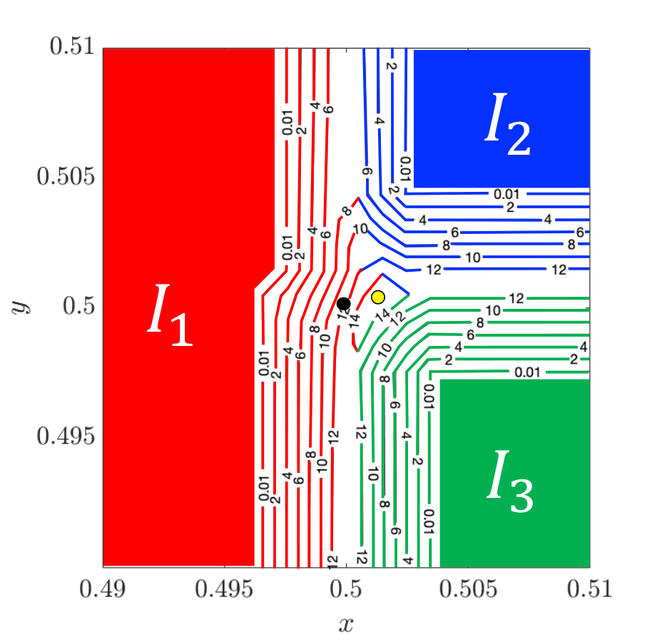
We will now generalize the above implementation to an arbitrary polycrystal consisting of $\mathcal{N}$ grains, described using a piecewise constant $\theta$ with values in $\{\theta_{1},\dots,\theta_{\mathcal{N}}\}$. Using (3.10), we identify the $\mathcal{N}$ grain interiors, and define $I$ as their union. Next, we grow the grain interiors in their outward unit normal directions until every point (in the almost everywhere sense) in the domain is in precisely one grain. We implement this by first collecting all the boundaries of the interior regions in $\partial I=\partial I_{1}\cup\dots\cup\partial I_{n}$, and simultaneously evolving them in the outward normal direction with a speed of $1/(1-\eta^{*}(x))^{2}$ using the fast marching method.¹²¹² 12 Note that the fast marching method is used to evolve all grain interiors in unison as opposed to evolving them individually. As the grain interiors grow, a point $\bm{x}\in\Omega-I$ is reinitialized to an orientation $\theta_{q}$ if it encounters $\partial I_{q}\subset\partial I$. At the end of the fast marching method, all points in $\Omega-I$ have been reinitialized resulting in an updated polycrystal at the end of a time step. Fig. 7 shows the implementation of the thresholding rule in a tricrystal. Dirichlet boundary conditions on $\theta$ are imposed by including all $\bm{x}\in\partial\Omega$ in the grain interiors. On the other hand, periodic boundary conditions are achieved by periodically reinitializing $\theta$ for $\bm{x}\in\partial\Omega$ during the fast marching step.

The primal-dual and the fast marching methods are implemented on a regular grid of resolution, say $\delta x$. From (3.8), we know that the resolution of the grid should be large enough to resolve a grain boundary movement of $\epsilon^{2}\kappa$ in each time step, i.e.

which is a common requirement of other thresholding methods (Esedoḡlu and Otto 2015; Merriman et al. 1992). If this condition is not satisfied, grain boundaries would stagnate. Since grain boundary evolution results in an overall decrease in curvature, (3.11) may cease to hold as the simulation progresses. Therefore, we adaptively increase $\epsilon$ when a grain boundary stagnates, and as a consequence, we obtain a time adaptive algorithm since $dt\propto\epsilon^{2}$. On the other hand, an extremely small $\epsilon$ will increase the computational cost of the thresholding method.

Finally, we explore the effect of $\xi$, introduced in (3.10), on the extent to which (3.8) is satisfied. Recall that $\xi$ was introduced in (3.10) to identify grain interiors. In the case of a circular grain (see Fig. 6(a)), (3.8) implies the rate of change of radius is given by

To test if the above equation is satisfied, we executed the thresholding algorithm using the $\eta$-solution from the primal dual algorithm with $\epsilon=0.01$, and measured $\dot{R}(t)$. Relative % errors in shrinking-rate $\dot{R}$ at different values of $\xi$ are summarized in Tab. 1. It is confirmed that for a sufficiently small grid, $\xi=0.05$ is small enough to achieve an error less than 1%.

Algorithm 1 summarizes our approach. The core energy data $\mathcal{J}$ (e.g., Fig. 3) is computed separately using the procedure described in Section 2.2, and used as an input to our method. The algorithm alternates between the primal-dual and the fast marching methods resulting in motion by curvature. A C++ template library that implements Algorithm 1 is available at https://github.com/admal-research-group/GBthresholding.

Finally, we remark on the computation of $\mathcal{J}(\bm{x})$ on a grid. Since $\llbracket\theta\rrbracket$, calculated at a grid point $ij$ in either $x$- or $y$-directions using centered-difference, is shared between two grid points, a factor of $1/2$ appears in the following expression used to compute the total jump:

A triple junction is a line where three grains meet, and it is represented as a point in two dimensions. The equilibrium of a triple junction is guaranteed if it satisfies the Herring relation (Herring 1951) given by

where $\Theta_{i}$ is the dihedral angle of grain $i$, and $\gamma^{ij}$ is the energy density of the grain boundary shared by grains $i$ and $j$. While the Herring relation is derived in the sharp-interface framework, it is also seen to hold for a triple junction governed by the original KWC model through (2.4). This is not surprising since the KWC model converges to the Mullins model in the sharp-interface limit and the evolution in (2.4) has a variational structure in the form of a gradient descent of the functional in (2.1). On the other hand, it is not clear if our approach to evolve the generalized KWC model arises from a variational formulation. Therefore, it is necessary to examine the Herring relation using our thresholding algorithm. We will now demonstrate that the Herring relation indeed holds provided the parameter $\epsilon$ is chosen appropriately.

We study the evolution of a triple junction in a tricrystal with orientations $\theta_{1}=0$, $\theta_{2}=\pi/6$, and $\theta_{3}=\pi/3$ in $\Omega=[0,1]\times[0,1]$. Using the Read–Shockley core energy $\mathcal{J}=\llbracket\theta\rrbracket$, we note from Fig. 8(b) that the energy density of the three grain boundaries are $\gamma^{12}=0.62$, $\gamma^{23}=0.62$, and $\gamma^{13}=0.87$. From the Herring relation in (4.1), it follows that the steady state dihedral angles are $\Theta_{1}=134.56^{\circ}$, $\Theta_{2}=90.89^{\circ}$, and $\Theta_{3}=134.56^{\circ}$. In order to examine the Herring relation, we consider a tricrystal under periodic boundary conditions, with an initial orientation distribution given by

resulting in four triple junctions at $(x_{1},x_{2})=(0.25,0.75),(0.75,0.75),(0.75,0.25)$, and $(0.25,0.25)$. The initial dihedral angles of the triple junctions are $90^{\circ}$, $180^{\circ}$, and $90^{\circ}$. Fig. 9(a) shows a plot of the initial orientation distribution of the tricrystal.

We begin by comparing the evolution of a triple junction predicted by the KWC model implemented using our thresholding scheme with that obtained using the Gaussian kernel method (Esedoḡlu and Otto 2015). The grain boundary energies $(\gamma^{12},\gamma^{23},\gamma^{13})=(0.62,0.62,87)$, pre-computed using the KWC model, are inputs to the Gaussian kernel method, and the respective mobilities are set to the inverse of the grain boundary energies. The parameter $\epsilon$ of the KWC model is taken as $0.01$. Both schemes are simulated on a $1024\times 1024$ grid. As shown in Fig. 9, the evolution dynamics of both schemes are qualitatively similar. As expected, the triple junction adjusts at a faster time scale to satisfy the Herring angle condition compared to the curvature-driven motion of grain boundaries (Esedoḡlu et al. 2010). The motion of triple junctions induces a curvature in the grain boundaries, which drives the shrinking of the embedded grains (blue and yellow), while maintaining constant dihedral angles. The dihedral angles predicted by the Gaussian kernel method are $(93^{\circ},133.5^{\circ},133.5^{\circ})$, while the generalized KWC model with $\epsilon=0.01$ yields $(106^{\circ},127^{\circ},127^{\circ})$.

To further investigate the dependence of the triple junction angles on $\epsilon$, we implement the thresholding algorithm with $\epsilon=0.01$, $0.006$ and $0.003$ on a $3000\times 3000$ grid. As shown in Fig. 10(b) to Fig. 10(d), as $\epsilon$ decreases, the stabilized triple junction angles converge to those predicted by the Herring relation. This test suggests that the Herring relation is satisfied in the limit $\epsilon\to 0$.

In this section, we validate our thresholding scheme by testing the von Neumann–Mullins relation for a polycrystal with uniform grain boundary energies ($\gamma$) and mobilities ($m$). In two dimensions, the von Neumann-Mullins law (von Neumann 1952; Mullins 1956) states

where $A$ is the area of a grain with $n$ sides, and $\gamma$ . In other words, grains with more than six sides grow, while those with less than six sides will shrink.

To test the relation given in (4.3), we select the core energy function as a constant ($\mathcal{J}(\llbracket\theta\rrbracket)=0.5$), and consider an initial polycrystal consisting of $\mathcal{N}=50$ grains. The initial configuration, shown in Fig. 11(a), is generated using a Voronoi tessellation of uniformly distributed random points. We implemented Algorithm 1 with parameters $\epsilon=0.01$, $\mathsf{e}=10^{-6}$, and $\xi=0.05$, on a $1024\times 1024$ grid.

As described in Section 4.1, the evolution of the polycrystal begins with the motion of triple junctions to attain the dihedral angles $(120^{\circ},120^{\circ},120^{\circ})$ predicted by (4.1) for constant $\gamma$. Subsequently, grain boundary motion by curvature follows. A snapshot of an evolving grain microstructure at $t=5\times 10^{-3}$, simulated using our thresholding scheme, is shown in Fig. 11(b). In Fig. 12, we plot the mean rate of change of area of grains — along with standard deviation — measured during the time interval $[2.5\times 10^{-3},5.0\times 10^{-3}]$, as a function of the number of sides. Noting that the plot in red is close to the theoretically predicted black dashed line, we confirm that our thresholding scheme accurately predicts the von Neumann-Mullins law.

In this section, we compare the evolutions of a polycrystal resulting form our thresholding method and a finite element implementation of the KWC model, which we will refer to as FE-KWC. An initial polycrystal consisting of $\mathcal{N}=50$ grains, as shown in Fig. 13(a), is generated using a Voronoi tessellation of uniformly distributed random points. The orientations of the grains are randomly chosen from the interval $[0,\pi/2]$. The core energy is chosen to be of the Read–Shockley-type, i.e. $\mathcal{J}=\llbracket\theta\rrbracket$.

The thresholding algorithm is implemented on a $1024\times 1024$ grid, with parameters $\epsilon=0.01$, $\mathsf{e}=10^{-6}$, and $\xi=0.05$. A snapshot of an evolving grain microstructure at $t=5\times 10^{-3}$, simulated using our thresholding scheme, is shown in Fig. 13(b).

We note that FE-KWC, using continuous Lagrange finite elements, cannot be carried out on our model since the solution for $\theta$ is discontinuous. Therefore, we proceed with a finite element implementation of the regularized KWC model given in (2.4). We use second-order quadrilateral Lagrange finite elements to interpolate the order parameters. Since the regularized model allows grain rotation, we inhibit rotation using the following $\eta$-dependent mobility for $\theta$

as suggested by Dorr et al. 2010. On the other hand, $(b_{\eta})^{-1}=\epsilon$ is chosen to be constant. To address the singularity due to the $|\nabla\theta|$ term in (2.4b), we use the approximation

where $\rho_{0}=2\times 10^{-3}$ is a constant. The manifestation of $\rho_{0}$ on the solution will be discussed below. FE-KWC is performed on the open-source computing platform Fenics Alnaes et al. 2015. We take an implicit time step with $dt=0.012$. In order to compare the numerical efficiency, we ensure that the number of degrees of freedom is the same in the thresholding and the finite element simulations. The grain microstructure at $t=1.71$, simulated using FE-KWC, is shown in Fig. 13(c).

Comparing Figs. 13(b)–13(c), we note that both the methods are consistent in predicting growth (see \footnotesize{1}⃝, \footnotesize{2}⃝) and shrinkage (see \footnotesize{3}⃝, \footnotesize{4}⃝) in various grains. It is observed that grain boundaries become rounded in the finite element simulation, because of the diffusive nature of orientation field. In addition, disparities are more clear for small misorientation grain boundaries, e.g. \footnotesize{5}⃝, which are highly diffused. This is a manifestation of $\rho_{0}$, which results in a non-zero gradient in $\theta$ in the grain interiors. In Fig. 14, we compare two finite element simulations with $\rho_{0}=2\times 10^{-3}$ and $2\times 10^{-4}$, which shows that for a smaller $\rho_{0}$, the grain boundaries retain their characteristic width.¹³¹³ 13 Recall that the characteristic width of a grain boundary in the regularized KWC model is a function of $\epsilon$. Thus, to simulate sharp grain interfaces comparable to the our scheme, a small enough $\rho_{0}$ is required for FE-KWC. However, we note that the decrease in $\rho_{0}$ increases the stiffness of the equations, which significantly affects the computational time as discussed below.

Computational time study clearly highlights the advantage of the our thresholding scheme. Performance tasks are executed on a single 1.6 GHz core with 8 GB RAM, and we measured the wall-clock time to complete one-full time step for the two methods. For our method, this includes solving for $\eta$ using the primal dual algorithm, and executing the fast marching based thresholding algorithm to update $\theta$. In Fig. 15, we plot the dependence of the wall-clock time, as a function of the number of degrees of freedom $N$. The computational complexity of the current scheme is $\mathcal{O}(N\log{N})$, with a dominant contribution from FFT used in the primal dual algorithm to solve (C.7). On the other hand, the asymptotic computational cost of FE-KWC is estimated to be in between $\mathcal{O}(N)$ and $\mathcal{O}(N^{2})$ as shown in Fig. 15. The computational bottleneck of FE-KWC is in solving — using a GMRES iterative solver (Saad and Schultz 1986) — a linear system of equations formed by an $N\times N$-sized sparse matrix. Though the asymptotic costs of the two schemes are similar in terms of $N$, we note that the computational cost of FE-KWC also depends on the choice of the regularization parameter $\rho_{0}$, which increases the stiffness of the equations in the limit $\rho\to 0$. Therefore, as demonstrated in Fig. 15, the current scheme can be orders of magnitude faster than FE-KWC. Both, FE-KWC and the implementation of our method, can be well-parallelized using the current generation of graphics cards, which have the power, programmability and precision to implement FFT and iterative matrix solvers (Li and Saad 2013; Govindaraju et al. 2008) respectively.

In this section, we examine grain growth in a two-dimensional fcc copper polycrystal with $[110]$-type grain boundaries simulated using the generalized KWC model,¹⁴¹⁴ 14 The $[110]$ direction of each grain is is aligned with the $z$-axis (out of the plane). with crystal symmetry-invariant grain boundary energy. We compare the results with the predictions of the original KWC model.

A two-dimensional polycrystal consisting of $\mathcal{N}=50$ grains, with orientations in the range $[0,70.6^{\circ}]$ is generated using a Voronoi tessellation of random points. Fig. 17 shows the initial orientation distribution in the polycrystal. We assume that the grain boundary energy density is independent of inclination. We use the core energy $\mathcal{J}(\llbracket\theta\rrbracket)$ constructed in Section 2.2 (see Fig. 3). In order to compare the generalized model to the original KWC model, we scale the function $g$ of the original KWC model in (2.1) to $g=-0.93\ln(1-\eta)$ such that the mean of the grain boundary energies as functions of misorientation in the range $[0,70.6^{\circ}]$ are identical for the two models. Fig. 16 shows a comparison of the grain boundary energy densities of the two models.

The orientation distributions of the polycrystal at the end of 200 time steps for the generalized and the original KWC models are shown in Figs. 17(b)–17(c) respectively. Comparing the resulting polycrystals with the initial polycrystal in Fig. 17(a), we note that the generalized KWC model predicts a growth for red grains while the original model results in their shrinkage. This can be attributed to the difference in the grain boundary energies of the two models, as shown in Fig. 18. For example, the grain boundary \footnotesize{1}⃝, which has a misorientation of $\approx 70.6^{\circ}$ has a relatively smaller energy in the generalized model due to crystal symmetry.

On the other hand, we note an opposite trend for light blue grains for which the generalized model predicts shrinkage while the original model results in a growth. This is a result of relatively larger energy of grain boundary \footnotesize{2}⃝ in the generalized model compared to the original model. The above observations suggest that the generalized model can result in the growth of certain grains with large misorientation, highlighting the importance of crystallography in grain growth.

References

- Admal et al. (2018) N. C. Admal, G. Po, J. Marian, A unified framework for polycrystal plasticity with grain boundary evolution, International Journal of Plasticity 106 (2018) 1–30.
- Kobayashi et al. (1998) R. Kobayashi, J. A. Warren, W. C. Carter, Vector-valued phase field model for crystallization and grain boundary formation, Physica D: Nonlinear Phenomena 119 (1998) 415–423.
- Kobayashi et al. (2000) R. Kobayashi, J. A. Warren, W. C. Carter, A continuum model of grain boundaries, Physica D: Nonlinear Phenomena 140 (2000) 141–150.
- Runnels et al. (2016a) B. Runnels, I. J. Beyerlein, S. Conti, M. Ortiz, An analytical model of interfacial energy based on a lattice-matching interatomic energy, Journal of Mechanics and Physics of Solids 89 (2016a) 174–193.
- Runnels et al. (2016b) B. Runnels, I. J. Beyerlein, S. Conti, M. Ortiz, A relaxation method for the energy and morphology of grain boundaries and interfaces, Journal of Mechanics and Physics of Solids 94 (2016b) 388–408.
- Watanabe (2011) T. Watanabe, Grain boundary engineering: historical perspective and future prospects, Journal of Material Science 46 (2011) 4095–4115.
- Mullins (1956) W. W. Mullins, Two-dimensional motion of idealized grain boundaries, Journal of Applied Physics 27 (1956) 900–904.
- Chen et al. (2020) K. Chen, J. Han, X. Pan, D. J. Srolovitz, The grain boundary mobility tensor, Proceedings of the National Academy of Sciences of the United States of America 117 (2020) 4533–4538.
- Olmsted et al. (2009) D. L. Olmsted, S. M. Foiles, E. A. Holm, Survey of computed grain boundary properties in face-centered cubic metals: I. grain boundary energy, Acta Materialla 57 (2009) 3694–3703.
- Bulatov et al. (2013) V. V. Bulatov, B. W. Reed, M. Kumar, Anisotropy of interfacial energy in five dimensions, arXiv: Material Science (2013).
- Rollett (2018) A. Rollett, One crystal out of many, Science 362 (2018) 996–998.
- Barmak et al. (2013) K. Barmak, E. Eggeling, D. Kinderlehrer, R. Sharp, S. Ta’asan, A. D. Rollett, K. R. Coffey, Grain growth and the puzzle of its stagnation in thin films: The curious tale of a tail and an ear, Progress in Materials Science (2013) 987–1055.
- Upmanyu et al. (1998) M. Upmanyu, R. W. Smith, D. J. Srolovitz, Atomicstic simulation of curvature driven grain boundary migration, Interface Science 6 (1998) 41–58.
- Janssens et al. (2006) K. G. F. Janssens, D. Olmsted, E. A. Holm, S. M. Foiles, S. J. Plimton, P. M. Derlet, Computing the mobility of grain boundaries, Nature Materials 5 (2006) 124–127.
- Anderson et al. (1958) M. P. Anderson, D. J. Srolovitz, G. S. Grest, P. S. Sahni, Computer simulation of grain growth I, Acta Metallurgica 32 (1958) 783–791.
- Anderson et al. (1989) M. P. Anderson, G. S. Grest, D. J. Srolovitz, Computer simulation of grain growth in three dimensions, Philosophical Magazine B 59 (1989) 293–329.
- Mendelev and Srolovitz (2002) M. I. Mendelev, D. J. Srolovitz, Co-segregation effects on boundary migration, Interface Science 10 (2002) 191–199.
- Upmanyu et al. (2002) M. Upmanyu, G. N. Hassold, A. Kazaryan, E. A. Holm, Y. Wang, B. Patton, D. J. Srolovitz, Boundary mobility and energy anisotropy effects on microstructural evolution during grain growth, Interface Science 10 (2002) 201–216.
- Yang et al. (2000) Z. Yang, S. Sista, J. W. Elmer, T. DebRoy, Three dimensional Monte carlo simulation of grain growth during GTA welding of titanium, Acta Materialla 48 (2000) 4813–4825.
- Hillert (1965) M. Hillert, On the theory of normal and abnormal grain growth, Acta Metallurgica 13 (1965) 227–238.
- Allen and Cahn (1979) S. M. Allen, J. W. Cahn, A microscopic theory for antiphase boundary motion and its application to antiphase domain coarsening, Acta Metallurgica 27 (1979) 1085–1095.
- Frost et al. (1990) H. J. Frost, C. V. Thompson, D. T. Walton, Simulation of thin film grain structures—I. grain growth stagnation, Acta Metallugica et Materialia 38 (1990) 1455–1462.
- Frost et al. (1988) H. J. Frost, C. V. Thompson, C. L. Howe, J. Whang, A two dimensional computer simulation of capillarity-driven grain growth: Preliminary results, Scripta Metallurgica 22 (1988) 65–70.
- Kinderlehrer et al. (2004) D. Kinderlehrer, J. H. Lee, I. Livshits, A. D. Rollett, S. Ta’asan, Mesoscale simulation of grain growth, Materials Science Forum 467–470 (2004).
- Kinderlehrer et al. (2006) D. Kinderlehrer, I. Livshits, S. Ta’asan, A variational approach to modeling and simulation of grain growth, SIAM Journal on Scientific Computing 28 (2006) 1694–1715.
- Zhao et al. (1996) H.-K. Zhao, T. Chan, B. Merriman, S. Osher, A variational level set approach to multiphase motion, Journal of Computational Physics 127 (1996) 179–195.
- Fausty et al. (2018) J. Fausty, N. Bozzolo, D. P. Munoz, M. Bernacki, A novel level-set finite element formulation for grain growth with heterogeneous grain boundary energies, Materials & Design 160 (2018) 578–590.
- Merriman et al. (1992) B. Merriman, J. K. Bence, S. J. Osher, Diffusion generated motion by mean curvature, Proceedings of the Computational Crystal Growers Workshop (1992) 72–83.
- Esedoḡlu and Otto (2015) S. Esedoḡlu, F. Otto, Threshold dynamics for networks with arbitrary surface tensions, Communications on Pure and Applied Mathematics 68 (2015) 808–864.
- Elsey et al. (2009) M. Elsey, S. Esedoḡlu, P. Smereka, Diffusion generated motion for grain growth in two and three dimensions, Journal of Computational Physics 228 (2009) 8015–8033.
- Elsey et al. (2011) M. Elsey, S. Esedoḡlu, P. Smereka, Large scale simulations and parameter study for a simple recrystallization model, Philosophical Magazine 91 (2011) 1607–1642.
- Zaitzeff et al. (2020) A. Zaitzeff, S. Esedoḡlu, K. Garikipati, Second order threshold dynamics schemes for two phase motion by mean curvature, Journal of Computational Physics 410 (2020) 109404.
- Basak and Gupta (2014) A. Basak, A. Gupta, A two-dimensional study of coupled grain boundary motion using the level set method, Modelling and Simulation in Materials Science and Engineering 22 (2014).
- Hallberg and Bulatov (2019) H. Hallberg, V. V. Bulatov, Modeling of grain growth under fully anisotropic grain boundary energy, Modelling and Simulation in Materials Science and Engineering 27 (2019) 045002.
- Joshi et al. (2020) T. Joshi, R. Arora, A. Basak, A. Gupta, Equilibrium shape of misfitting precipitates with anisotropic elasticity and anisotropic interfacial energy, Modelling and Simulation in Materials Science and Engineering 28 (2020).
- Jokisaari et al. (2017) A. M. Jokisaari, P. W. Voorhees, J. E. Guyer, J. Warren, O. G. Heinonen, Benchmark problems for numerical implementations of phase field models, Computational Materials Science 126 (2017) 139–151.
- Chen (2002) L.-Q. Chen, Phase-field models for microstructure evolution, Annual Review of Materials Research 32 (2002) 113–140.
- Hirouchi et al. (2012) T. Hirouchi, T. Tsuru, Y. Shibutani, Grain growth prediction with inclination dependence of [110] tilt grain boundary using multi-phase-field model with penalty for multiple junctions, Computational Materials Science 53 (2012) 474–482.
- Steinbach (2009) I. Steinbach, Phase-field models in materials science, Modelling and Simulation in Materials Science and Engineering 17 (2009) 073001.
- Warren et al. (2003) J. A. Warren, R. Kobayashi, A. E. Lobkovsky, W. C. Carter, Extending phase field models of solidification to polycrystalline materials, Acta Materialla 51 (2003) 6035–6058.
- Fan et al. (2002) D. Fan, S. P. Chen, L.-Q. Chen, P. W. Voorhees, Phase-field simulation of 2-D ostwald ripening in the highvolume fraction regime, Acta Materialla 50 (2002).
- Permann et al. (2016) C. J. Permann, M. R. Tonks, B. Fromm, D. R. Gaston, Order parameter re-mapping algorithm for 3D phase field model of grain growth using fem, Computational Materials Science 115 (2016).
- Ribot et al. (2019) J. G. Ribot, V. Agrawal, B. Runnels, A new approach for phase field modeling of grain boundaries with strongly nonconvex energy, Modelling and Simulation in Materials Science and Engineering 27 (2019).
- Moelans et al. (2008) N. Moelans, B. Blanpain, P. Wollants, Quantitative phase-field approach for simulating grain growth in anisotropic systems with arbitrary inclination and misorientation dependence, Physical Review Letters 101 (2008) 025502.
- Kim et al. (2014) H.-K. Kim, S. G. Kim, W. Dong, I. Steinbach, B.-J. Lee, Phase-field modeling for 3d grain growth based on a grain boundary energy database, Modelling and Simulation in Materials Science and Engineering 22 (2014) 034004.
- Read and Shockley (1950) W. T. Read, W. Shockley, Dislocation models of crystal grain boundaries, Physical Review 78 (1950) 275.
- Holm et al. (2010) E. A. Holm, D. L. Olmsted, S. M. Foiles, Comparing grain boundary energies in face-centered cubic metals: Al, Au, Cu and Ni, Scripta Materialia 63 (2010) 905–908.
- Bulatov et al. (2014) V. V. Bulatov, B. W. Reed, M. Kumar, Grain boundary energy function for fcc metals, Acta Materialla 65 (2014) 161–175.
- Wolf (1990) D. Wolf, Structure-energy correlation for grain boundaries in fcc metals—III. Symmetrical tilt boundaries, Acta Metallugica et Materialia 38 (1990) 781–790.
- Mason and Patala (2019) J. K. Mason, S. Patala, Basis functions on the grain boundary space: Theory, arXiv preprint arXiv:1909.11838 (2019).
- Kim et al. (2014) H.-K. Kim, S. G. Kim, W. Dong, I. Steinbach, B.-J. Lee, Phase-field modeling for 3D grain growth based on a grain boundary energy database, Modelling and Simulation in Materials Science and Engineering 22 (2014) 034004.
- Alicandro et al. (1999) R. Alicandro, A. Braides, J. M. Shah, Free-discontinuity problems via functionals involving the L1-norm of the gradient and their approximations, Interface and Free Boundaries 1 (1999) 17–37.
- Lobkovsky and Warren (2001) A. E. Lobkovsky, J. A. Warren, Sharp interface limit of a phase-field model of crystal grains, Physical Review E 63 (2001) 051605.
- Dorr et al. (2010) M. R. Dorr, J.-L. Fattebert, M. E. Wickett, J. F. Belak, P. E. A. Turchi, A numerical algorithm for the solution of a phase-field model of polycrystalline materials, Journal of Computational Physics 229 (2010) 626–641.
- Admal et al. (2019) N. C. Admal, J. Segurado, J. Marian, A three-dimensional misorientation axis- and inclination-dependent Kobayashi–Warren–Carter grain boundary model, Journal of the Mechanics and Physics of Solids 128 (2019) 32–53.
- Jacobs et al. (2019) M. Jacobs, F. Leger, W. Li, S. Osher, Solving large-scale optimization problems with a convergence rate independent of grid size, SIAM Journal on Numerical Analysis 57 (2019) 1100–1123.
- Salvador and Esedoḡlu (2019) T. Salvador, S. Esedoḡlu, The role of surface tension and mobility model in simulations of grain growth, arXiv:1907.11574 (2019).
- Martine La Boissonière et al. (2019) G. Martine La Boissonière, R. Choksi, K. Barmak, S. Esedoḡlu, Statistics of grain growth: Experiment versus the phase-field-crystal and mullins models, Materialia 6 (2019) 100280.
- Tsitsiklis (1995) J. N. Tsitsiklis, Efficient algorithms for globally optimal trajectories, IEEE Transactions on Automatic Control 40 (1995) 1528–1538.
- Herring (1951) C. Herring, Surface Tension as a Motivation for Sintering, McGraw Hill, 1951. doi:10.1007/978-3-642-59938-5_2.
- Esedoḡlu et al. (2010) S. Esedoḡlu, S. Ruuth, R. Tsai, Diffusion generated motion using signed distance functions, Journal of Computational Physics 229 (2010) 1017–1042.
- von Neumann (1952) J. von Neumann, Metal Interfaces, American Society for Metals, Cleveland, 1952.
- Alnaes et al. (2015) M. S. Alnaes, J. Blechta, J. Hake, A. Johansson, B. Kehlet, A. Logg, C. Richardson, J. Ring, M. E. Rognes, G. N. Wells, The FEniCS Project Version 1.5, Archive of Numerical Software 3 (2015).
- Saad and Schultz (1986) Y. Saad, M. H. Schultz, GMRES: A generalized minimal residual algorithm for solving nonsymmetric linear systems, SIAM Journal on Scientific Computing 7 (1986) 856–869.
- Li and Saad (2013) R. Li, Y. Saad, GPU-accelerated preconditioned iterative linear solvers, The Journal of Supercomputing 63 (2013) 443–466.
- Govindaraju et al. (2008) N. K. Govindaraju, B. . Lloyd, Y. Dotsenko, B. Smith, J. Manferdelli, High performance discrete fourier transforms on graphics processors, Proceedings of the 2008 ACM/IEEE Conference on Supercomputing (2008).
- Li (1962) J. C. Li, Possibility of subgrain rotation during recrystallization, Journal of Applied Physics 33 (1962) 2958–2965.
- Thomas et al. (2017) S. Thomas, K. Chen, J. Han, P. K. Purohit, D. J. Srolovitz, Reconciling grain growth and shear-coupled grain boundary migration, Nature communications 8 (2017) 1–12.
- Wei et al. (2020) C. Wei, L. Zhang, J. Han, D. J. Srolovitz, Y. Xiang, Grain boundary triple junction dynamics: a continuum disconnection model, SIAM Journal on Applied Mathematics 80 (2020) 1101–1122.
- Runnels and Agrawal (2020) B. Runnels, V. Agrawal, Phase field disconnections: A continuum method for disconnection-mediated grain boundary motion, Scripta Materialia 186 (2020) 6–10.
- Miura et al. (1994) H. Miura, M. Kato, T. Mori, Temperature dependence of the energy of Cu [110] symmetrical tilt grain boundaries, Journal of Material Science Letters 13 (1994) 46–48.
- Powell (1978) M. J. D. Powell, Algorithms for nonlinear constraints that use lagrangian functions, Mathematical Programming 14 (1978) 224–248.
- Kuhn (1955) H. W. Kuhn, The hungarian method for the assignment problem, Naval Research Logistics Quarterly 2 (1955) 83–97.
- Komodakis and Pesquet (2015) N. Komodakis, J. Pesquet, Playing with duality: An overview of recent Primal-dual approaches for solving large-scale optimization problems, IEEE Signal Processing Magazine 32 (2015) 31–54.
- Donoho (2006) D. L. Donoho, Compressed sensing, IEEE Transactions on Information Theory 52 (2006) 1289–1306.
- Chambolle and Pock (2011) A. Chambolle, T. Pock, A first-order primal-dual algorithm for convex problems with applications to imaging, Journal of Mathematical Imaging and Vision 40 (2011) 120–145.
- Shalev-Shwartz and Singer (2007) S. Shalev-Shwartz, Y. Singer, A primal-dual perspective of online learning algorithms, Machine Learning 69 (2007) 115–142.
- Combettes and Pesquet (2011) P. L. Combettes, J.-C. Pesquet, Proximal Splitting Methods in Signal Processing, volume 49 of Springer Optimization and Its Applications, Springer, New York, 2011. doi:10.1007/978-1-4419-9569-8_10.
- Sethian (1996) J. Sethian, A fast marching level set method for monotonically advancing fronts, Proceedings of the National Academy of Sciences of the United States of America 93 (1996) 1591–1595.
- Sedgewick and Wayne (2008) R. Sedgewick, K. Wayne, Algorithms, Addison-Wesley, 2008.