Materializing Knowledge Bases via Trigger Graphs (Technical Report)

A KB can be viewed as a classical database $B$ with factual knowledge and a set of logical rules $P$, called program, allowing the derivation of additional knowledge. One class of rules that is of particular interest both to academia and to industry is Datalog [2]. Datalog is a recursive language with declarative semantics that allows users to succinctly write recursive graph queries. Beyond expressing graph queries, e.g., reachability, Datalog allows richer fixed-point graph analytics via aggregate functions. LogicBlox and LinkedIn used Datalog to develop high-performance applications, or to compute analytics over its KG [3, 46]. Google developed their own Datalog engine called Yedalog [21]. Other industrial users include Facebook, BP [10] and Samsung [40].

Materializing a KB ${(P,B)}$ is the process of deriving all the facts that logically follow when reasoning over the database $B$ using the rules in $P$. Materialization is a core operation in KB management. An obvious use is that of caching the derived knowledge. A second use is that of goal-driven query answering, i.e., deriving the knowledge specific to a given query only, using database techniques such as magic sets and subsumptive tabling [8, 9, 55, 13]. Beyond knowledge exploration, other applications of materialization are data wrangling [35], entity resolution [37], data exchange [26] and query answering over OWL [44] and RDFS [16] ontologies. Finally, materialization has been also used in probabilistic KBs [56].

To improve the performance of materialization, different approaches have focused on different inefficiency aspects. One approach is to reduce the number of facts added in the KB. This is the take of some of the chase variants proposed by the database and AI communities [11, 49, 24]. A second approach is to parallelize the computation. For example, RDFox proposes a parallelization technique for Datalog rules [47], while WebPIE [59] and Inferray [54] propose parallelization techniques for fixed RDFS rules. Orthogonal to those approaches are those employing compression and columnar storage layouts to reduce memory consumption [58, 34].

In this paper, we focus on a different aspect: that of avoiding redundant computations. Redundant computations is a problem that concerns all chase variants and has multiple causes. A first cause is the derivation of facts that either have been derived in previous rounds, or are logically redundant, i.e., they can be ignored without compromising query answering. The above issue has been partially addressed in Datalog with the well-known seminaïve evaluation (SNE) [2]. SNE restricts the execution of the rules over at least one new fact. However, it cannot block the derivation of the same or logically redundant facts by different rules. A second cause of redundant computations relates to the execution of the rules: when executing a rule, the chase may consider facts that cannot lead to any derivations.

Intuitively, a TG can be viewed as a blueprint for reasoning over the KB. As such, we can use it to “guide” a reasoning procedure without resorting to an exhaustive execution of the rules, as it is done with the chase. In particular, our approach consists of traversing the TG, executing the rule $r$ associated with a node $v$ over the union of the facts associated with the parent nodes of $v$ and storing the derived facts “inside” $v$. After the traversal is complete, then the materialization of the KB is simply the union of the facts in all the nodes.

TG-guided materialization addresses at the same time all causes of inefficiencies described above. In particular, TGs block the derivation of the same or logically redundant facts that cannot be blocked by SNE. This is achieved by effectively partitioning into smaller sub-instances the facts currently in the KB. This partitioning also enables us to reduce the cost of executing the rules.

Furthermore, in specific cases, TGs allow us reasoning via either completely avoiding certain steps involved when executing rules, or performing them at the end and collectively for all rules. Our experiments show that we get good runtime improvements with both alternatives.

As a second contribution, we propose algorithms to compute and minimize (instance-independent) TGs for linear programs: a class of programs relevant in practice. A program $P$ not admitting a finite instance-independent TG may still admit a finite instance-dependent TG.

As a third contribution, we show that all programs that admit a finite universal model also admit a finite instance-dependent TG. We use this finding to propose a TG-guided materialization technique that supports any such program (not necessarily in $\emph{FTG}$). The technique works by interleaving the reasoning process with the computation of the TG, and it reduces the number of redundant computations via query containment and via a novel TG-based rule execution strategy.

We implemented our approach in a new reasoner, called GLog, and compared its performance versus multiple state-of-the-art chase and RDFS engines including RDFox, VLog, WebPIE [59] and Inferray [54], using well-established benchmarks, e.g., ChaseBench [11]. Our evaluation shows that GLog outperforms all its competitors in all benchmarks. Moreover, in our largest experiment, GLog was able to materialize a KB with 17B facts in 37 minutes on commodity hardware.

Supplementary material with all proofs, code and evaluation data is in https://bitbucket.org/tsamoura/trigger-graphs/src/master/.

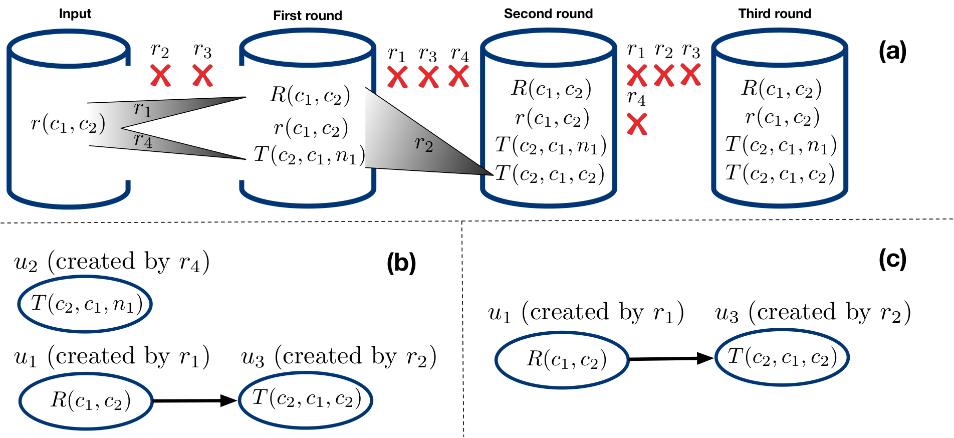
We start our discussion with a simple example to describe how the chase works, its inefficiencies, and how they can be overcome with TGs. For the moment, we give only an intuitive description of some key concepts to aid the understanding of the main ideas. In the following sections, we will provide a formal description.

The chase works in rounds during which it executes the rules over the facts that are currently in the KB. In most chase variants, the execution of a rule involves three steps: retrieving all the facts that instantiate the premise of the rule, then, checking whether the facts to be derived logically hold in the KB and finally, adding them to the KB if they do.

The above steps expose two inefficiencies of the chase. The first is that of incurring in the cost of deriving the same or logically redundant facts.

The second inefficiency that is exposed is that of suboptimally executing the rules themselves: when computing the facts instantiating the premise of a rule, the chase considers all facts currently in the KB even the ones that cannot instantiate the premise of the rule.

The root of these inefficiencies is that the chase, in each round, considers the entire KB as a source for potential derivations, with only SNE as means to avoid some redundant derivations. If we were able to “guide” the execution of the rules in a more clever way, then we can avoid the inefficiencies stated above.

For instance, consider an alternative execution strategy where $r_{2}$ is executed only over the derivations of $r_{1}$, while $r_{3}$ and $r_{4}$ are not executed at all. This strategy would not face any of the inefficiencies highlighted above, and it can be defined with a graph like the one in Figure 1 (c). Informally, a Trigger Graph (TG) is precisely such a graph-based blueprint to compute the materialization. In the remaining, we will first provide a formal definition of TGs and study their properties. Then, we will show that in some cases we can build a TG that is optimal for any possible set of facts given as input. In other cases, we can still build TGs incrementally. Such TGs allow to avoid redundant computations that will occur with the chase but only with the given input.

Let $\mathsf{Consts}$, $\mathsf{Nulls}$, $\mathsf{Vars}$, and $\mathsf{Preds}$ be mutually disjoint, (countably infinite) sets of constants, nulls, variables, and predicates, respectively. Each predicate $p$ is associated with a non-negative integer ${\mathsf{arity}(p)\geq 0}$, called the arity of $p$. Let $\mathsf{EDP}$ and $\mathsf{IDP}$ be disjoint subsets of $\mathsf{Preds}$ of intensional and extensional predicates, respectively. A term is a constant, a null, or a variable. A term is ground if it is either a constant or a null. An atom $A$ has the form ${p(t_{1},\dots,t_{n})}$, where $p$ is an $n$-ary predicate, and ${t_{1},\dots,t_{n}}$ are terms. An atom $A$ is extensional (resp., intensional), if the predicate of $A$ is in $\mathsf{EDP}$ (resp., $\mathsf{IDP}$). A fact is an atom of ground terms. A base fact is an atom of constants whose predicate is extensional. An instance $I$ is a set of facts (possibly comprising null terms). A base instance $B$ is a set of base facts.

A rule is a first-order formula of the form

where, $P$ is an intensional predicate and for all $1\leq i\leq n$, $\mathbf{X}_{i}\subseteq\mathbf{X}$ and $\mathbf{Y}_{1}\subseteq\mathbf{Y}$ ($\mathbf{X}_{i}$ and $\mathbf{Y}_{i}$ might be empty). We assume w.l.o.g. that the body of a rule includes only extensional predicates or intensional predicates. We will denote extensional predicates with lowercase letters, while intensional predicates with uppercase letters. Quantifiers are commonly omitted. The left-hand and the right-hand side of a rule $r$ are its body and head, respectively, and are denoted by $\mathsf{body}(r)$ and $\mathsf{head}(r)$. A rule is Datalog if it has no existentially quantified variables, extensional if $\mathsf{body}(r)$ includes only extensional atoms, and linear if it has a single atom in its body.

A program is a set of rules. A knowledge base (KB) is a pair ${(P,B)}$ with $P$ a program and $B$ a base instance.

Symbol $\models$ denotes logical entailment, where sets of atoms and rules are viewed as first-order theories. Symbol $\equiv$ denotes logical equivalence, i.e., logical entailment in both directions.

A term mapping $\sigma$ is a (possibly partial) mapping of terms to terms; we write ${\sigma=\{t_{1}\mapsto s_{1},\dots,t_{n}\mapsto s_{n}\}}$ to denote that ${\sigma(t_{i})=s_{i}}$ for ${1\leq i\leq n}$. Let $\alpha$ be a term, an atom, a conjunction of atoms, or a set of atoms. Then $\sigma(\alpha)$ is obtained by replacing each occurrence of a term $t$ in $\alpha$ that also occurs in the domain of $\sigma$ with $\sigma(t)$ (i.e., terms outside the domain of $\sigma$ remain unchanged). A substitution is a term mapping whose domain contains only variables and whose range contains only ground terms. For two sets, or conjunctions, of atoms $\mathcal{A}_{1}$ and $\mathcal{A}_{2}$, a term mapping $\sigma$ from the terms occurring in $\mathcal{A}_{1}$ to the terms occurring in $\mathcal{A}_{2}$ is said to be a homomorphism from $\mathcal{A}_{1}$ to $\mathcal{A}_{2}$ if the following hold: (i) $\sigma$ maps each constant in its domain to itself, (ii) $\sigma$ maps each null in its domain to ${\mathsf{Consts}\cup\mathsf{Nulls}}$ and (iii) for each atom $A\in\mathcal{A}_{1}$, ${\sigma(A)\in\mathcal{A}_{2}}$. We denote a homomorphism $\sigma$ from $\mathcal{A}_{1}$ into $\mathcal{A}_{2}$ by $\sigma:\mathcal{A}_{1}\to\mathcal{A}_{2}$.

It is known that, for two sets of facts $\mathcal{A}_{1}$ and $\mathcal{A}_{2}$, there exists a homomorphism from $\mathcal{A}_{1}$ into $\mathcal{A}_{2}$ iff ${\mathcal{A}_{2}\models\mathcal{A}_{1}}$ (and hence, there exists a homomorphism in both ways iff $\mathcal{A}_{1}\equiv\mathcal{A}_{2}$). When $\mathcal{A}_{1}$ and $\mathcal{A}_{2}$ are null-free instances, ${\mathcal{A}_{2}\models\mathcal{A}_{1}}$ iff ${\mathcal{A}_{1}\subseteq\mathcal{A}_{2}}$ and ${\mathcal{A}_{2}\equiv\mathcal{A}_{1}}$ iff ${\mathcal{A}_{1}=\mathcal{A}_{2}}$.

For a set of two or more atoms ${\mathcal{A}=\{A_{1},\dots,A_{n}\}}$ a most general unifier (MGU) $\mu$ for $\mathcal{A}$ is a substitution so that: (i) ${\mu(A_{1})=\dots=\mu(A_{n})}$; and (ii) for each other substitution $\sigma$ for which ${\sigma(A_{1})=\dots=\sigma(A_{n})}$, there exists a $\sigma^{\prime}$ such that ${\sigma=\sigma^{\prime}\circ\mu}$ [5].

Consider a rule $r$ of the form (1) and an instance $I$. A trigger for $r$ in $I$ is a homomorphism from the body of $r$ into $I$. We denote by $h_{s}$ the extension of a trigger $h$ mapping each ${Z\in\mathbf{Z}}$ into a unique fresh null. A rule $r$ holds or is satisfied in an instance $I$, if for each trigger $h$ for $r$ in $I$, there exists an extension $h^{\prime}$ of $h$ to a homomorphism from the head of $r$ into $I$. A model of a KB ${(P,B)}$ is a set ${I\supseteq B}$, such that each ${r\in P}$ holds in $I$. A KB may admit infinitely many different models. A model $M$ is universal, if there exists a homomorphism from $M$ into every other model of ${(P,B)}$. A program $P$ is Finite Expansion Set ($\emph{FES}$), if for each base instance $B$, ${(P,B)}$ admits a finite universal model.

A conjunctive query (CQ) is a formula of the form ${Q(X_{1},\dots,X_{n})\leftarrow\bigwedge_{i=1}^{m}A_{i}}$, where $Q$ is a fresh predicate not occurring in $P$, $A_{i}$ are null-free atoms and each $X_{j}$ occurs in some $A_{i}$ atom. We usually refer to a CQ by its head predicate. We refer to the left-hand and the right-hand side of the formula as the head and the body of the query, respectively. A CQ is atomic if its body consists of a single atom. A Boolean CQ (BCQ) is a CQ whose head predicate has no arguments. A substitution $\sigma$ is an answer to $Q$ on an instance $I$ if the domain of $\sigma$ is precisely its head variables, and if $\sigma$ can be extended to a homomorphism from ${\bigwedge_{i}A_{i}}$ into $I$. We often identify $\sigma$ with the $n$-tuple ${(\sigma(X_{1}),\ldots,\sigma(X_{n}))}$. The output of $Q$ on $I$ is the set $Q(I)$ of all answers to $Q$ on $I$. The answer to a BCQ $Q$ on an instance $I$ is true, denoted as ${I\models Q}$, if there exists a homomorphism from $\bigwedge_{i=1}A_{i}$ into $I$. The answer to a BCQ $Q$ on a KB $(P,B)$ is true, denoted as ${(P,B)\models Q}$, if ${M\models Q}$ holds, for each model $M$ of $(P,B)$. Finally, a CQ $Q_{1}$ is contained in a CQ $Q_{2}$, denoted as ${Q_{1}\subseteq Q_{2}}$, if for each instance $I$, each answer to $Q_{1}$ on $I$ is in the answers to $Q_{2}$ on $I$ [20].

The chase refers to a family of techniques for repairing a base instance $B$ relative to a set of rules $P$ so that the result satisfies the rules in $P$ and contains all base facts from $B$. In particular, the result is a universal model of $(P,B)$, which we can use for query answering [26]. By “chase” we refer both to the procedure and its output.

The chase works in rounds during which it executes one or more rules from the KB. The result of each round ${i\geq 0}$ is a new instance $I^{i}$ (with ${I^{0}=B}$), which includes the facts of all previous instances plus the newly derived facts. The execution of a rule in the $i$-th chase round, involves computing all triggers from the body of $r$ into $I^{i-1}$, then (potentially) checking whether the facts to be derived satisfy certain criteria in the KB and finally, adding to the KB or discarding the derived facts. Different chase variants employ different criteria for deciding whether a fact should be added to the KB or whether to stop or continue the reasoning process [11, 49]. For example, the restricted chase (adopted by VLog and RDFox) adds a fact if there exists no homomorphism from this fact into the KB and terminates when no new fact is added. The warded chase (adopted by Vadalog) replaces homomorphism checks by isomorphism ones [10] and terminates, again, when no new fact is added. The equivalent chase omits any checks and terminates when there is a round $i$ which produces an instance that is logically equivalent to the instance produced in the ${(i-1)}$-th round [24]. Notice that when a KB includes only Datalog rules all chase variants behave the same: a fact is added when it has not been previously derived and the chase stops when no new fact is added to the KB.

Not all chase variants terminate even when the KB admits a finite universal model [24]. The core chase [25] and the equivalent one do offer such guarantees.

For a chase variant, we use $\textit{Ch}^{i}(K)$ or $\textit{Ch}^{i}(P,B)$ to denote the instance computed during the $i$-th chase round and ${\textit{Ch}(P,B)}$ to denote the (possibly infinite) result of the chase. Furthermore, we define the chase graph ${\mathsf{chaseGraph}(P,B)}$ for a KB ${(P,B)}$ as the edge-labeled directed acyclic graph having as nodes the facts in ${\textit{Ch}(P,B)}$ and having an edge from a node $f_{1}$ to $f_{2}$ labeled with rule ${r\in P}$ if $f_{2}$ is obtained from $f_{1}$ and possibly from other facts by executing ${r}$.

In this section, we formally define Trigger Graphs (TGs) and study the class of programs admitting finite instance-independent TGs. First, we introduce the notion of Execution Graphs (EGs). Intuitively, an EG for a program is a digraph stating a “plan” of rule execution to reason via the program. In its general definition, an EG is not required to characterize a plan of reasoning guaranteeing completeness. Particular EGs, defined later, will also satisfy this property.

Figures 1(b) and 1(c) show two EGs for $P_{1}$ from Example 1. Next to each node is the associated rule. Later we show that both EGs are also TGs for $P_{1}$.

Since the nodes of an execution graph are associated with rules of a program, when, in the following, we refer to the head and the body of a node $v$, we actually mean the head and the body of $\mathsf{rule}(v)$. Observe that, by definition, nodes associated with extensional rules do not have entering edges, and nodes $v$ associated with an intensional rule have at most one incoming edge associated with the $j$-th predicate of the body of $v$, i.e., there is at most one node $u$ such that ${u\rightarrow_{j}v}$. The latter might seem counterintuitive as, in a program, the $j$-th predicate in the body of a rule can appear in the heads of many different rules. It is precisely to take into account this possibility that, in an execution graph, more than one node can be associated with the same rule $r$ of the program. In this way, different nodes $v_{1},\dots,v_{q}$ associated with the same rule $r$ can be linked with an edge labeled $j$ to different nodes ${u_{1},\dots,u_{q}}$ whose head’s predicate is the $j$-th predicate of the body of $r$. This models that to evaluate a rule $r$ we might need to match the $j$-th predicate in the body of $r$ with facts generated by the heads of different rules.

We now define some notions on EGs that we will use throughout the paper. For an EG $G$ for a program $P$, we denote by $\nu(G)$ and $\epsilon(G)$ the sets of nodes and edges in $G$. The depth of a node ${v\in\nu(G)}$ is the length of the longest path that ends in $v$. The depth $\mathsf{d}({\textit{G}})$ of $G$ is 0 if $G$ is the empty graph; otherwise, it is the maximum depth of the nodes in $\nu(V)$.

As said earlier, EGs can be used to guide the reasoning process. In the following definition, we formalise how the reasoning over a program $P$ is carried out by following the plan encoded in an EG for $P$. The definition assumes the following for each rule $r$ in $P$: (i) $r$ is of the form ${\forall\mathbf{X}\forall\mathbf{Y}\bigwedge\nolimits_{i=1}^{n}P_{i}(\mathbf{X}_{i},\mathbf{Y}_{i})\to\exists\mathbf{Z}P(\mathbf{Y},\mathbf{Z})}$; and (ii) if $r$ is intensional and is associated with a node $v$ in an EG for $P$, then the EG includes an edge of the form ${u_{i}\rightarrow_{i}v}$, for each ${1\leq i\leq n}$.

TGs are EGs guaranteeing the correct computation of conjunctive query answering.

TGs that depend both on $P$ and $B$ are called instance-dependent, while TGs that depend only on $P$ are called instance-independent. The EGs shown in Figure 1 are both instance-independent TGs for $P_{1}$.

We provide an analysis of the class of programs that admit a finite instance-independent TG denoted as $\emph{FTG}$. Theorem 7 summarizes the relationship between $\emph{FTG}$ and the classes of programs that are bounded ($\emph{BDD}$, [24]), term-depth bounded ($\emph{TDB}$, [39]) and first-order-rewritable ($\emph{FOR}$, [18]).

This result is obtained by showing that if $P$ is $\emph{FTG}$, then it is $\emph{BDD}$ with bound the maximal depth of any instance-independent TG for $P$. If it is $\emph{BDD}$ with bound $k$, then the (finite) EG $G^{k}$, which is described after Definition 9, is a TG for $P$.

If a program is $\emph{FOR}$, then all facts that contain terms of depth at most $k$ are produced in a fixed number of chase steps. Therefore, if it is also $\emph{TDB}$, then all relevant facts in the chase are also produced in a fixed number of steps. Finally, the undecidability of $\emph{FTG}$ follows from the fact that $\emph{FOR}$ and $\emph{FTG}$ coincide for Datalog programs, which are always $\emph{TDB}$. See the appendix for a detailed explanation.

We conclude our analysis by showing that any KB that admits a finite model, also admits a finite instance-dependent TG, as stated in the following statement.

The key insight is that we can build a TG that mimics the chase. Below, we analyze the conditions under which the same rule execution takes place both in the chase and when reasoning over a TG. Based on this analysis we present a technique for computing instance-dependent TGs that mimic breadth-first chase variants.

Consider a rule of the form (1) and assume that the chase over a KB ${(P,B)}$ executes $r$ in some round $k$ by instantiating its body using the facts ${R(\mathbf{c}_{i})}$. Consider now a TG $G$ for ${(P,B)}$. If ${k=1}$, then this rule execution (notice that the rule has to be extensional) takes place in $G$ if there is a node $v$ associated with $r$. Otherwise, if ${k>1}$, then this rule execution takes place in $G$ if the following holds: (i) there is a node $v$ associated with $r$, (ii) each ${R(\mathbf{c}_{i})}$ is stored in some node $u_{i}$ and (iii) there is an incoming edge ${u_{i}\rightarrow_{i}v}$, for each ${1\leq i\leq n}$. We refer to each combination of nodes of depth ${<k}$ whose facts may instantiate the body of a rule $r$ when reasoning over an EG, as $k$-compatible nodes for $r$:

The above ideas are summarized in an iterative procedure, which builds at each step $k$ a graph $G^{k}$:

• •

  (Base step) if ${k=1}$, then for each extensional rule $r$ add to $G^{k}$ a node $v$ associated with $r$.

• •

  (Inductive step) otherwise, for each intensional rule $r$ and each combination of nodes ${(u_{1},\dots,u_{n})}$ from $G^{k-1}$ that is $k$-compatible with $r$, add to $G^{k}$: (i) a fresh node $v$ associated with $r$ and (ii) an edge ${u_{i}\rightarrow_{i}v}$, for each ${1\leq i\leq n}$.

The inductive step ensures that $G^{k}$ encodes each rule execution that takes place in the $k$-th chase round.

So far, we did not specify when the TG computation process stops. When $P$ is Datalog, we can stop when ${G^{k-1}(B)=G^{k}(B)}$. Otherwise, we can employ the termination criterion of the equivalent chase, e.g., ${G^{k-1}(B)\models G^{k}(B)}$, or of the restricted chase.

In the previous section, we outlined a procedure to compute instance-dependent TGs that mimics the chase. Now, we propose an algorithm for computing instance-independent TGs for linear programs.

Our technique is based on two ideas. The first one is that, for each base instance $B$, the result of chasing $B$ using a linear program $P$ is logically equivalent to the union of the instances computed when chasing each single fact in $B$ using $P$.

The second idea is based on pattern-isomorphic facts: facts with the same predicate name and for which there is a bijection between their constants. For example, ${R(1,2,3)}$ is pattern-isomorphic to ${R(5,6,7)}$ but not to ${R(9,9,8)}$. We can see that two different pattern-isomorphic facts will have the same linear rules executed in the same order during chasing. We denote by $\mathcal{H}(P)$ a set of facts formed over the extensional predicates in a program $P$, where no fact ${f_{1}\in\mathcal{H}(P)}$ is pattern isomorphic to some other fact ${f_{2}\in\mathcal{H}(P)}$.

Algorithm 1 combines these two ideas: it runs the chase for each fact in $\mathcal{H}(P)$ then tracks the rule executions and (iii) based on these rule executions it computes a TG. In particular, for each fact $f_{2}$ that is derived after executing a rule $r$ over $f_{1}$, Algorithm 1 will create a fresh node $u$ and associate it with rule $r$, lines 4–6. The mapping $\mu$ associates nodes with rule executions. Then, the algorithm adds edges between the nodes based on the sequences of rule executions that took place during chasing, lines 7–9.

Algorithm 1 is (implicitly) parameterized by the chase variant. The results below are based on the equivalent chase, as it ensures termination for $\emph{FES}$ programs.

Algorithm 1 has a double-exponential overhead.

There are cases where we cannot compute instance-independent TG, e.g., for Datalog programs that are not also in $\emph{FTG}$ class. In such cases, we can still create an instance-dependent TG using the procedure outlined in Section 4. In this section, we present two optimizations to this procedure which avoid redundant computations. These optimizations work with Datalog programs; thus also with non-linear rules.

We implemented Algorithm 1, TG-guided reasoning over a fixed TG (Def. 5) and Algorithm 2 in a new open-source reasoner called GLog. GLog is a fork of VLog [60] that shares the same code for handling the extensional relations while the code for reasoning is entirely novel.

We consider three performance measures: the absolute reasoning runtime, the peak RAM consumption observed at reasoning time, and the total number of triggers. The last measure is added because it reflects the ability of TGs to reduce the number of redundant rule executions and it is robust to most implementation choices.

References

- [1] RDFox public release. https://github.com/dbunibas/chasebench/tree/master/tools/rdfox. Accessed: 2020-11-10.
- [2] S. Abiteboul, R. Hull, and V. Vianu. Foundations of Databases. Addison Wesley, 1995.
- [3] M. Aref, B. ten Cate, T. J. Green, B. Kimelfeld, D. Olteanu, E. Pasalic, T. L. Veldhuizen, and G. Washburn. Design and Implementation of the LogicBlox System. In SIGMOD, pages 1371–1382, 2015.
- [4] P. C. Arocena, B. Glavic, R. Ciucanu, and R. J. Miller. The iBench Integration Metadata Generator. In VLDB, page 108–119, 2015.
- [5] F. Baader and T. Nipkow. Term Rewriting and All That. Cambridge University Press, USA, 1999.
- [6] J. Baget, M. Leclère, M. Mugnier, S. Rocher, and C. Sipieter. Graal: A Toolkit for Query Answering with Existential Rules. In RuleML, 2015.
- [7] J. Baget, M. Leclère, M. Mugnier, and E. Salvat. On rules with existential variables: Walking the decidability line. Artificial Intelligence, 175(9-10):1620–1654, 2011.
- [8] F. Bancilhon, D. Maier, Y. Sagiv, and J. D. Ullman. Magic Sets and Other Strange Ways to Implement Logic Programs. In PODS, pages 1–15, 1986.
- [9] C. Beeri and R. Ramakrishnan. On the Power of Magic. Journal of Logic Programming, 10(3,4):255–299, 1991.
- [10] L. Bellomarini, E. Sallinger, and G. Gottlob. The Vadalog System: Datalog-based Reasoning for Knowledge Graphs. PVLDB, 11(9):975–987, 2018.
- [11] M. Benedikt, G. Konstantinidis, G. Mecca, B. Motik, P. Papotti, D. Santoro, and E. Tsamoura. Benchmarking the chase. In PODS, pages 37–52, 2017.
- [12] M. Benedikt, J. Leblay, and E. Tsamoura. PDQ: Proof-driven query answering over web-based data. In VLDB, page 1553–1556, 2014.
- [13] M. Benedikt, B. Motik, and E. Tsamoura. Goal-driven query answering for existential rules with equality. In AAAI, pages 1761 – 1770, 2018.
- [14] C. Bizer, J. Lehmann, G. Kobilarov, S. Auer, C. Becker, R. Cyganiak, and S. Hellman. DBpedia - A crystallization point for the Web of Data. Journal of Web Semantics, 7(3):154–165, 2009.
- [15] A. Bonifati, I. Ileana, and M. Linardi. Functional Dependencies Unleashed for Scalable Data Exchange. In SSDBM, 2016.
- [16] D. Brickley, R. V. Guha, and B. McBride. Rdf schema 1.1. W3C recommendation, 25:2004–2014, 2014.
- [17] A. Calì, G. Gottlob, and M. Kifer. Taming the infinite chase: Query answering under expressive relational constraints. J. Artif. Int. Res., 48(1):115–174, 2013.
- [18] A. Calì, G. Gottlob, and T. Lukasiewicz. A general Datalog-based framework for tractable query answering over ontologies. Journal of Web Semantics, 14:57–83, 2012.
- [19] D. Calvanese, B. Cogrel, S. Komla-Ebri, R. Kontchakov, D. Lanti, M. Rezk, M. Rodriguez-Muro, and G. Xiao. Ontop: Answering SPARQL queries over relational databases. Semantic Web, 8(3):471–487, 2017.
- [20] A. K. Chandra and P. M. Merlin. Optimal implementation of conjunctive queries in relational data bases. In STOC, pages 77–90, 1977.
- [21] B. Chin, D. von Dincklage, V. Ercegovac, P. Hawkins, M. S. Miller, F. Och, C. Olston, and F. Pereira. Yedalog: Exploring knowledge at scale. In SNAPL, pages 63–78, 2015.
- [22] D. Croft, A. F. Mundo, R. Haw, M. Milacic, J. Weiser, G. Wu, M. Caudy, P. Garapati, M. Gillespie, M. R. Kamdar, et al. The reactome pathway knowledgebase. Nucleic acids research, 42(D1):D472–D477, 2013.
- [23] A. S. d’Avila Garcez, K. Broda, and D. M. Gabbay. Neural-symbolic learning systems: foundations and applications. Perspectives in neural computing. Springer, 2002.
- [24] S. Delivorias, M. Leclère, M. Mugnier, and F. Ulliana. On the k-Boundedness for Existential Rules. In RuleML+RR, pages 48–64, 2018.
- [25] A. Deutsch, A. Nash, and J. B. Remmel. The chase revisited. In PODS, pages 149–158, 2008.
- [26] R. Fagin, P. G. Kolaitis, R. J. Miller, and L. Popa. Data exchange: semantics and query answering. Theoretical Computer Science, 336(1):89–124, 2005.
- [27] F. Geerts, G. Mecca, P. Papotti, and D. Santoro. That’s All Folks! LLUNATIC Goes Open Source. In VLDB, page 1565–1568, 2014.
- [28] G. Gottlob, G. Orsi, and A. Pieris. Ontological query answering via rewriting. In ADBIS, pages 1–18, 2011.
- [29] G. Gottlob, G. Orsi, and A. Pieris. Query Rewriting and Optimization for Ontological Databases. ACM TODS, 39(3):25:1–25:46, 2014.
- [30] Y. Guo, Z. Pan, and J. Heflin. LUBM: A benchmark for OWL knowledge base systems. Journal of Web Semantics, 3(2-3), 2011.
- [31] J. Hoffart, F. Suchanek, K. Berberich, and G. Weikum. Yago2: A spatially and temporally enhanced knowledge base from wikipedia. Artificial Intelligence, 194:28–61, 2013.
- [32] A. Hogan, E. Blomqvist, M. Cochez, C. d’Amato, G. de Melo, C. Gutierrez, J. E. L. Gayo, S. Kirrane, S. Neumaier, A. Polleres, R. Navigli, A.-C. N. Ngomo, S. M. Rashid, A. Rula, L. Schmelzeisen, J. Sequeda, S. Staab, and A. Zimmermann. Knowledge Graphs. arXiv:2003.02320 [cs], 2020. arXiv: 2003.02320.
- [33] P. Hu, B. Motik, and I. Horrocks. Modular materialisation of datalog programs. In AAAI, pages 2859–2866, 2019.
- [34] P. Hu, J. Urbani, B. Motik, and I. Horrocks. Datalog Reasoning over Compressed RDF Knowledge Bases. In CIKM, pages 2065–2068, 2019.
- [35] N. Konstantinou, M. Koehler, E. Abel, C. Civili, B. Neumayr, E. Sallinger, A. A. Fernandes, G. Gottlob, J. A. Keane, L. Libkin, and N. W. Paton. The VADA Architecture for Cost-Effective Data Wrangling. In SIGMOD, pages 1599–1602, 2017.
- [36] B. Kruit, P. A. Boncz, and J. Urbani. Extracting novel facts from tables for knowledge graph completion. In ISWC, pages 364–381, 2019.
- [37] B. Kruit, H. He, and J. Urbani. Tab2know: Building a knowledge base from tables in scientific papers. In ISWC, pages 349–365. Springer, 2020.
- [38] M. Leclère, M. Mugnier, M. Thomazo, and F. Ulliana. A Single Approach to Decide Chase Termination on Linear Existential Rules. In ICDT, pages 18:1–18:19, 2019.
- [39] M. Leclère, M. Mugnier, and F. Ulliana. On bounded positive existential rules. In DL, 2016.
- [40] J. Lee, T. Hwang, J. Park, Y. Lee, B. Motik, and I. Horrocks. A Context-Aware Recommendation System for Mobile Devices. In ISWC, pages 380–382, 2020.
- [41] L. Ma, Y. Yang, Z. Qiu, G. Xie, Y. Pan, and S. Liu. Towards a complete OWL Ontology Benchmark. In ESWC, pages 125–139, 2006.
- [42] D. Maier, A. O. Mendelzon, and Y. Sagiv. Testing implications of data dependencies. ACM Transactions on Database Systems, 4(4):45–5469, 1979.
- [43] M. Meier. The backchase revisited. VLDB J., 23(3):495–516, 2014.
- [44] B. Motik, B. C. Grau, I. Horrocks, Z. Wu, A. Fokoue, C. Lutz, et al. OWL 2 web ontology language profiles. W3C recommendation, 27:61, 2009.
- [45] B. Motik, Y. Nenov, R. Piro, I. Horrocks, and D. Olteanu. Parallel Materialisation of Datalog Programs in Centralised, Main-Memory RDF Systems. In AAAI, pages 129–137, 2014.
- [46] W. E. Moustafa, V. Papavasileiou, K. Yocum, and A. Deutsch. Datalography: Scaling datalog graph analytics on graph processing systems. In IEEE International Conference on Big Data, pages 56–65, 2016.
- [47] Y. Nenov, R. Piro, B. Motik, I. Horrocks, Z. Wu, and J. Banerjee. RDFox: A Highly-Scalable RDF Store. In ISWC, pages 3–20, 2015.
- [48] N. Noy, Y. Gao, A. Jain, A. Narayanan, A. Patterson, and J. Taylor. Industry-scale Knowledge Graphs: Lessons and Challenges. Commun. ACM, 62(8):36–43, July 2019.
- [49] A. Onet. The chase procedure and its applications in data exchange. In DEIS, pages 1–37, 2013.
- [50] R. Pichler and V. Savenkov. DEMo: Data Exchange Modeling Tool. In VLDB, pages 1606–1609, 2009.
- [51] S. Rahtz, A. Dutton, D. Kurtz, G. Klyne, A. Zisserman, and R. Arandjelovic. CLAROS—Collaborating on Delivering the Future of the Past. In DH, pages 355–357, 2011.
- [52] Y. Sagiv and M. Yannakakis. Equivalences among relational expressions with the union and difference operators. Journal of the ACM, 27(4):633–655, 1980.
- [53] D. Sereni, P. Avgustinov, and O. de Moor. Adding Magic to an Optimising Datalog Compiler. In SIGMOD, pages 553–566, 2008.
- [54] J. Subercaze, C. Gravier, J. Chevalier, and F. Laforest. Inferray: Fast in-Memory RDF Inference. Proceedings of the VLDB Endowment, 9(6):468–479, 2016.
- [55] K. T. Tekle and Y. A. Liu. More Efficient Datalog Queries: Subsumptive Tabling Beats Magic Sets. In SIGMOD, pages 661–672, 2011.
- [56] E. Tsamoura, V. Gutiérrez-Basulto, and A. Kimmig. Beyond the Grounding Bottleneck: Datalog Techniques for Inference in Probabilistic Logic Programs. In AAAI, pages 10284–10291, 2020.
- [57] J. Urbani and C. Jacobs. Adaptive Low-level Storage of Very Large Knowledge Graphs. In WWW, pages 1761–1772, 2020.
- [58] J. Urbani, C. Jacobs, and M. Krötzsch. Column-Oriented Datalog Materialization for Large Knowledge Graphs. In AAAI, pages 258–264, 2016.
- [59] J. Urbani, S. Kotoulas, J. Maassen, F. van Harmelen, and H. Bal. OWL Reasoning with WebPIE: Calculating the Closure of 100 Billion Triples. In ESWC, pages 213–227, 2010.
- [60] J. Urbani, M. Krötzsch, C. Jacobs, I. Dragoste, and D. Carral. Efficient Model Construction for Horn Logic with VLog. In IJCAR, pages 680–688, 2018.
- [61] Y. Zhou, B. Cuenca Grau, I. Horrocks, Z. Wu, and J. Banerjee. Making the Most of your Triple Store: Query Answering in OWL 2 using an RL Reasoner. In WWW, pages 1569–1580, 2013.
Appendix A Addtional experimental results