On the Global Optimality of Whittle’s index policy for minimizing the age of information

We consider a time-slotted system with one base station, $M$ uncorrelated channels, and $N$ users ($N>M$). Time is considered to be normalized to the slot duration (i.e, $t=1,2,\ldots$). We suppose that any of the $M$ channels can be allocated to at most one user. Hence, at most $M$ users will be able to transmit in each time slot $t$. If a user is scheduled at time $t$, it generates a fresh new packet and sends it to the base station. This packet is successfully decoded by the base station at time $t+1$ with a certain success probability. We consider that if a decoding error takes place, the packet is discarded (i.e., users are not equipped with buffers). In practice, users may share similar channel conditions. Accordingly, we suppose that the users can be partitioned into $K=2$ different classes such that users within the same class share the same decoding success probability. In other words, each user $i$ belonging to class $k\in\{1,2\}$ has a decoding success probability $p_{k}$, which is assumed to be known by the scheduler. We let $\gamma_{k}$ be the proportion of users belonging to class $k$. To that end, the following always holds: $\gamma_{1}+\gamma_{2}=1$.

A scheduling policy $\pi$ is defined as a sequence of actions $\pi=(\boldsymbol{a}^{\pi}(0),\boldsymbol{a}^{\pi}(1),\ldots)$ where
$\boldsymbol{a}^{\pi}(t)=(a_{1}^{1,\pi}(t),a_{2}^{1,\pi}(t),\ldots,a_{\gamma_{1}N}^{1,\pi}(t),a_{1}^{2,\pi}(t),a_{2}^{2,\pi}(t),\ldots,a_{\gamma_{2}N}^{2,\pi}(t))$ is a binary vector such that $a_{i}^{k,\pi}(t)=1$ if user $i$ of class $k$ is scheduled at time $t$. We also let the binary random variable $c_{i}^{k}(t)$ denote the channel state of user $i$ of class $k$ such that $c_{i}^{k}(t)=1$ if no decoding error takes place. As per our system model, we always have $\Pr(c_{i}^{k}(t)=1)=p_{k}$ and $\Pr(c_{i}^{k}(t)=0)=1-p_{k}$ for any user $i$ of class $k$. We let $B_{i}^{k,\pi}(t)$ denote the time-stamp of the freshest packet delivered by user $i$ of class $k$ to the base station at time $t$ under the scheduling policy $\pi$. The age of information, or simply the age, of user $i$ of class $k$ is defined as [1]:

By taking into account the variables defined, the age of this user under policy $\pi$ evolves as follows:

We let $\boldsymbol{s}^{\pi}(t)$ denote the vector of all users’ age $\boldsymbol{s}^{\pi}(t)=(s_{1}^{1,\pi}(t),\cdots,s_{\gamma_{1}N}^{1,\pi}(t),s_{1}^{2,\pi}(t),\cdots,s_{\gamma_{2}N}^{2,\pi}(t))$ under policy $\pi$. With all these notations in mind, we can formulate the optimization problem that we focus on in our paper.

In this paper, we are interested in minimizing the total expected average age of information of the network under the constraint on the number of users scheduled at each time slot $t$. The latter must be less than the total number of channels $\alpha N$ where $\alpha$ is equal to $\frac{M}{N}$. We let $\Pi$ denote the set of all causal scheduling policies in which the scheduling decisions are made based on the history and current states of the system. To that end, and given an initial system state $\boldsymbol{s}(0)=(s_{1}^{1}(0),\cdots,s_{\gamma_{1}N}^{1}(0),\cdots,s_{1}^{K}(0),\cdots,s_{\gamma_{K}N}^{K}(0))$, our problem can be formulated as follows:

This problems belongs to the family of RMAB problems, which are generally difficult to solve optimally (see Papadimitriou et al. [26]). For this reason, one should aim to develop a well-performing sub-optimal policy. As it has been mentioned, the low-complexity scheduling policy that we are interested in throughout this paper is the Whittle’s index policy. To establish this policy and derive the Whittle’s indices expressions, one has to follow the steps below:

1. 1.

   Provide a relaxed version of the original problem and tackle it through a Lagrangian approach.

2. 2.

   Prove the indexability property of the problem and derive the Whittle’s index expressions.

As previously mentioned, these steps have been carried out in previous works by the authors in [15]. For completeness, and as we will use these steps later in our optimality analysis, we report them along with the main results of [15] in the following section.

The first step toward establishing the Whittle’s index policy consists of relaxing the constraint on the number of scheduled users of the problem in (5). Specifically, instead of having the constraint satisfied at each time slot, we consider that it has to be satisfied on average. Therefore, the relaxed problem can be formulated as follows:

To study this problem, one has to introduce a Lagrangian approach to transform the problem into an unconstrained one as will be detailed in the sequel.

To circumvent the difficulty of studying the constrained problem in (6), a Lagrangian approach has to be adopted. In particular, let us denote by $\lambda\geq 0$ the Lagrangian parameter. For a fixed $\lambda$, the Lagrangian function of the relaxed problem is:

Based on the dual approach, the next step consists of finding the policy $\pi$ that minimizes $F(\lambda,\pi)$. Note that the term $\frac{1}{T}\sum_{t=0}^{T-1}\sum_{k=1}^{K}\sum_{i=1}^{{\gamma_{k}}N}\lambda\alpha$, which is equal to $N\lambda\alpha$, doesn’t depend on $\pi$. Therefore, the policy that minimizes the above function $F(\lambda,\pi)$ also minimizes the following function:

Then, we can formulate the dual problem as follows:

To solve the problem in (9), it can be shown that this $N$-dimensional problem can be decomposed into $N$ one-dimensional problems that can be solved independently [15]. Therefore, we can drop the $i$ and $k$ indices from (8) and simply investigate the following one-dimensional problem:

It turns out that the above one dimensional problem can be cast into an infinite horizon average cost Markov Decision Process (MDP) that is defined as follows:

• •

  States: The state of the MDP at time $t$ is the age of the user $s(t)$ that can take any integer value strictly higher than $0$. Therefore, the considered state space is countable and infinite.

• •

  Actions: The action at time $t$, denoted by $a(t)$, indicates if a transmission is attempted (value $1$) or the user remains idle (value $0$).

• •

  Transitions probabilities: The transitions probabilities between the different states have been previously detailed in Section II.

• •

  Cost: The cost function at time $t$ is designated by $C(s(t),a(t))=s(t)+\lambda a(t)$.

To solve this MDP, the authors in [15] have leveraged the Bellman equation and studied the characteristics of the value function involved. Based on the particularity of the value function, the following result was found:

The above results tell us that there exists an integer $l_{k}\in\mathbb{N}^{*}$ such that by only letting users of class $k$ with an age larger or equal to $l_{k}$ to transmit, we attain the optimal operating point of (10). These results are pivotal to proceed with establishing the Whittle’s index policy.

To proceed toward our goal, one has to analyze the behavior of the MDP when a threshold policy is adopted. To that end, we note that for any fixed threshold $n$, the MDP can be modeled through a Discrete Time Markov Chain (DTMC) where:

• •

  The state is the age $s(t)$.

• •

  For any state $s(t)<n$, the user is idle. On the other hand, when $s(t)\geq n$, the user is scheduled.

The DTMC is reported in Fig. 1.

To be able to prove the indexability property and find the Whittle’s index expression, one has to find the average objective function in (10) when a threshold policy is adopted. To that end, we provide the following propositions.

The next step consists of calculating the average objective function in (10) when a threshold policy is employed.

Using the stationary distribution, and the average cost, one can then prove the indexability property of the problem, which ensures the existence of the Whittle’s indices. Before providing these results, we first lay out the definition of the aforementioned property.

The indexability property for the problem in (10) was established by the authors in [15]. With the Whittle’s indices ensured to exist, one can then leverage the stationary distribution and the average cost reported in Proposition 2 and 3 to derive the Whittle’s index expressions as previously done in [15] and [21].

With the Whittle’s index expression derived, we can now establish the Whittle’s index scheduling policy. This can be summarized in the following algorithm description.

Although the above scheduling policy is easy to implement, it remains sub-optimal. Accordingly, characterizing its performance compared to the optimal policy is important. Equipped with the above results and notations, we can now tackle the main issue that we aim to address in our paper: the asymptotic optimality of this policy.

To be able to prove the asymptotic optimality of the Whittle’s index policy, one has to compare its performance to the optimal policy that solves (5). However, as previously explained, the optimal policy of (5) is not known. To circumvent this, and to have a benchmark performance to compare to, we note that the following always holds:

where $\frac{C^{WIP,N}}{N}$ is the average age per-user under the Whittle’s index policy, $\frac{C^{OP,N}}{N}$ is the optimal expected average age per-user of the original problem (5), and $\frac{C^{RP,N}}{N}$ is the optimal average age per-user of the relaxed problem (6). Thus, in order to show the asymptotic optimality, it is sufficient to prove that for a large number of users $N$, $\frac{C^{WIP,N}}{N}$ converges to $\frac{C^{RP,N}}{N}$. To that end, the next task is to find an expression of $C^{RP}=\frac{C^{RP,N}}{N}$. For this purpose, we provide the following proposition.

Thanks to this proposition, we can conclude that the optimal per-user cost of the relaxed problem has the following expression:

By leveraging these results, we can proceed with characterizing the performance of the Whittle’s index policy.

This section constitutes the main contribution of the paper where we show the asymptotic optimality of the Whittle’s index policy. The idea is to show that the performance of this policy converges to $C^{RP}$ when $N$ is large and the ratio $\alpha=\frac{M}{N}$ is kept constant.

We let $Z_{i}^{k,N}(t)$ denote the proportion of users belonging to class $k$ in state $i$ at time $t$. In other words, it denotes the ratio of the number of users in class $k$ having an age equal to $i$ to the total number of users $N$. We have that $\boldsymbol{Z}^{N}(t)=(Z^{1,N}(t),.....,Z^{K,N}(t))$ with $Z^{k,N}(t)=(Z_{1}^{k,N}(t),......,Z^{k,N}_{m^{k}(t)}(t))$, where $m^{k}(t)$ is the highest state at time $t$ in class $k$ and $\sum_{i=0}^{m^{k}(t)}Z_{i}^{k,N}(t)=\gamma_{k}$ for each class $k$. We also denote by $\boldsymbol{z}^{*}$ the proportion corresponding to the optimal policy of the relaxed problem. Thus, the elements of the vector $\boldsymbol{z}^{*}$ are exactly the set $\{\gamma_{k}(\theta u_{k}^{l_{k}^{1}}(i)+(1-\theta)u_{k}^{l_{k}^{2}}(i))\}_{1\leq k\leq K\atop 1\leq i}$ where $i$ and $k$ refer to the user $i$ and class $k$ respectively. This can be easily concluded from the results previously laid out in eq. (17).

In the sequel, we will establish the global optimality for two different classes of users where $p_{1}$ and $p_{2}$ are the successful transmission probabilities of class $1$ and $2$ respectively ($p_{1}>p_{2}$). In order to prove that, we show that when the Whittle’s index policy is adopted, $\boldsymbol{Z}^{N}(t)$ converges in probability to $\boldsymbol{z}^{*}$ when $N$ and $t$ are very large. To that extent, we follow the steps below:

• •

  We show that the fluid approximation of $\boldsymbol{Z}^{N}(t)$, denoted by $\boldsymbol{z}(t)$, converges to $\boldsymbol{z}^{*}$. Such a convergence has been proven in previous works under restrictive mathematical assumptions that can only be verified numerically [22]. We escape these assumptions as we will detail in the following.

• •

  Since the relation between $\boldsymbol{z}(t+1)$ and $\boldsymbol{z}(t)$ is not linear, our approach to establish the convergence of $\boldsymbol{z}(t)$ involves two terms: $\alpha_{1}(t)$ and $\alpha_{2}(t)$. These two proportions are nothing but the scheduled proportion at time $t$ of class $1$ and $2$, respectively. Note that we always have $\alpha_{1}(t)+\alpha_{2}(t)=\alpha$. Based on Lemma 1, we show that for a large enough time $t$, there exists $T_{t}$ such that we can find a partial relation between each element of the vector $\boldsymbol{z}(t+T_{t})$ and terms of the sequence $\{\alpha_{k}(t^{\prime})\}_{k=1,2\atop t^{\prime}\leq t+T_{t}}$. More precisely, we prove that for $T_{t}$, we can express each proportion that is not scheduled at time $t+T_{t}$ in function of one term of $\{\alpha_{k}(t^{\prime})\}_{k=1,2\atop t^{\prime}\leq t+T_{t}}$. This allows us to obtain $1-\alpha$ as a linear combination between the terms of $\{\alpha_{k}(t^{\prime})\}_{k=1,2\atop t^{\prime}\leq t+T_{t}}$ at time $t+T_{t}$.

• •

  Subsequently, we introduce in Definition 3, $T_{\max}$ that satisfies these two following properties proven in Propositions 7 and 8 using Lemma 2: the Whittle’s index alternates between the two classes from state $1$ to $T_{\max}$ under a given assumption on $\alpha$; the instantaneous thresholds $l_{1}(.)$ and $l_{2}(.)$ are bounded by $T_{\max}$ at time $t+T_{t}$.

• •

  Based on that, we derive the relation between the instantaneous thresholds at time $t+T_{t}$ in Proposition 9. Taking as initial time $t+T_{t}=T_{0}$, we show by induction in Proposition 10 that, for all $T\geq T_{0}$, the instantaneous thresholds are less than $T_{\max}$ and that all none scheduled proportions can be expressed in function of terms of the sequence $\{\alpha_{k}(t^{\prime})\}_{k=1,2\atop t^{\prime}\leq T}$. Next, we define for each class $k$ a vector $A_{k}(T)$ composed by $\alpha_{k}(T)$ (the scheduled proportion at time $T$) plus the finite subset of the sequence $\{\alpha_{k}(t^{\prime})\}_{t^{\prime}\leq T}$ such that for all proportion of users in class $k$ at a given state at time $T$ that is not scheduled can be expressed by one element belonging to this subset. After that, we provide the relation between the elements of the vectors $A_{k}(T)$ and $A_{k}(T+1)$ in Propositions 11 and 12

• •

  As was mentioned in Introduction, our proof is based on Cauchy criterion which states that in the real number space $\mathbb{R}$, a given sequence $h(T)$ is convergent if and only if its terms become closer together as $T$ increases. To that extent, we show that the elements of the vector $A_{k}(\cdot)$ which are nothing but the terms of the sequence $\alpha_{k}(\cdot)$ are getting closer when $T$ increases. For that purpose, we prove that the highest and the smallest element of $A_{k}(T)$ converge to the same limit when $T$ grows. To that end, we start by establishing the convergence of the highest and the smallest element of $A_{k}(T)$ in Theorem 1. Then, we demonstrate by contradiction that the highest and the smallest element of $A_{k}(T)$ must converge to the same limit in Proposition 13. This last result implies that $\alpha_{k}(t)$ converges when $t$ scales. In light of that fact, we prove that $\boldsymbol{z}(t)$ converges to $\boldsymbol{z}^{*}$ in Proposition 14. Finally, using Kurth theorem, we show in Proposition 15 that $\boldsymbol{Z}^{N}(t)$ converges to $\boldsymbol{z}^{*}$ in probability. And finally we establish in Proposition 16 the convergence of $\frac{C^{WIP,N}}{N}$ to $C^{RP}$.

With the steps of our approach clarified, we can proceed with introducing the fluid limit approximation. The fluid limit technique consists of analyzing the evolution of the expectation of $\boldsymbol{Z}^{N}(t)$ under the Whittle’s index policy. For that, we define the vector $\boldsymbol{z}(t)$ as follows:

This above equation reveals to us that we have a sequence $\boldsymbol{z}(t)$ defined by recurrence for a fixed initial state $\boldsymbol{z}(0)$ that we should study its behavior when $t$ is very large. Hence, we end up with a function $\boldsymbol{z}(t)$ that depends on two variables, $t$ and the initial value $\boldsymbol{z}(0)$. To that extent, our aim is to prove that $\boldsymbol{z}(t)$ converges to $\boldsymbol{z}^{*}$ regardless of the initial state $\boldsymbol{z}(0)$. We let $\boldsymbol{z}(t)=(\boldsymbol{z}^{1}(t),.....,\boldsymbol{z}^{K}(t))$ with $\boldsymbol{z}^{k}(t)=(z_{1}^{k}(t),......,z^{k}_{m^{k}(t)}(t))$ where $z_{i}^{k}(t)$ is the expected proportion of users at state $i$ in class $k$ at time $t$ with respect to the equation (18). Accordingly we have that $\sum_{i=0}^{m^{k}(t)}z_{i}^{k}(t)=\gamma_{k}$ for each class $k$.

One can notice that $\boldsymbol{z}^{*}$ is a particular vector with respect to the equation (18).

According to this proposition, it is sufficient to show that $\boldsymbol{z}(t)$ converges starting from any initial state $\boldsymbol{z}(0)$, as the only eventual finite limit of $\boldsymbol{z}(t)$ when $t$ tends to $+\infty$ is the fixed point of the equation (18), $\boldsymbol{z}^{*}$.

In the following, we prove that the fluid approximation vector of $\boldsymbol{Z}^{N}(t)$, $\boldsymbol{z}(t)$ under the Whittle Index Policy converges starting from any initial state. We prove this result for 2 different classes of users where $p_{1}$ and $p_{2}$ are the successful transmission probabilities of the class 1 and 2 respectively ($p_{1}>p_{2}$), given a sufficient condition on $\alpha$. Throughout this section, we denote by $w_{1}(n)$ and $w_{2}(n)$, the Whittle’s index, whose expression is given in Proposition 4, of state $n$ in class 1 and class 2 respectively. We need to prove that $z_{i}^{k}(t)$ converges for each state $i$ in class $k$.

Now, focusing on the Whittle index policy, we can see it as an instantaneous threshold policy for each class, where the thresholds vary over time $t$. Moreover, under the Whittle index policy, the proportion of users that are scheduled at each time slot $t$ is fixed and equals to $\alpha$ since the number of scheduled users at each time slot $t$ is $\alpha N$. This proportion $\alpha$ contains the users with the highest Whittle index values. In that respect, we define $\alpha_{1}(t)$ and $\alpha_{2}(t)$ the proportion of users in class 1 and class 2 respectively at time $t$ with the highest Whittle index values such that $\alpha_{1}(t)+\alpha_{2}(t)=\alpha$. The remaining proportion of users which are not scheduled at each time slot $t$, which is equal to $1-\alpha$, contains the users with the smallest Whittle index values. Now, regarding this proportion, we give its decomposition into proportions of users at different states in different classes. Denoting by $l_{1}(t)$ and $l_{2}(t)$ at time $t$ the instantaneous threshold integers under Whittle index policy, then there exists two real values between 0 and 1, $\beta(t)$ and $\gamma(t)$, with $\gamma(t)=1$ and $0<\beta(t)\leq 1$, or $0<\gamma(t)\leq 1$ and $\beta(t)=1$, such that:

and $\{z_{i}^{1}\}_{1\leq i\leq l_{1}(t)}\cup\{z_{i}^{2}\}_{1\leq i\leq l_{2}(t)}$ is exactly the set $\{z_{i}^{k}:w_{k}(i)\leq\max(w_{1}(l_{1}(t),w_{2}(l_{2}(t))\}$.

In paper [21], in order to prove the convergence of $\boldsymbol{z}(t)$, the authors assume that $\boldsymbol{z}(0)$ is within a precise neighborhood of $\boldsymbol{z}^{*}$ and they consider that the number of states is finite. These assumptions allow them to find an easy linear relation between $\boldsymbol{z}(t)$ and $\boldsymbol{z}(t+1)$ ($\boldsymbol{z}(t+1)=\boldsymbol{Q}\boldsymbol{z}(t)+\boldsymbol{c}$ see [21, Section IV-C]), and then deduce the convergence of $\boldsymbol{z}$ by establishing that the spectral value of $\boldsymbol{Q}$ is less strictly than one. In our case, as we aim to prove the convergence of $\boldsymbol{z}$ from any initial state, the relation between $\boldsymbol{z}(t+1)$ and $\boldsymbol{z}(t)$ is as follows

This equation is not linear which makes studying the evolution of $\boldsymbol{z}(\cdot)$ a hard task. Moreover, as the number of state is infinite, then the dimensions of $\boldsymbol{z}(t)$ varies per time. Therefore, the matrix $\boldsymbol{Q}(\boldsymbol{z}(t))$ is not square. Hence we can not apply the same method as in [21] since the spectral values are not defined for a non square matrix. For these reasons, we proceed differently than [21]. Our method consists in fact on expressing each proportion $z_{i}^{k}(t)$ that belongs to a non scheduled users’ proportion at time $t$ in function of a term of $\alpha_{k}(\cdot)$ at a given time less than $t$. By this way, we will obtain a part of the vector $\boldsymbol{z}(t)$ in function of $\{\alpha_{k}(t^{\prime})\}_{\begin{subarray}{c}t^{\prime}\leq t,\\ k\in\{0,1\}\end{subarray}}$, and the sum of the other part equal to $\alpha$. Then, we show that $\alpha_{k}(\cdot)$ converges for $k=1,2$. We will see later that it is sufficient to show that $\alpha_{k}(\cdot)$ converges in order to conclude for the convergence of $\boldsymbol{z}(\cdot)$. To find the partial relation between $\boldsymbol{z}(t)$ and $\{\alpha_{k}(t^{\prime})\}_{\begin{subarray}{c}t^{\prime}\leq t\\ k\in\{0,1\}\end{subarray}}$, we prove the following lemma.

According to Lemma 1, after scheduling under the Whittle’s Index Policy, we get at time $t+1$, a proportion of $p_{1}\alpha_{1}(t)$ of users at state 1 in class 1 and $p_{2}\alpha_{2}(t)$ of users at state 1 in class 2 respectively (i.e. $z_{1}^{1}(t+1)=p_{1}\alpha_{1}(t)$ and $z_{1}^{2}(t+1)=p_{2}\alpha_{2}(t)$).
According to the same lemma, at time $t+2$, a proportion of $p_{1}\alpha_{1}(t)$ and $p_{2}\alpha_{2}(t)$ of users will go to state 2 in class 1 and class 2 respectively and $p_{1}\alpha_{1}(t+1)$, $p_{2}\alpha_{2}(t+1)$ of users will move to state 1 in class 1 and class 2 respectively (i.e. $z_{1}^{1}(t+2)=p_{1}\alpha_{1}(t+1)$, $z_{1}^{2}(t+2)=p_{2}\alpha_{2}(t+1)$, $z_{2}^{1}(t+2)=p_{1}\alpha_{1}(t)$ and $z_{2}^{2}(t+2)=p_{2}\alpha_{2}(t)$).
At time $t+3$, a proportion of $p_{1}\alpha_{1}(t)$ and $p_{2}\alpha_{2}(t)$ of users will go to state 3 in class 1 and class 2 respectively, $p_{1}\alpha_{1}(t+1)$, $p_{2}\alpha_{2}(t+1)$ of users will move to state 2 in class 1 and class 2 respectively, $p_{1}\alpha_{1}(t+2)$ and $p_{2}\alpha_{2}(t+2)$ of users will move to state 1 in class 1 and class 2 respectively, (i.e. $z_{1}^{1}(t+3)=p_{1}\alpha_{1}(t+2)$, $z_{1}^{2}(t+3)=p_{2}\alpha_{2}(t+2)$, $z_{2}^{1}(t+3)=p_{1}\alpha_{1}(t+1)$ and $z_{2}^{2}(t+3)=p_{2}\alpha_{2}(t+1)$, $z_{3}^{1}(t+3)=p_{1}\alpha_{1}(t)$, $z_{3}^{2}(t+3)=p_{2}\alpha_{2}(t)$)

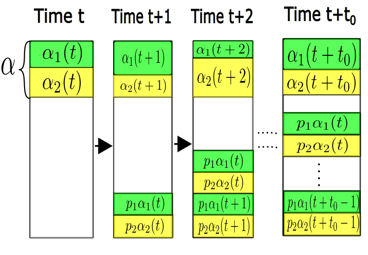
Thereby, at time $t+t_{0}$ where the instantaneous threshold $l_{k}(t+t_{0})\geq t_{0}$, we get a set of proportions
$\{p_{1}\alpha_{1}(t),p_{2}\alpha_{2}(t),\cdots,p_{1}\alpha_{1}(t+t_{0}-1),p_{2}\alpha_{2}(t+t_{0}-1)\}$ that belong to the proportion $1-\alpha$ of users with the lowest Whittle index values, such that $z_{1}^{1}(t+t_{0})=p_{1}\alpha_{1}(t+t_{0}-1)$, $z_{1}^{2}(t+t_{0})=p_{2}\alpha_{2}(t+t_{0}-1)$, $\cdots$, $z^{1}_{t_{0}}(t+t_{0})=p_{1}\alpha_{1}(t)$ and $z^{2}_{t_{0}}(t+t_{0})=p_{2}\alpha_{2}(t)$. Hence, we obtain a $z^{k}_{i}(t+1)$ which is well expressed in function of terms of $\alpha_{k}(\cdot)$ ($k=1,2$) for $i\in[1,t_{0}]$, $k=1,2$.

Based on this remark above, we need to find at time $t+t_{0}$, a set of the form $\{z^{k}_{i}(t+t_{0}):w_{k}(i)\leq w_{m}(n)\}$ for a given class $m$ and state $n$, such all the elements of this set are well expressed in function of $\alpha_{k}(\cdot)$. We show in the sequel that the highest Whittle index of this set could be $w_{2}(t_{0})$.

Indeed, given that the Whittle index function is increasing with $n$ where $n$ refers to a given age of information state, then for any state in class $2$ with Whittle index less than $w_{2}(t_{0})$, belongs to $[1,t_{0}]$. Moreover, considering the state $q$ in class $1$ such that $w_{1}(q)\leq w_{2}(t_{0})\leq w_{1}(t_{0})$ ($p_{1}>p_{2}$), then $w_{1}(q)\leq w_{1}(t_{0})$, which means that $q\in[1,t_{0}]$. Hence, for any element in $\{z^{k}_{i}(t+t_{0}):w_{k}(i)\leq w_{2}(t_{0})\}$, can be expressed in function of terms of $\alpha_{k}(\cdot)$ ($k=1,2$). Accordingly, $\{z^{k}_{i}(t+t_{0}):w_{k}(i)\leq w_{2}(t_{0})\}$ equals to the set $\{p_{2}\alpha_{2}(t),\cdots,p_{2}\alpha_{2}(t+t_{0}-1),p_{1}\alpha_{1}(t+t_{0}-l(t+t_{0})),\cdots,p_{1}\alpha_{1}(t+t_{0}-1)\}$, where $l(t+t_{0})$ is the greatest state $q$ in class $1$ such that $w_{1}(q)\leq w_{2}(t_{0})$. We note that $l(t+t_{0})\leq t_{0}$ because $w_{2}(l(t+t_{0}))\leq w_{1}(l(t+t_{0}))\leq w_{2}(t_{0})$.
Therefore, in that regards, for a fixed $t$, we associate for each $t_{0}$ the corresponding sum $\sum_{j=1}^{l(t+t_{0})}z_{j}^{1}(t+t_{0})+\sum_{j=1}^{t_{0}}z_{j}^{2}(t+t_{0})=\sum_{j=1}^{l(t+t_{0})}p_{1}\alpha_{1}(t+t_{0}-j)+\sum_{j=1}^{t_{0}}p_{2}\alpha_{2}(t+t_{0}-j)$. To that extent, we define in the following the time $t_{0}$ when this aforementioned sum exceeds $1-\alpha$.

References

- [1] S. Kaul, R. Yates, and M. Gruteser, “Real-time status: How often should one update?” in 2012 Proceedings IEEE INFOCOM, March 2012, pp. 2731–2735.
- [2] B. Buyukates and S. Ulukus, “Timely distributed computation with stragglers. october 2019,” Available on.
- [3] S. Farazi, A. G. Klein, J. A. McNeill, and D. R. Brown, “On the age of information in multi-source multi-hop wireless status update networks,” in 2018 IEEE 19th International Workshop on Signal Processing Advances in Wireless Communications (SPAWC). IEEE, 2018, pp. 1–5.
- [4] A. Maatouk, M. Assaad, and A. Ephremides, “The age of updates in a simple relay network,” in 2018 IEEE Information Theory Workshop (ITW). IEEE, 2018, pp. 1–5.
- [5] P. Zou, O. Ozel, and S. Subramaniam, “Waiting before serving: A companion to packet management in status update systems,” IEEE Transactions on Information Theory, 2019.
- [6] Y. Sun, E. Uysal-Biyikoglu, R. D. Yates, C. E. Koksal, and N. B. Shroff, “Update or wait: How to keep your data fresh,” IEEE Transactions on Information Theory, vol. 63, no. 11, pp. 7492–7508, 2017.
- [7] R. Talak, S. Karaman, and E. Modiano, “Minimizing age-of-information in multi-hop wireless networks,” in 2017 55th Annual Allerton Conference on Communication, Control, and Computing (Allerton). IEEE, 2017, pp. 486–493.
- [8] A. M. Bedewy, Y. Sun, and N. B. Shroff, “Age-optimal information updates in multihop networks,” in 2017 IEEE International Symposium on Information Theory (ISIT). IEEE, 2017, pp. 576–580.
- [9] A. Kosta, N. Pappas, A. Ephremides, and V. Angelakis, “Age of information performance of multiaccess strategies with packet management,” Journal of Communications and Networks, vol. 21, no. 3, pp. 244–255, 2019.
- [10] Y. Sun, E. Uysal-Biyikoglu, and S. Kompella, “Age-optimal updates of multiple information flows,” in IEEE INFOCOM 2018-IEEE Conference on Computer Communications Workshops (INFOCOM WKSHPS). IEEE, 2018, pp. 136–141.
- [11] E. T. Ceran, D. Gündüz, and A. György, “Average age of information with hybrid arq under a resource constraint,” IEEE Transactions on Wireless Communications, vol. 18, no. 3, pp. 1900–1913, 2019.
- [12] A. Maatouk, M. Assaad, and A. Ephremides, “On the age of information in a csma environment,” IEEE/ACM Transactions on Networking, vol. 28, no. 2, pp. 818–831, 2020.
- [13] Z. Jiang, B. Krishnamachari, X. Zheng, S. Zhou, and Z. Niu, “Timely status update in massive iot systems: Decentralized scheduling for wireless uplinks,” arXiv preprint arXiv:1801.03975, 2018.
- [14] R. Talak, S. Karaman, and E. Modiano, “Distributed scheduling algorithms for optimizing information freshness in wireless networks,” in 2018 IEEE 19th International Workshop on Signal Processing Advances in Wireless Communications (SPAWC). IEEE, 2018, pp. 1–5.
- [15] I. Kadota, A. Sinha, E. Uysal-Biyikoglu, R. Singh, and E. Modiano, “Scheduling policies for minimizing age of information in broadcast wireless networks,” IEEE/ACM Transactions on Networking, vol. 26, no. 6, pp. 2637–2650, 2018.
- [16] P. Ansell, K. D. Glazebrook, J. Niño-Mora, and M. O’Keeffe, “Whittle’s index policy for a multi-class queueing system with convex holding costs,” Mathematical Methods of Operations Research, vol. 57, no. 1, pp. 21–39, 2003.
- [17] S. Kriouile, M. Larranaga, and M. Assaad, “Asymptotically optimal delay-aware scheduling in wireless networks,” arXiv preprint arXiv:1807.00352, 2018.
- [18] ——, “Whittle index policy for multichannel scheduling in queueing systems,” in 2019 IEEE International Symposium on Information Theory (ISIT). IEEE, 2019, pp. 2524–2528.
- [19] M. Larrañaga, M. Assaad, A. Destounis, and G. S. Paschos, “Asymptotically optimal pilot allocation over markovian fading channels,” IEEE Transactions on Information Theory, 2017.
- [20] K. Liu and Q. Zhao, “Indexability of restless bandit problems and optimality of whittle index for dynamic multichannel access,” IEEE Transactions on Information Theory, vol. 56, no. 11, pp. 5547–5567, 2010.
- [21] A. Maatouk, S. Kriouile, M. Assaad, and A. Ephremides, “On the optimality of the whittle’s index policy for minimizing the age of information,” arXiv preprint arXiv:2001.03096, 2020.
- [22] W. Ouyang, A. Eryilmaz, and N. B. Shroff, “Downlink scheduling over markovian fading channels,” IEEE/ACM Transactions on Networking, vol. 24, no. 3, pp. 1801–1812, 2015.
- [23] K. P. Papadaki and W. B. Powell, “Exploiting structure in adaptive dynamic programming algorithms for a stochastic batch service problem,” European Journal of Operational Research, vol. 142, no. 1, pp. 108–127, 2002.
- [24] R. R. Weber and G. Weiss, “On an index policy for restless bandits,” Journal of Applied Probability, vol. 27, no. 3, pp. 637–648, 1990.
- [25] P. Whittle, “Restless bandits: Activity allocation in a changing world,” Journal of applied probability, vol. 25, no. A, pp. 287–298, 1988.
- [26] C. H. Papadimitriou and J. N. Tsitsiklis, “The complexity of optimal queuing network control,” Mathematics of Operations Research, vol. 24, no. 2, pp. 293–305, 1999.
- [27] T. G. Kurtz, “Strong approximation theorems for density dependent markov chains,” Stochastic Processes and their Applications, vol. 6, no. 3, pp. 223–240, 1978.
Appendix A Proof of Lemma 1
We can formulate the fluid limit equation (18) as follows:
At time , applying Whittle index policy, in average exactly a proportion of of users will be at state one since refers to the proportion of users in class that are scheduled. Accordingly, . While for , the users’ proportion is not scheduled. Therefore at time , since prescribing idle action to a given user implies that its state will be increased by , the proportion at state in class will be at state . Thus, ..
Appendix B Proof of Lemma 2
First of all, we provide an useful lemma.
Lemma 5.
We have for all integer and for :
Proof.
renewcommand∎ The result can be obtained directly by replacing by its expression. ∎
In order to prove the present lemma, we proceed in two steps:
- •
We prove first by contradiction that there exists a given time such that .
We prove that if , then for all .
- 1.
For the first point, we suppose that for all , we have that . Consequently, we get that , and . This means that, the proportion of all users in class is equal to . However, the users’ proportion of class is . That is, there exists a given time such .
- 2.
Before addressing the second point, we recall that refers to the scheduled users’ proportion in the class . Thereby, contains all users with the highest Whittle index values among all users in class . To that extent, at time , the Whittle index of is greater than the Whittle index of the users’ proportion that we denote by . We let be the set of pair (state,class) at time in the users’ proportion . Denoting by the smallest state of , and a given state and class respectively such that belongs to at time , then . Under the Whittle index policy, at time , the states of a users’ proportion that equals to among the users’ proportion , will be increased by one in comparison with the time slot , as well as the users’ proportion . Accordingly, the smallest state of the proportion , is . is shifted of one with respect to , i.e., . We compare with the Whittle index of in class such that . In that direction, we let , and we distinguish between two cases:
: Leveraging the fact that , then . That implies that since is increasing. Hence . As consequence,
: Again we distinguish between two case:
- –
If , then .
Therefore, we obtain our desired result for the first case. - –
If :
We have that:Applying Lemma 5, we obtain: . Given that , therefore replacing by their expressions we get:
As , then:
Hence:
Therefore, . Hence, knowing that we end up with our desired result for this case, i.e. .
Thus, we have proved that at time , all the users’ proportions in whose sum is equal to have a Whittle index less than that of defined in the beginning of this proof. That means that there exists at least a users’ proportion that equals to with Whittle index values less than those of the states of the users’ proportion . Then surely, the users’ proportion that is different from belongs to the users’ proportion with the highest Whittle index values. This implies that surely at time , there will be at least one queue in class 1 belonging to with the highest Whittle index values. Therefore, we have that . This result can be generalized for all . In other words, we have for all , .
Appendix C Proof of Lemma 3
As for all integers , then, if , .
For , we have that . This means that is equal to , which implies that . Moreover, knowing that , then for all , . Hence, we get that , for all .
Therefore, according to the definition 2, satisfies: