跳到论文正文
W Papers独立论文阅读器 arXiv:2102.02472 论文正文 计算阅读时间 · 0%
引用这篇论文根据当前论文元数据生成,正式投稿前建议核对。


License: CC BY 4.0
arXiv:2102.02472v2 [cs.LG] 25 Jun 2021

Transfer Learning in Bandits with Latent Continuity

Hyejin Park21, Seiyun Shin31, Kwang-Sung Jun4, and Jungseul Ok2 Affiliation: 2POSTECH, {parkebbi2, jungseul}@postech.ac.kr Affiliation: 3University of Illinois at Urbana-Champaign, seiyuns2@illinois.edu Affiliation: 4University of Arizona, kjun@cs.arizona.edu
Abstract

Structured stochastic multi-armed bandits provide accelerated regret rates over the standard unstructured bandit problems. Most structured bandits, however, assume the knowledge of the structural parameter such as Lipschitz continuity, which is often not available. To cope with the latent structural parameter, we consider a transfer learning setting in which an agent must learn to transfer the structural information from the prior tasks to the next task, which is inspired by practical problems such as rate adaptation in wireless link. Specifically, we propose a simple but efficient framework to provably and accurately estimate the Lipschitz constant based on previous tasks and fully exploit it for the new task at hand. We analyze the efficiency of the proposed framework in two folds: (i) our regret bound on the new task is close to that of the oracle algorithm with the full knowledge of the Lipschitz constant under mild assumptions; and (ii) the sample complexity of our estimator matches with the information-theoretic fundamental limit. Our analysis reveals a set of useful insights on transfer learning for latent Lipschitz constants such as the fundamental challenge a learner faces. Finally, our numerical evaluations confirm our theoretical findings and show the superiority of the proposed framework compared to baselines.

**footnotetext: Authors contributed equally.

I Introduction

The classical stochastic multi-armed bandit (MAB) [1] of independent KK arms in time-horizon TT has the fundamental limit of regret O⁡(K​log⁡T)O(K\log T) which scales linearly with the number of arms KK and thus not practical when KK is very large. To deal with large number of arms, one may exploit known correlations among the arms via a structural assumption. This idea has resulted in a stream of research activities on bandits under a variety of structural assumptions, e.g., Lipschitz [2], linear [3], convex [4], or unimodal [5]. These studies are meaningful in deriving bandit algorithms whose regret is scale-free, indicating that it does not grow with KK for large enough KK. In case of the Lipschitz continuity structure described by a Lipschitz constant LL [6], for example, one can achieve O⁡(min⁡{K,poly​(L)}​log⁡T)O(\min\{K,\text{poly}(L)\}\log T).

Such a benefit from the continuity structure, however, requires prior knowledge on the Lipschitz constant LL, which is often latent in practice. In this case, it is natural to estimate the latent LL from similar tasks. For example, rate adaptation in wireless link [7, 8] faces a sequence of bandit problems with similar structural properties, while one can find a continuity structure among throughputs of transmission rates. The channel often changes discretely over time, and these changes partition a sequence of tasks as in our learning scenarios. This motivates us to study a transfer learning problem where we aim to learn the latent Lipschitz constant LL from previous tasks and use it for the next task.

In order to build provably sample-efficient algorithms for the transfer bandit problem, we first investigate the risks of using wrong estimation of Lipschitz constant LL in two main failure scenarios (Section II-C). Overestimating LL leads to an unnecessary regret, attenuating the benefit from the structure such as scale-free regret. On the other hand, underestimating LL can cause a catastrophic failure of suffering a linear regret. We design an estimator for LL, which balances between the two extremes. We show that using this estimator, one can nearly achieve the minimal regret of the oracle algorithm knowing LL exactly (Section III-B). Furthermore, our estimator is asymptotically optimal in that the sample complexity on previous tasks matches to the one in a fundamental limit analysis. Finally, we conclude with numerical verification of our theoretical findings (Section IV) with exciting future directions.

Related work. In [9], the authors provide a generic approach to construct optimal algorithms when we have the complete knowledge on the structural property, including but not limited to Lipschitz [2], linear [3], convex [4], or unimodal [5]. The structural knowledge, however, is often incomplete in practice as mentioned above. For this issue, in [10], it is shown to be possible to achieve the minimax optimal regret of Θ⁡(LD/(D+2)​T(D+1)/(D+2))\Theta(L^{D/(D+2)}T^{(D+1)/(D+2)}) without any knowledge of the Lipschitz constant for the continuum of arms, where DD is the dimension of the embedding space. The minimax optimality compares the regret upper bound of the algorithm to the worst lower bound of regret. Although such a minimax analysis is inevitable for the continuum of arms, a minimax optimal algorithm can be very far from the instant-dependent optimality particularly in canonical cases. Thus, although achieving both minimax and instance-dependent optimality is an active area of research [11], we focus on the instance-dependent regret bounds.

The pioneering work of [12] has proposed a transfer learning framework where the learner faces a sequence of bandit tasks that are randomly drawn from a distribution over a finite set of problem instances. They propose an algorithm that leverages the robust tensor power method to learn the underlying set of instances while repeatedly solving each task. Their algorithms, however, only consider a finite number of instances, in contrast to our Lipschitz structure which consists of infinitely many instances. While there have been a few follow-up studies for infinite instance sets such as [13, 14], they both consider the simple linear structure and focus on minimax regret rather than instance-dependent regret. To our knowledge, we are the first to study transfer learning in bandits with instance-dependent optimality beyond the simple case of the finite instance set.

II Preliminary

II-A Lipschitz bandit model

Let 𝝁=(μ⁡(1),…,μ⁡(K))\bm{\mu}=(\mu(1),...,\mu(K)) denote a multi-armed bandit instance, where each play of arm i∈[K]:={1,2,…,K}i\in[K]\mathrel{\mathop{\ordinarycolon}}=\{1,2,...,K\} generates a reward drawn i.i.d. from Bernoulli distribution with mean μ⁡(i)∈[0,1]\mu(i)\in[0,1]. Notice that the choice of reward distribution and our analysis can be generalized to those related to exponential family with a single parameter [15, 16], but for ease of exposition, we restrict our attention to Bernoulli rewards. At each round t=1,2,…,t=1,2,..., the decision maker π\pi selects an arm iti_{t}, pulls it, and then receives a reward rtr_{t} drawn from the distribution associated with the arm iti_{t}. Let μ∗:=maxi∈[K]⁡μ⁡(i)\mu_{*}\mathrel{\mathop{\ordinarycolon}}=\max_{i\in[K]}\mu(i) and 𝒦∗(𝝁):={i∈[K]:μ(i)=μ∗}\mathcal{K}_{*}(\bm{\mu})\mathrel{\mathop{\ordinarycolon}}=\{i\in[K]\mathrel{\mathop{\ordinarycolon}}\mu(i)=\mu_{*}\} denote the best mean reward and the set of best arms, respectively. For a given MAB instance 𝝁\bm{\mu}, an algorithm π\pi aims to maximize the expected cumulative rewards over the time horizon TT. This aim is equivalent to minimizing the regret defined as follows:

RTπ​(𝝁):=∑i∈[K](μ∗−μ⁡(i))​𝔼π​[nT​(i)],\displaystyle R^{\pi}_{T}(\bm{\mu})\mathrel{\mathop{\ordinarycolon}}=\sum_{i\in[K]}(\mu_{*}-\mu(i))\mathbb{E}_{\pi}[n_{T}(i)]\;,

where nT​(i)n_{T}(i) is the number of pulling arm ii up to time TT, and the expectation 𝔼π\mathbb{E}_{\pi} is taken w.r.t. the randomness induced by both the rewards and the algorithm π\pi. The regret RTπ​(𝝁)R^{\pi}_{T}(\bm{\mu}) can also be viewed as the expected opportunity cost for selecting sub-optimal arms.

II-B Optimal regret with known LL

We consider the set of mean rewards where the arms are constrained to satisfy Lipschitz condition w.r.t. an embedding of the arms 𝒙=(x⁡(1),…,x⁡(K))∈[0,1]D×K\bm{x}=(x(1),...,x(K))\in[0,1]^{D\times K}, which is commonly referred to as the Lipschitz structure [2]. Specifically, the Lipschitz structure Φ⁡(L)\Phi(L) for a given Lipschitz constant L>0L>0 is defined as follows:

Φ(L):={𝝁∈[0,1]K:|μ(i)−μ(j)|≤Ld(i,j)∀i,j∈[K]},\displaystyle\!\Phi(L)\mathrel{\mathop{\ordinarycolon}}=\left\{\bm{\mu}\!\in\![0,1]^{K}\!\!\mathrel{\mathop{\ordinarycolon}}|\mu(i)\!-\!\mu(j)|\leq Ld(i,j)~\forall i,j\!\in\![K]\right\}\;,

where d⁡(i,j):=‖x⁡(i)−x⁡(j)‖d(i,j)\mathrel{\mathop{\ordinarycolon}}=\|x(i)-x(j)\|. We assume that the learner knows that the instance 𝝁\bm{\mu} conforms to the structure Φ⁡(L)\Phi(L). We say an algorithm π\pi is uniformly good for Φ⁡(L)\Phi(L) if 𝔼π​[nT​(i)]=o⁡(Tρ)\mathbb{E}_{\pi}[n_{T}(i)]=o(T^{\rho}) for all i∉𝒦∗​(𝝁)i\notin\mathcal{K}_{*}(\bm{\mu}), 𝝁∈Φ⁡(L)\bm{\mu}\in\Phi(L), and ρ>0\rho>0. That is, a uniformly good algorithm has ability to adapt to any 𝝁∈Φ⁡(L)\bm{\mu}\in\Phi(L) and enjoys a sublinear regret in TT. Then, uniformly good algorithms have the following fundamental limit:

Theorem 1 (Regret lower bound with known LL [2]).

Let π\pi be a uniformly good algorithm for Φ⁡(L)\Phi(L). For any 𝛍∈Φ⁡(L)\bm{\mu}\in\Phi(L),

lim infT→∞RTπ​(𝝁)log⁡T≥C⁡(𝝁,L),\liminf_{T\to\infty}\frac{R^{\pi}_{T}(\bm{\mu})}{\log T}\geq C(\bm{\mu},L)\;, (1)

where C⁡(𝛍,L)C(\bm{\mu},L) is the optimal value of the following linear programming (LP):

min𝜼≽0\displaystyle\underset{\bm{\eta}\succcurlyeq 0}{\textnormal{min}} ∑i∉𝒦∗​(𝝁)(μ∗−μ⁡(i))​η​(i)\displaystyle~~\sum_{i\notin\mathcal{K}_{*}(\bm{\mu})}\!\!\big(\mu_{*}-\mu(i)\big)\eta(i) (2a)
s.t. ∑i∉𝒦∗​(𝝁)KL(μ(i)∥νj(i;𝝁,L))η(i)≥1,∀j∉𝒦∗(𝝁).\displaystyle\!\sum_{i\notin\mathcal{K}_{*}(\bm{\mu})}\!\!\!\textnormal{KL}(\mu(i)\|\nu^{j}(i;\bm{\mu},L))\eta(i)\geq 1,\forall j\notin\mathcal{K}_{*}(\bm{\mu}). (2b)

Here νj​(i,𝛍,L):=max⁡{μ⁡(i),μ∗−L​d​(i,j)}\nu^{j}(i;\bm{\mu},L)\mathrel{\mathop{\ordinarycolon}}=\max\{\mu(i),\mu_{*}-Ld(i,j)\} for all i,j∈[K]i,j\in[K], and KL(μ∥ν)\textnormal{KL}(\mu\|\nu) is the Kullback-Leibler divergence between Bernoulli distributions with mean μ\mu and ν\nu, i.e., KL(μ∥ν):=μlog(μ/ν)+(1−μ)log((1−μ)/(1−ν))\textnormal{KL}({\mu}\|{\nu})\mathrel{\mathop{\ordinarycolon}}=\mu\log\left(\mu/\nu\right)+(1-\mu)\log((1-\mu)/(1-\nu)).

Optimal algorithms for known LL: There exist a number of algorithms that provably achieve the fundamental limit in Theorem 1 such as [2, 9, 6]. Briefly, at each iteration tt, the algorithm finds a solution of LP in (2), denoted by 𝜼⁡(𝝁^𝒕,L)\bm{\eta}(\bm{\hat{\mu}_{t}},L), based on estimated parameter 𝝁^t\bm{\hat{\mu}}_{t} and tracks the solution in a suggestion on minimal exploration so that η⁡(i,𝝁^𝒕,L)≤nt​(i)log⁡t{\eta}(i;\bm{\hat{\mu}_{t}},L)\leq\frac{n_{t}(i)}{\log t} for each suboptimal arm ii. We use a simplified version of algorithm proposed in [6], denoted by π⁡(L)\pi(L), which is originally designed for structured Markov decision process. Due to the space limit, we postpone the detailed algorithm to the full version. For any 𝝁∈Φ⁡(L)\bm{\mu}\in\Phi(L), the algorithm π⁡(L)\pi(L) enjoys the following regret upper bound.

Theorem 2 (Regret upper bound with known LL [2]).

Consider 𝛍∈Φ⁡(L)\bm{\mu}\in\Phi(L) such that for each i∉𝒦∗​(𝛍)i\notin\mathcal{K}_{*}(\bm{\mu}), the LP solution η⁡(i,𝛍,L)\eta(i;\bm{\mu},L) is unique and continuous at 𝛍\bm{\mu}. Then, for any given λ>0\lambda>0, algorithm π=π⁡(L)\pi=\pi(L) has

lim supT→∞RTπ​(𝝁)log⁡T≤(1+λ)​C​(𝝁,L).\limsup_{T\to\infty}\frac{R^{\pi}_{T}(\bm{\mu})}{\log T}\leq(1+\lambda)C(\bm{\mu},L)\;. (3)

Theorem 2 implies that when using exact value of LL, we can asymptotically achieve the regret lower bound in Theorem 1. It is worth noting that exploiting the exact Lipschitz structure provides a drastic reduction in regret:

Property 1.

Let Δ𝛍:=mini∉𝒦∗​(𝛍)⁡μ∗−μ⁡(i)\Delta_{\bm{\mu}}\mathrel{\mathop{\ordinarycolon}}=\min_{i\notin\mathcal{K}_{*}(\bm{\mu})}\mu_{*}-\mu(i) denote the smallest suboptimality gap. Then, for L>0L>0 and 𝛍∈Φ⁡(L)\bm{\mu}\in\Phi(L),

C⁡(𝝁,L)≤8Δ𝝁2​min⁡{K,(8​L​DΔ𝝁+1)D}.\displaystyle C(\bm{\mu},L)\leq\frac{8}{\Delta^{2}_{\bm{\mu}}}\min\left\{K,\left(\frac{8L\sqrt{D}}{\Delta_{\bm{\mu}}}+1\right)^{D}\right\}\;. (4)

Given a fixed Δ𝝁\Delta_{\bm{\mu}} and DD, the fundamental limit of regret C⁡(𝝁,L)C(\bm{\mu},L) is scale-free, meaning that it does not scale with the number of arms KK. In particular, this is a dramatic advantage over no continuity structure, i.e., L=∞L=\infty, whose optimal regret does scale with KK.

(a) Bandit parameter 𝝁\bm{\mu} and embedding 𝒙\bm{x} with L=200L=200
Refer to caption
(b) Regret over time
Fig. 1: Comparison among π⁡(∞)\pi(\infty), π⁡(200)\pi(200), π⁡(0.1)\pi(0.1) and π⁡(L^t)\pi(\hat{L}_{t}) for given 𝝁\bm{\mu} and 𝒙\bm{x} shown in Figure 1(a).

II-C Impact of incorrect estimation of LL

In the context of latent Lipschitz constant LL, one needs to estimate LL from observed samples, which can be quite inaccurate. We study the impact of using an incorrect estimator L′L^{\prime} in the following two cases: (i) L′>LL^{\prime}>L; and (ii) L′<LL^{\prime}<L.

(i) L′>LL^{\prime}>L: In this case, the regret of algorithm π⁡(L′)\pi(L^{\prime}) is provably bounded from above C⁡(𝝁,L′)C(\bm{\mu},L^{\prime}), and thus causes a larger regret. This follows from the fact that for any L′≥LL^{\prime}\geq L, Φ⁡(L)⊂Φ⁡(L′)\Phi(L)\subset\Phi(L^{\prime}), so we have C⁡(𝝁,L)≤C⁡(𝝁,L′)C(\bm{\mu},L)\leq C(\bm{\mu},L^{\prime}), ∀𝝁∈Φ⁡(L)\forall\bm{\mu}\in\Phi(L). The regret rate of algorithm π⁡(L′)\pi(L^{\prime}) can be degenerated into that of the unstructured case due to the conservative choice of L′L^{\prime}. Then, the regret must scale with KK as discussed above, which is problematic for larger KK’s.

(ii) L′<LL^{\prime}<L: In this case, L′L^{\prime} is underestimated, which implies that 𝝁∈Φ⁡(L)∖Φ⁡(L′)≠∅\bm{\mu}\in\Phi(L)\setminus\Phi(L^{\prime})\neq\emptyset. Therefore, the regret bound stated above does not hold anymore. The algorithm π⁡(L′)\pi(L^{\prime}) may suffer a linear regret because once the algorithm starts exploiting an incorrect best arm, it may not be able to collect sufficient statistical evidence to correct itself.

We confirm this phenomenon by a numerical simulation in Figure 1, where the mean rewards of 6 arms 𝝁=(0.1,0.0005,0.0005,0.2005,0.0005,0.0005)\bm{\mu}=(0.1,0.0005,0.0005,0.2005,0.0005,0.0005) and their embedding 𝒙=(0,0.995,0.996,0.997,0.998,0.999)\bm{x}=(0,0.995,0.996,0.997,0.998,0.999) are illustrated in Figure 1(a). We set the true Lipschitz constant LL to be 200200 and the second steepest slope to be 0.10.1. For each time step tt, we define the estimator L^t:=maxi≠j∈[K]⁡|μ^t​(i)−μ^t​(j)|d⁡(i,j)\hat{L}_{t}\mathrel{\mathop{\ordinarycolon}}=\max_{i\neq j\in[K]}\frac{|\hat{\mu}_{t}(i)-\hat{\mu}_{t}(j)|}{d(i,j)}. With the time horizon T=50,000T=50,000, Figure 1(b) compare four algorithms: (a)​π​(∞)(a)\ \pi(\infty); (b)​π​(L^t)(b)\ \pi(\hat{L}_{t}); (c)​π​(200)(c)\ \pi(200); and (d)​π​(0.1)(d)\ \pi(0.1). We remark that π⁡(L^t)\pi(\hat{L}_{t}) updates the estimator after each time step. We observe that the most conservative choice of L=∞L=\infty and the exact choice of L=200L=200 show similar logarithmic regrets. On the other hand, the aggressive choice of L=0.1L=0.1 suffers from an almost linear regret due to the mismatch between the true structure and its belief. The last method π⁡(L^t)\pi(\hat{L}_{t}) also shows an almost linear regret and even worse regret than π⁡(0.1)\pi(0.1), despite keeping to update its estimator for LL. This is because the Lipschitz constant is underestimated by undersampling the hidden true best arm 44 (i.e., x=0.997x=0.997). This underestimated L^t\hat{L}_{t} reinforces the algorithm to reduce the exploration rate on the true best arm, thus losing the opportunity to correct L^t\hat{L}_{t}.

To summarize, our simulation shows that simultaneously learning structure and minimizing regret in π⁡(L^t)\pi(\hat{L}_{t}) in transfer learning setting is highly nontrivial and cannot be done via naive methods.

III Main Results

III-A Transfer learning model
Refer to caption
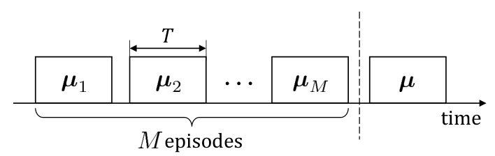
Fig. 2: Transfer learning from previous MM episodes.

Hereafter, we assume that the Lipschitz constant L>0L>0 is latent, although we know the embedding 𝒙\bm{x} in advance, i.e., the relative similarity (d⁡(i,j))i,j∈[K](d(i,j))_{i,j\in[K]} among the arms. To learn latent LL, we consider a scenario of transfer learning illustrated in Figure 2 where one aims to transfer the knowledge on LL extracted from MM past episodes with the mean rewards (𝝁m)m∈[M](\bm{\mu}_{m})_{m\in[M]} satisfying 𝝁m∈Φ⁡(L)\bm{\mu}_{m}\in\Phi(L) to a new episode (M+1)(M+1) with mean rewards 𝝁∈Φ⁡(L)\bm{\mu}\in\Phi(L). For simplicity, we assume that each episode has the same length TT. Let Lm:=maxi≠j∈[K]⁡|μm​(i)−μm​(j)|‖x⁡(i)−x⁡(j)‖L_{m}\mathrel{\mathop{\ordinarycolon}}=\max_{i\neq j\in[K]}\frac{|\mu_{m}(i)-\mu_{m}(j)|}{\|x(i)-x(j)\|} be the tightest Lipschitz constant of episode mm. Note that maxm∈[M]⁡Lm≤L\max_{m\in[M]}L_{m}\leq L. We make the following assumption on LmL_{m}’s:

Assumption 1 (Learnability).

At least α\alpha-portion of the previous MM episodes have their LmL_{m} close to LL with certain margin εα>0\varepsilon_{\alpha}>0. Formally, there exist α>0\alpha>0 and εα>0\varepsilon_{\alpha}>0 such that

|{m∈[M]:Lm≥L−εα}|≥αM.\displaystyle|\{m\in[M]\mathrel{\mathop{\ordinarycolon}}L_{m}\geq L-\varepsilon_{\alpha}\}|\geq\alpha M\;.

The parameters α\alpha and εα\varepsilon_{\alpha} in Assumption 1 quantify the difficulty of estimating LL tightly, where larger α\alpha and smaller εα\varepsilon_{\alpha} imply sharper concentration of LmL_{m}’s around LL and thus easier setting. Recalling that smaller LL implies smaller regret, we aim to estimate the smallest possible LL. Notice that L=maxm∈[M]⁡LmL=\max_{m\in[M]}L_{m} can be easily manipulated with any large LmL_{m}. We can assume a prior distribution of bandit parameter over structure Φ⁡(L)\Phi(L) instead of Assumption 1, but it is somewhat impractical to know this. Thus, through the assumption on tail distribution of LmL_{m}’s which allows a robust estimation of LL, it is possible to securely recover the Lipschitz constant. In addition, our analysis under Assumption 1 can be easily applied to the case assuming prior distribution of bandit parameter. The difficulty of estimating LL also depends on the sampling scheme in the prior tasks. Hence, we make the following assumption:

Assumption 2 (Minimal exploration).

For each episode mm, every arm i∈[K]i\in[K] is pulled at least τ>0\tau>0.

In Assumption 2, a small value of τ\tau implies a high risk of having insufficient samples for estimation of LL.

III-B Extracting Lipschitz constant

To analyze with latent LL, we take a two-folded approach. First, we estimate LL from extracting structural information in previous MM episodes. We then run π⁡(L^β)\pi(\hat{L}_{\beta}), where L^β\hat{L}_{\beta} is the estimate LL. Let 𝝁^m\hat{\bm{\mu}}_{m} be the estimated mean rewards and L^m:=maxi≠j∈[K]⁡|μ^m​(i)−μ^m​(j)|‖x⁡(i)−x⁡(j)‖{\hat{L}_{m}}\mathrel{\mathop{\ordinarycolon}}=\max_{i\neq j\in[K]}\frac{|\hat{\mu}_{m}(i)-\hat{\mu}_{m}(j)|}{\|x(i)-x(j)\|} be the estimated Lipschitz constant in episode mm. For an efficient estimate of LL, we introduce two hyperparameters β∈(0,α)\beta\in(0,\alpha) and εβ>εα\varepsilon_{\beta}>\varepsilon_{\alpha}. We set our estimator as an upper confidence bound on LL:

L^β:=ℓβ+εβ.\displaystyle\hat{L}_{\beta}\mathrel{\mathop{\ordinarycolon}}=\ell_{\beta}+\varepsilon_{\beta}. (5)

Here ℓβ:=⌈β​M⌉​-​maxm∈[M]⁡L^m\ell_{\beta}\mathrel{\mathop{\ordinarycolon}}=\mathop{\lceil\beta M\rceil{\text{-\hskip-0.59998pt}}\max}_{m\in[M]}~\hat{L}_{m}, where k​-​max\mathop{k{\text{-\hskip-0.59998pt}}\max} denotes the operator taking the kk-th largest element. Note that the margin εβ\varepsilon_{\beta} is imposed to reduce the risk of underestimating LL since structured bandit algorithms with the underestimated Lipschitz constant can induce almost linear regret as shown in Section II-C. By running π⁡(L^β)\pi(\hat{L}_{\beta}), we get the following performance guarantee:

Theorem 3.

Suppose Assumptions 1 and 2 hold for α>0\alpha>0 and εα>0\varepsilon_{\alpha}>0. Let β∈(0,α)\beta\in(0,\alpha) and τ≥4Δ𝐱2​(εβ−εα)2​(ln⁡(2​K)+1min⁡{β,α−β})\tau\geq{\frac{4}{\Delta^{2}_{{\bm{x}}}(\varepsilon_{\beta}-\varepsilon_{\alpha})^{2}}}\left(\ln(2K)+\frac{1}{\min\{\beta,\alpha-\beta\}}\right). If M≥2​Z​ln⁡(2​Z​T)M\geq 2Z\ln(2ZT) with Z=1min⁡{β,α−β}​ln⁡(2​K)Z={\frac{1}{\min\mathinner{\left\{\beta,\alpha-\beta\right\}}\ln(2K)}}, for any 𝛍∈Φ⁡(L){{\bm{\mu}}}\in\Phi(L), algorithm π⁡(L^β)\pi(\hat{L}_{\beta}) with λ>0\lambda>0 has

lim supT→∞RTπ​(𝝁)log⁡T≤(1+λ)​C​(𝝁,L+2​εβ−εα).\displaystyle\limsup_{T\to\infty}\frac{R^{\pi}_{T}(\bm{\mu})}{\log T}\leq(1+\lambda)\ C\!\left(\bm{\mu},L+2\varepsilon_{\beta}-\varepsilon_{\alpha}\right).
Proof.

See Section III-D. ∎

The upper bound of C⁡(𝝁,L′)C(\bm{\mu},L^{\prime}) in (4) is continuous L′L^{\prime} for L′≥LL^{\prime}\geq L and 𝝁∈Φ⁡(L)\bm{\mu}\in\Phi(L). Besides, under mild additional assumptions, we also have a continuity of C⁡(𝝁,L′)C(\bm{\mu},L^{\prime}) in L′L^{\prime} for L′∈[L,L+ε)L^{\prime}\in[L,L+\varepsilon) and 𝝁∈Φ⁡(L)\bm{\mu}\in\Phi(L). We provide a formal description of continuity of C⁡(𝝁,L)C(\bm{\mu},L) in LL, implying a near optimality of the regret upper bound of π⁡(Lβ)\pi(L_{\beta}).

Theorem 4.

For given bandit structure Φ⁡(L′)\Phi(L^{\prime}) with fixed 𝛍\bm{\mu} and 𝐱\bm{x}, the optimal value of (2a)–(2b), L′→C⁡(𝛍,L′)L^{\prime}\rightarrow C(\bm{\mu},L^{\prime}) is continuous in [L,L+δ)[L,L+\delta), provided that the optimal arm x∗​(𝛍)x^{*}(\bm{\mu}), the solution to problem (2a)–(2b) in Theorem 1, are unique and δ\delta satisfies

0≤δ<mini,j∈[K]⁡{μ∗−μ⁡(i)‖x⁡(i)−x⁡(j)‖−L},\displaystyle 0\leq\delta<\min_{i,j\in[K]}\left\{\frac{\mu_{*}-\mu(i)}{\|x(i)-x(j)\|}-L\right\}\;, (6)

such that μ⁡(i)>D​K​δ\mu(i)>\sqrt{DK}\delta and νj​(i,𝛍,L)<1−D​K​δ\nu^{j}(i;\bm{\mu},L)<1-\sqrt{DK}\delta for all i,j∈[K]i,j\in[K].

Hence, Theorem 3 implies that when τ\tau and MM are sufficiently large, i.e., we have rich experiences with prior tasks, the algorithm π⁡(L^β)\pi(\hat{L}_{\beta}) closely achieves the fundamental limit of oracle performance knowing LL in advance. One can interpret τ​M\tau M as the sample complexity for some probably approximately correct (PAC) learning of LL. The sample complexity required in Theorem 3 is

τ​M=Ω⁡(1Δ𝒙2​(εβ−εα)2​α​log⁡T),\displaystyle\tau M=\Omega\left(\frac{1}{{\Delta_{{\bm{x}}}^{2}(\varepsilon_{\beta}-\varepsilon_{\alpha})^{2}}\alpha}\log T\right)\;, (7)

which matches with the information-theoretic lower bound for the PAC learning obtained in Section III-D.

Remark 1 (Hyperparameter choice for L^β\hat{L}_{\beta}).

Theorem 3 includes an intrinsic trade-off for the choice of β\beta, which appears in the requirement of M≥Θ~​(max⁡{1β,1α−β})M\geq\tilde{\Theta}(\max\{{\frac{1}{\beta}},{\frac{1}{\alpha-\beta}}\}). Here Θ~\tilde{\Theta} hides logarithmic factors. Notice that when β\beta is too small (choosing near the top of {L^m}\{\hat{L}_{m}\}), the estimate L^β\hat{L}_{\beta} can be too large and overshoot, whereas when β\beta is too large, the estimate falls below LL, incurring linear regret.

Our theorem also suggests that when a valid (α,εα)(\alpha,\varepsilon_{\alpha}) is available, one should set εβ≈2​εα\varepsilon_{\beta}\approx 2\varepsilon_{\alpha} and β≈α/2\beta\approx\alpha/2. It turns out that the algorithm is then guaranteed to use L^β\hat{L}_{\beta} that is at most 3​εα3\varepsilon_{\alpha} away from LL. When the knowledge on (α,εα)(\alpha,\varepsilon_{\alpha}) is not available, one can see that εβ\varepsilon_{\beta} should be greater than 1/M1/M. This is due to the fact that if we set β=1/M\beta=1/M, then assuming all other variables are fixed, the requirement on MM becomes M=Ω⁡(M​ln⁡(M))M=\Omega(M\ln(M)), which clearly cannot be satisfied for large enough MM. In other words, there is no guarantee that transfer learning will happen with our estimator L^β\hat{L}_{\beta}. This motivates us to adopt a quantile ℓβ\ell_{\beta} to compute L^β\hat{L}_{\beta}, rather than simply setting the estimate as the maximum of LmL_{m}’s.

III-C Lower bound of sample complexity τ​M\tau M

We study a fundamental limit of sample complexity in estimating LL from MM prior tasks. Let τm\tau_{m} denote the number of playing the most under-sampled arm in episode mm. Then, Assumption 2 can be written equivalently as minm∈[M]⁡τm≥τ\min_{m\in[M]}\tau_{m}\geq\tau. For given α>0,εα>0,τ>0\alpha>0,\varepsilon_{\alpha}>0,\tau>0, and ε>εα\varepsilon>\varepsilon_{\alpha}, we say an estimator L^\hat{L} is uniformly good for (α,εα,τ,ε)(\alpha,\varepsilon_{\alpha},\tau,\varepsilon) if for any LL, (𝝁m)m∈[M](\bm{\mu}_{m})_{m\in[M]}, and (τm)m∈[M](\tau_{m})_{m\in[M]} such that 𝝁m∈Φ⁡(L)\bm{\mu}_{m}\in\Phi(L) for each m∈[M]m\in[M] satisfy Assumptions 1 and 2, then

ℙ[L^>L+ε]+ℙ[L^<L]≤o(log⁡TT).\displaystyle\mathbb{P}[\hat{L}>L+\varepsilon]+\mathbb{P}[\hat{L}<L]\leq o\left(\frac{\log T}{T}\right)\;. (8)

The concentration in (8) is a minimal condition to conclude the desired regret upper bound in Theorem 3.

Theorem 5.

Suppose that an estimator L^\hat{L} is uniformly good for α>0,εα>0,τ>0\alpha>0,\varepsilon_{\alpha}>0,\tau>0, and ε>εα\varepsilon>\varepsilon_{\alpha}. Then, we must have

Δ𝒙2​(ε−εα)2​α​τ​M=Ω⁡(log⁡T).\displaystyle{\Delta_{{\bm{x}}}^{2}(\varepsilon-\varepsilon_{\alpha})^{2}}\alpha\tau M=\Omega(\log T)\;. (9)

Note that when we set ε=2​εβ−εα\varepsilon=2\varepsilon_{\beta}-\varepsilon_{\alpha}, the concentration of L^\hat{L} in (8) becomes the one that we need to conclude the regret bound of π⁡(L^)\pi(\hat{L}) in Theorem 3. Hence, Theorem 5 provides a lower bound on τ​M\tau M to obtain the desired concentration of L^\hat{L} as (7) which asymptotically matches with the lower bound on τ​M\tau M in Theorem 2 with β=c​α\beta=c\alpha for any positive constant c<1c<1 since the choice of β\beta implies min⁡{β,α−β}=min⁡{c​α,(1−c)​α}\min\{\beta,\alpha-\beta\}=\min\{c\alpha,(1-c)\alpha\}.

(a) Five incidences of 𝝁m\bm{\mu}_{m}
(b) Evolution of estimation over episodes
(c) Cumulative regret over episode
Fig. 3: Comparison of various estimators using the past experiences for L=5L=5.

III-D Proof of Theorem 3

Let Δ𝒙:=mini≠j|d⁡(i,j)|>0{\color[rgb]{0,0,0}\Delta_{{\bm{x}}}}\mathrel{\mathop{\ordinarycolon}}=\min_{i\neq j}\|d(i,j)\|>0. The key analysis of Theorem 3 lies in deriving the concentration of L^β\hat{L}_{\beta} to LL:

Lemma 1.

Take Assumptions 1 and 2 with α\alpha and εα\varepsilon_{\alpha}. Let β∈(0,α)\beta\in(0,\alpha) and ε′:=εβ−εα>0{\color[rgb]{0,0,0}\varepsilon^{\prime}}\mathrel{\mathop{\ordinarycolon}}=\varepsilon_{\beta}-\varepsilon_{\alpha}>0. If τ≥4Δ𝐱2​(εβ−εα)2​(ln⁡(2​K)+1min⁡{β,α−β})\tau\geq{\frac{4}{\Delta^{2}_{{\bm{x}}}(\varepsilon_{\beta}-\varepsilon_{\alpha})^{2}}}\left(\ln(2K)+\frac{1}{\min\{\beta,\alpha-\beta\}}\right),

ℙ[L>ℓβ+εβ]+ℙ[ℓβ>L+ε′]≤8​M​exp⁡(−Δ𝒙2​ε′24​min⁡{β,(α−β)}​τ​M).\displaystyle\begin{aligned} &\mathbb{P}[L>\ell_{\beta}+\varepsilon_{\beta}]+\mathbb{P}[\ell_{\beta}>L+\varepsilon^{\prime}]\\ &\leq 8M\exp\left(-\frac{\Delta_{{\bm{x}}}^{2}\varepsilon^{\prime 2}}{4}\min\{\beta,(\alpha-\beta)\}\tau M\right)~.\end{aligned} (10)

We leave the detailed proof of Lemma 1 in the full version. To avoid linear regret, we desire to control ℙ[L>ℓβ+εβ]+ℙ[ℓβ>L+ε′]≤O(1/T)\mathbb{P}[L>\ell_{\beta}+\varepsilon_{\beta}]+\mathbb{P}[\ell_{\beta}>L+\varepsilon^{\prime}]\leq O(1/T). From Lemma 1, we use the assumption on τ\tau to bound the RHS of (10) by 8​M​exp⁡(−ln⁡(2​K)​min​{β,(α−β)}​M)8M\exp(-\ln(2K)\min\{\beta,(\alpha-\beta)\}M). Then, it suffices to control

M​exp⁡(−ln⁡(2​K)​min​{β,α−β}​M)≤1T.\displaystyle M\exp\left(-\ln(2K)\min\{\beta,~\alpha-\beta\}M\right)\leq{\frac{1}{T}}.

This takes the form of M​exp⁡(−Z−1​M)≤1/TM\exp(-Z^{-1}M)\leq 1/T for some ZZ, which can be written as M≥Z​ln⁡(M)+Z​ln⁡(T)M\geq Z\ln(M)+Z\ln(T). One can show that a sufficient condition on MM to satisfy this inequality is M≥2​Z​ln⁡(2​Z​T)M\geq 2Z\ln\mathinner{\left(2ZT\right)} where Z=1min⁡{β,α−β}​ln⁡(2​K)Z={\frac{1}{\min\mathinner{\left\{\beta,\alpha-\beta\right\}}\ln(2K)}}.

Define Δ𝝁:=maxi∈[K]⁡μ∗−μ⁡(i)≤1{\color[rgb]{0,0,0}\Delta_{{{\bm{\mu}}}}}\mathrel{\mathop{\ordinarycolon}}=\max_{i\in[K]}\mu_{*}-\mu(i)\leq 1. Assuming the condition on MM holds true, the following regret decomposition concludes the proof:

RTπ​(𝝁)\displaystyle\!\!\!\!R^{\pi}_{T}(\bm{\mu}) ≤𝔼π​[∑i∈[K](μ∗−μ⁡(i))​nT​(i)∣L+ε′+εβ≥L^β≥L]\displaystyle\leq\mathbb{E}_{\pi}\!\bigg[\sum_{i\in[K]}(\mu_{*}-\mu(i))n_{T}(i)\mid L+\varepsilon^{\prime}+\varepsilon_{\beta}\geq\hat{L}_{\beta}\geq L\bigg]
+Δ𝝁T(ℙ[L>L^β]+ℙ[L^β>L+ε′+εβ])\displaystyle\quad+\Delta_{{{\bm{\mu}}}}T\left(\mathbb{P}[L>\hat{L}_{\beta}]+\mathbb{P}[\hat{L}_{\beta}>L+\varepsilon^{\prime}+\varepsilon_{\beta}]\right) (11)
≤(1+λ)​C​(𝝁,L+ε′+εβ)​log⁡T+o⁡(log⁡T)\displaystyle\leq(1+\lambda)C(\bm{\mu},L+\varepsilon^{\prime}+\varepsilon_{\beta})\log T+o(\log T)
+Δ𝝁T⋅8Mexp(−Δ𝒙2​ε′24min{β,(α−β)}τM)\displaystyle\quad+\Delta_{{{\bm{\mu}}}}T\cdot 8M\exp\left(-\tfrac{\Delta_{{\bm{x}}}^{2}\varepsilon^{\prime 2}}{4}\min\{\beta,(\alpha-\beta)\}\tau M\right)
≤(1+λ)​C​(𝝁,L+ε′+εβ)​log⁡T+o⁡(log⁡T),\displaystyle\leq(1+\lambda)C(\bm{\mu},L+\varepsilon^{\prime}+\varepsilon_{\beta})\log T+o(\log T)\;,

where we use Theorem 2.

IV Numerical Evaluation

Setup. For numerical experiments, we consider Lipschitz structure Φ⁡(5)\Phi(5) bandit setting with 6 arms, embedding 𝒙=[0,0.8,0.85,0.9,0.95,1]\bm{x}=[0,0.8,0.85,0.9,0.95,1] and time horizons T=10,000T=10,000. For each episode m∈[M=400]m\in[M=400], 𝝁m∈Φ⁡(L)\bm{\mu}_{m}\in\Phi(L) is independently generated by the following procedure: starting with μ1∈[0.05,0.95]\mu_{1}\in[0.05,0.95] selected uniformly at random, for i=2,3,…,Ki=2,3,...,K, select μi\mu_{i} uniformly at random from [μi−1−L​d​(i−1,i),μi−1+L​d​(i−1,i)]∩[0.05,0.95][\mu_{i-1}-Ld(i-1,i),\mu_{i-1}+Ld(i-1,i)]\cap[0.05,0.95]. Figures 3(a) shows five 𝝁m\bm{\mu}_{m}’s generated from the generative procedure. For every estimator (stated below), we use the same sequence of L^m\hat{L}_{m}’s generated by π⁡(∞)\pi(\infty) that uses no continuity structures.

Stable estimator L^β\hat{L}_{\beta}. Figure 3(b) illustrates the comparison of accuracy between the four estimators on LL: three L^β\hat{L}_{\beta}’s with (β,εβ)∈{(0.5,0.05)(\beta,\varepsilon_{\beta})\in\{(0.5,0.05), (0.3,0.05)(0.3,0.05), (0.1,0.05)}(0.1,0.05)\} and max⁡(L^m)\max(\hat{L}_{m}) which takes the maximum of L^m\hat{L}_{m}’s estimated previously. As expected, the most conservative estimation of max⁡(L^m)\max(\hat{L}_{m}), which can theoretically explode up to 1/Δ𝒙=201/\Delta_{\bm{x}}=20 in a finite number of episodes, has monotonically increased estimation of LL. In contrast, each of L^β\hat{L}_{\beta}’s stabilizes the estimation of Lipschitz constant LL, once we have sufficient experiences, e.g., M>30M>30. Throughout the comparison of three L^β\hat{L}_{\beta}’s, we can observe that the appropriate value of β\beta can bring benefits of Lipschitz continuity. Specifically the appropriate choice of β=0.3\beta=0.3 leads us to obtain an accurate and stable estimation of LL, yielding the lower regret as shown in Figure 3(c).

Cumulative regret. Figure 3(c) describes the cumulative regret under various estimators. We anticipate that the observations among the neighboring arms 22 to 66 (i.e., x∈[0.8,1]x\in[0.8,1]), which are far from the embedding of arm 11, are easily generalized to each other via Lipschitz continuity. As discussed in our theoretical analysis, we observe that the more accurate estimation of LL leads the greater reduction in regret. It suggests that there can be a significant difference according to β\beta we set, which brings meaningful L^β\hat{L}_{\beta}. In particular, the aggressive choice of β=0.5\beta=0.5 gives a risky estimation L^β≲L\hat{L}_{\beta}\lesssim L; hence imposing a margin εβ\varepsilon_{\beta} may be helpful. Therefore, when we do not have information of structure, it is meaningful to transfer information of Lipschitz constant to prior tasks by selecting the appropriate hyperparameter β\beta and ε\varepsilon. We leave more detailed experimental descriptions in the full version.

V Conclusion

We have investigated the role of transfer learning of the unknown Lipschitz continuity. Our main contribution lies in our novel estimator L^β\hat{L}_{\beta}, its information-theoretic optimality, and regret analysis when using L^β\hat{L}_{\beta} for future tasks, which is shown to be close to using the true unknown Lipschitz constant LL both theoretically and empirically. Our results serve as the first step towards transfer learning in structure bandits with tight instance-dependent regret guarantees, which opens up numerous fascinating research directions. For example, it would be interesting to extend our setup to fully adaptive sequential transfer setting where the target accuracy ε\varepsilon is adjusted automatically as the learner solves more episodes. Another direction is to assume that the embedding 𝒙{{\bm{x}}} is not available where the learner must estimate it on the fly.

VI Acknowledgements

This work was partly supported by Institute of Information & communications Technology Planning & Evaluation (IITP) grant funded by the Korea government (MSIT) (No. 2019-0-01906, Artificial Intelligence Graduate School Program (POSTECH)) and (No. 2021-0-00739, Development of Distributed/Cooperative AI based 5G+ Network Data Analytics Functions and Control Technology).

References

  • [1] H. Robbins, “Some aspects of the sequential design of experiments,” Bulletin of the American Mathematics Society, vol. 58, pp. 527–535, 1952.
  • [2] S. Magureanu, R. Combes, and A. Proutiere, “Lipschitz bandits: Regret lower bounds and optimal algorithms,” in Conference on Learning Theory (COLT), 2014.
  • [3] V. Dani, T. P. Hayes, and S. M. Kakade, “Stochastic linear optimization under bandit feedback,” 2008.
  • [4] A. Agarwal, D. P. Foster, D. J. Hsu, S. M. Kakade, and A. Rakhlin, “Stochastic convex optimization with bandit feedback,” in Advances in Neural Information Processing Systems, 2011, pp. 1035–1043.
  • [5] J. Y. Yu and S. Mannor, “Unimodal bandits,” in International Conference on Machine Learning (ICML), 2011, pp. 41–48.
  • [6] J. Ok, A. Proutiere, and D. Tranos, “Exploration in structured reinforcement learning,” in Advances in Neural Information Processing Systems, 2018, pp. 8874–8882.
  • [7] R. Combes, J. Ok, A. Proutiere, D. Yun, and Y. Yi, “Optimal rate sampling in 802.11 systems: Theory, design, and implementation,” IEEE Transactions on Mobile Computing, vol. 18, no. 5, pp. 1145–1158, 2018.
  • [8] H. Qi, Z. Hu, X. Wen, and Z. Lu, “Rate adaptation with thompson sampling in 802.11 ac wlan,” IEEE Communications Letters, vol. 23, no. 10, pp. 1888–1892, 2019.
  • [9] R. Combes, S. Magureanu, and A. Proutiere, “Minimal exploration in structured stochastic bandits,” in Advances in Neural Information Processing Systems, 2017, pp. 1763–1771.
  • [10] S. Bubeck, G. Stoltz, and J. Y. Yu, “Lipschitz bandits without the lipschitz constant,” in International Conference on Algorithmic Learning Theory. Springer, 2011, pp. 144–158.
  • [11] A. Tirinzoni, A. Lazaric, and M. Restelli, “A Novel Confidence-Based Algorithm for Structured Bandits,” in Proceedings of the International Conference on Artificial Intelligence and Statistics (AISTATS), 2020.
  • [12] M. G. Azar, A. Lazaric, and E. Brunskill, “Sequential transfer in multi-armed bandit with finite set of models,” in Advances in Neural Information Processing Systems, 2013, pp. 2220–2228.
  • [13] M. Soare, A. Lazaric, O. Alsharif, and J. Pineau, “Multi-task linear bandits,” in Advances in Neural Information Processing Systems Workshop, 2014.
  • [14] L. Cella, A. Lazaric, and M. Pontil, “Meta-learning with stochastic linear bandits,” in International Conference on Machine Learning (ICML), 2020.
  • [15] A. Garivier and O. Cappé, “The kl-ucb algorithm for bounded stochastic bandits and beyond,” in Proceedings of the 24th annual conference on learning theory, 2011, pp. 359–376.
  • [16] E. Kaufmann, “On bayesian index policies for sequential resource allocation,” arXiv preprint arXiv:1601.01190, 2016.
  • [17] E. Kaufmann, O. Cappé, and A. Garivier, “On the complexity of best-arm identification in multi-armed bandit models,” The Journal of Machine Learning Research, vol. 17, no. 1, pp. 1–42, 2016.
  • [18] A. B. Tsybakov, Introduction to nonparametric estimation. Springer Science & Business Media, 2008.

Appendix A A Simplified version of Directed Exploration Learning Algorithm [6]

Algorithm 1 π⁡(L)\pi(L)
 for t=1,2,…t=1,2,... do
  if ∃i∈[K]\exists i\in[K] s.t. nt​(i)≤log⁡tlog⁡log⁡tn_{t}(i)\leq\frac{\log{t}}{\log{\log{t}}}​†\dagger then
   {Estimation} Play the most under-sampled arm it∈arg​mini∈[K]⁡nt​(i)i_{t}\in\argmin_{i\in[K]}n_{t}(i)
  else if 𝜻t1+λ∈𝒟⁡(𝝁^t,L)\frac{\bm{\zeta}_{t}}{1+\lambda}\in\mathcal{D}(\hat{\bm{\mu}}_{t},L) then
   {Exploitation} Exploit the most under-sampled current best arm it∈arg​mini∈𝒦∗​(𝝁^t)⁡nt​(i)i_{t}\in\argmin_{i\in\mathcal{K}_{*}(\hat{\bm{\mu}}_{t})}n_{t}(i)
  else
   {Exploration} Compute 𝜼⁡(𝝁^t,L)\bm{\eta}(\bm{\hat{\mu}}_{t},L) and set 𝜼t\bm{\eta}_{t} as follows:
ηt​(i)={min⁡{log⁡t​†,𝜼⁡(i,μ^t,L)},if ​i∈𝒦∗​(𝝁);(1+λ)​𝜼​(i,μ^t,L),otherwise.\displaystyle\eta_{t}(i)=\begin{cases}\min\{\log t\textsuperscript{{\color[rgb]{1,0,0}$\dagger$}},\bm{\eta}(i;\hat{\mu}_{t},L)\},&\text{if }i\in\mathcal{K}_{*}(\bm{\mu});\\ (1+\lambda)\bm{\eta}(i;\hat{\mu}_{t},L),&\text{otherwise.}\end{cases} (12)
   Play the most under-explored arm it∈arg​maxi∈[K]⁡(ηt​(i)​log⁡t−nt​(i))i_{t}\in\argmax_{i\in[K]}\left(\eta_{t}(i)\log{t}-n_{t}(i)\right)
  end if
  Update statistics 𝝁^t+1\hat{\bm{\mu}}_{t+1} based on new reward rtr_{t} corresponding to arm iti_{t}: for each i∈[K]i\in[K], set:
nt+1(i)=nt(i)+𝟙[it=i];andμ^t+1(i)=μ^t(i)+𝟙[it=i](rt−μ^t​(i)nt​(i)+1).\displaystyle n_{t+1}(i)=n_{t}(i)+\one[i_{t}=i];\qquad\text{and}\qquad\hat{\mu}_{t+1}(i)=\hat{\mu}_{t}(i)+\one[i_{t}=i]\left(\frac{r_{t}-\hat{\mu}_{t}(i)}{n_{t}(i)+1}\right).
 end for 

†\dagger Positive constants can be multiplied to these terms for stabilizing the empirical behavior without harming the asymptotic optimality in Theorem 2.

Let 𝜼⁡(𝝁,L)∈ℝ¯+K\bm{\eta}(\bm{\mu},L)\in\bar{\mathbb{R}}^{K}_{+} be a solution of LP (2) where we set η⁡(i,𝝁,L)=∞\eta(i;\bm{\mu},L)=\infty for optimal arm i∈𝒦∗​(𝝁)i\in\mathcal{K}_{*}(\bm{\mu}). Then for the suboptimal arm i∉𝒦∗​(𝝁)i\notin\mathcal{K}_{*}(\bm{\mu}), 𝜼⁡(i,𝝁,L)​log⁡t\bm{\eta}(i;\bm{\mu},L)\log t provides a suggestion on minimal exploration at time tt. This motivates to an algorithm that keeps tracking the estimated LP solution 𝜼⁡(μ^t,L)\bm{\eta}(\hat{\mu}_{t},L) (if we knew LL a priori) where μ^t\hat{\mu}_{t} is the estimation of 𝝁\bm{\mu} at time tt. Indeed, there have been a number of algorithms that use this framework to achieve the asymptotic lower bound in Theorem 1 (if LL is known in advance); e.g., Optimal Sampling for Structured Bandit (OSSB) [9] and Directed Exploration Learning (DEL) [6]. In this paper, for a given LL, we use Algorithm 1, denoted by π⁡(L)\pi(L), that is a simplified version of DEL algorithm [6], which is originally designed for structured Markov decision process. We choose DEL algorithm as it has better empirical behavior than OSSB thanks to the careful handling (such as monotization) for cases where the assumptions for the analysis are broken.

Algorithm 1 consists of three phases: estimation, exploitation, and exploration. The estimation phase ensures that every arm is sampled at least Ω⁡(log⁡t/log⁡log​t)\Omega(\log t/\log\log t). This harms no regret asymptotically as log⁡T/log⁡log⁡T=o⁡(log⁡T)\log T/\log\log T=o(\log T), but it ensures concentrations of the estimates 𝝁^t\hat{\bm{\mu}}_{t} and 𝜼⁡(𝝁^t,L)\bm{\eta}(\hat{\bm{\mu}}_{t},L) to 𝝁\bm{\mu} and 𝜼⁡(𝝁,L)\bm{\eta}({\bm{\mu}},L), respectively. Let 𝜻t∈ℝK\bm{\zeta}_{t}\in\mathbb{R}^{K} be the current rate of exploration at time tt such that ζt​(i):=nt​(i)log⁡t{\zeta}_{t}(i)\mathrel{\mathop{\ordinarycolon}}=\frac{n_{t}(i)}{\log t} for every i∈[K]i\in[K]. The algorithm exploits the current best arm if the current exploration is statistically sufficient to identify the best arm, i.e., 𝜻t1+λ∈𝒟⁡(𝝁,L)\frac{\bm{\zeta}_{t}}{1+\lambda}\in\mathcal{D}(\bm{\mu},L) with some positive margin λ>0\lambda>0. If not, then it explores toward clipped LP solution 𝜼t{\bm{\eta}}_{t} defined as:

ηt​(i):={min⁡{log⁡t,𝜼⁡(i,μ^t,L)},if ​i∈𝒦∗​(𝝁);(1+λ)​𝜼​(i,μ^t,L),otherwise..\displaystyle\eta_{t}(i)\mathrel{\mathop{\ordinarycolon}}=\begin{cases}\min\{\log t,\bm{\eta}(i;\hat{\mu}_{t},L)\},&\text{if }i\in\mathcal{K}_{*}(\bm{\mu});\\ (1+\lambda)\bm{\eta}(i;\hat{\mu}_{t},L),&\text{otherwise.}\end{cases}\;.

Appendix B Proof of Lemma 1

We begin with a concentration analysis on L^m\hat{L}_{m} to LmL_{m}. Note that Assumption 2 guarantees that every arm is played at least τ\tau times in each episode. Hence, using Hoeffding’s inequality, it follows that for every m∈[M]m\in[M],

ℙ[|μm(i)−μ^m(i)|≥ε]≤2exp(−2ε2τ),\displaystyle\mathbb{P}\left[|\mu_{m}(i)-\hat{\mu}_{m}(i)|\geq\varepsilon\right]\leq 2\exp\left(-2\varepsilon^{2}\tau\right)\;, (13)

which implies

ℙ[|Lm−L^m|≥ε]≤ℙ[∃i∈[K]:|μ^m(i)−μm(i)|≥ε​Δ𝒙2]≤2​K​exp⁡(−Δ𝒙2​ε2​τ2).\displaystyle\begin{aligned} &\mathbb{P}\left[|L_{m}-\hat{L}_{m}|\geq\varepsilon\right]\\ &\leq\mathbb{P}\left[\exists i\in[K]\mathrel{\mathop{\ordinarycolon}}|\hat{\mu}_{m}(i)-\mu_{m}(i)|\geq\frac{\varepsilon\Delta_{{\bm{x}}}}{2}\right]\\ &\leq 2K\exp\left(-\frac{\Delta_{{\bm{x}}}^{2}\varepsilon^{2}\tau}{2}\right)~.\end{aligned} (14)

For the following proofs, without loss of generality, we assume that L1≥⋯≥LML_{1}\geq\cdots\geq L_{M} and define ξi=L−Li\xi_{i}=L-L_{i} be the Lipschitz gaps.

Bound of ℙ[L>ℓβ+εβ]\mathbb{P}[L>\ell_{\beta}+\varepsilon_{\beta}]. Let us first show the upper confidence bound derivation. Let [x]+=max⁡{0,x}[x]_{+}=\max\mathinner{\left\{0,x\right\}}. Recall that ξm\xi_{m} is nondecreasing by definition. Let S⁡(i)S(i) be the ii-th smallest element of the set SS. Let mβ:=⌈β​M⌉m_{\beta}\mathrel{\mathop{\ordinarycolon}}=\lceil\beta M\rceil. Define 𝒮:={S⊆[M]:|S|=M−mβ+1}\textbf{$\mathcal{S}$}\mathrel{\mathop{\ordinarycolon}}=\{S\subseteq[M]\mathrel{\mathop{\ordinarycolon}}|S|=M-m_{\beta}+1\}. Then,

ℙ⁡(mβ​-​maxm∈[M]⁡L^m≤L−εβ)\displaystyle\PP\mathinner{\left(\mathop{m_{\beta}{\text{-\hskip-0.59998pt}}\max}_{m\in[M]}\hat{L}_{m}\leq L-\varepsilon_{\beta}\right)} ≤∑S∈𝒮∏i=1M−mβ+1ℙ⁡(L^S⁡(i)≤L−εβ)\displaystyle\leq\sum_{S\in\mathcal{S}}\prod_{i=1}^{M-m_{\beta}+1}\PP(\hat{L}_{S(i)}\leq L-\varepsilon_{\beta})
=∑S∈𝒮∏i=1M−mβ+1ℙ⁡(L^S⁡(i)−LS⁡(i)≤−(εβ−ξS⁡(i)))\displaystyle=\sum_{S\in\mathcal{S}}\prod_{i=1}^{M-m_{\beta}+1}\PP\mathinner{\left(\hat{L}_{S(i)}-L_{S(i)}\leq-(\varepsilon_{\beta}-\xi_{S(i)})\right)}
≤∑S∈𝒮∏i=1M−mβ+11∧2​K​exp⁡(−τ2​Δ𝒙2​[εβ−ξS⁡(i)]+2).\displaystyle\leq\sum_{S\in\mathcal{S}}\prod_{i=1}^{M-m_{\beta}+1}1\wedge 2K\exp(-{\frac{\tau}{2}}\Delta^{2}_{{\bm{x}}}[\varepsilon_{\beta}-\xi_{S(i)}]_{+}^{2})~.

Using S⁡(i)≤mβ+i−1​∀i∈[M−mβ+1]S(i)\leq m_{\beta}+i-1\ \forall i\in[M-m_{\beta}+1], we have ξS⁡(i)≤ξmβ+i−1\xi_{S(i)}\leq\xi_{m_{\beta}+i-1}. Then, the RHS above is bounded by

∑S∈𝒮∏i=1M−mβ+11∧2​K​exp⁡(−τ2​Δ𝒙2​[εβ−ξmβ+i−1]+2)\displaystyle\sum_{S\in\mathcal{S}}\prod_{i=1}^{M-m_{\beta}+1}1\wedge 2K\exp(-{\frac{\tau}{2}}\Delta_{{\bm{x}}}^{2}[\varepsilon_{\beta}-\xi_{m_{\beta}+i-1}]_{+}^{2}) =∑S∈𝒮∏m=mβM1∧2​K​exp⁡(−τ2​Δ𝒙2​[εβ−ξm]+2)\displaystyle=\sum_{S\in\mathcal{S}}\prod_{m=m_{\beta}}^{M}1\wedge 2K\exp(-{\frac{\tau}{2}}\Delta_{{\bm{x}}}^{2}[\varepsilon_{\beta}-\xi_{m}]_{+}^{2})
=(MM−mβ+1)​∏m=mβM1∧2​K​exp⁡(−τ2​Δ𝒙2​[εβ−ξm]+2).\displaystyle=\begin{pmatrix}M\\ M-m_{\beta}+1\end{pmatrix}\prod_{m=m_{\beta}}^{M}1\wedge 2K\exp(-{\frac{\tau}{2}}\Delta_{{\bm{x}}}^{2}[\varepsilon_{\beta}-\xi_{m}]_{+}^{2}).

Note that

∏m=mβM1∧2​K​exp⁡(−τ2​Δ𝒙2​[εβ−ξm]+2)\displaystyle\prod_{m=m_{\beta}}^{M}1\wedge 2K\exp(-{\frac{\tau}{2}}\Delta_{{\bm{x}}}^{2}[\varepsilon_{\beta}-\xi_{m}]_{+}^{2}) ≤mins(1∧2​K​exp⁡(−τ2​Δ𝒙2​[εβ−s]+2))|{m≥mβ:ξm≤s}|\displaystyle\leq\min_{s}\mathinner{\left(1\wedge 2K\exp(-{\frac{\tau}{2}}\Delta_{{\bm{x}}}^{2}[\varepsilon_{\beta}-s]_{+}^{2})\right)}^{|\{m\geq m_{\beta}\mathrel{\mathop{\ordinarycolon}}~\xi_{m}\leq s\}|}
≤(a)(1∧2​K​exp⁡(−τ2​Δ𝒙2​(εβ−εα)2))α​M−mβ+1\displaystyle{\stackrel{{\scriptstyle(a)}}{{\leq}}}\mathinner{\left(1\wedge 2K\exp(-{\frac{\tau}{2}}\Delta_{{\bm{x}}}^{2}(\varepsilon_{\beta}-\varepsilon_{\alpha})^{2})\right)}^{\alpha M-m_{\beta}+1}
≤exp⁡((ln⁡(2​K)−τ2​Δ𝒙2​(εβ−εα)2)⋅(α−β)​M),\displaystyle\leq\exp\left(\left(\ln(2K)-{\frac{\tau}{2}}\Delta_{{\bm{x}}}^{2}(\varepsilon_{\beta}-\varepsilon_{\alpha})^{2}\right)\cdot(\alpha-\beta)M\right)\;,

where (a)(a) is by Assumption 1. Recalling the definition of ε′\varepsilon^{\prime} and using the fact that (Mmβ)≤2M≤exp⁡(M){{M}\choose{m_{\beta}}}\leq 2^{M}\leq\exp(M), we finally get:

ℙ⁡(mβ​-​maxm∈[M]⁡L^m≤L−εβ)\displaystyle\PP\mathinner{\left(\mathop{m_{\beta}{\text{-\hskip-0.59998pt}}\max}_{m\in[M]}\hat{L}_{m}\leq L-\varepsilon_{\beta}\right)} ≤exp⁡((1+(α−β)​ln⁡(2​K))​M−τ2​Δ𝒙2​ε′2​(α−β)​M)\displaystyle\leq\exp\left((1+(\alpha-\beta)\ln(2K))M-{\frac{\tau}{2}}\Delta_{{\bm{x}}}^{2}\varepsilon^{\prime 2}(\alpha-\beta)M\right)
≤exp⁡(−τ4​Δ𝒙2​ε′2​(α−β)​M),\displaystyle\leq\exp\left(-{\frac{\tau}{4}}\Delta_{{\bm{x}}}^{2}\varepsilon^{\prime 2}(\alpha-\beta)M\right)\;,

where the last inequality is from the assumption τ≥4Δ𝒙2​(εβ−εα)2​(ln⁡(2​K)+1α−β)\tau\geq{\frac{4}{\Delta^{2}_{{\bm{x}}}(\varepsilon_{\beta}-\varepsilon_{\alpha})^{2}}}\left(\ln(2K)+\frac{1}{\alpha-\beta}\right).

Bound of ℙ[ℓβ>L+ε′]\mathbb{P}[\ell_{\beta}>L+\varepsilon^{\prime}]. From the definition of ℓβ\ell_{\beta} in (5), it follows that

ℙ⁡(mβ​-​maxm∈[M]⁡L^m≥L+ε′)\displaystyle\PP\mathinner{\left(\mathop{m_{\beta}{\text{-\hskip-0.59998pt}}\max}_{m\in[M]}\hat{L}_{m}\geq L+\varepsilon^{\prime}\right)} ≤ℙ(∃S⊆[M]:|S|=mβ∀m∈S,L^m−ε′≥L)\displaystyle\leq\PP(\exists S\subseteq[M]\mathrel{\mathop{\ordinarycolon}}|S|=m_{\beta}\ \forall m\in S,\hat{L}_{m}-\varepsilon^{\prime}\geq L)
≤(Mmβ)​(2​K​exp⁡(−Δ𝒙2​ε′2​τ2))mβ\displaystyle\leq\begin{pmatrix}M\\ {m_{\beta}}\end{pmatrix}\mathinner{\left(2K\exp\mathinner{\left(-{\frac{\Delta_{{\bm{x}}}^{2}\varepsilon^{\prime 2}\tau}{2}}\right)}\right)}^{m_{\beta}}
≤(b)exp⁡((1β+ln⁡(2​K))​β​M−τ2​Δ𝒙2​ε′2​β​M)\displaystyle\stackrel{{\scriptstyle(b)}}{{\leq}}\exp\mathinner{\left(\left(\frac{1}{\beta}+\ln(2K)\right)\beta M-{\frac{\tau}{2}}\Delta_{{\bm{x}}}^{2}\varepsilon^{\prime 2}\beta M\right)}
≤(c)exp⁡(−τ4​Δ𝒙2​ε′2​β​M),\displaystyle\stackrel{{\scriptstyle(c)}}{{\leq}}\exp\mathinner{\left(-{\frac{\tau}{4}}\Delta_{{\bm{x}}}^{2}\varepsilon^{\prime 2}\beta M\right)},

where (b)(b) follows from the fact that (Mmβ)≤2M≤exp⁡(M){{M}\choose{m_{\beta}}}\leq 2^{M}\leq\exp(M); and (c)(c) follows from our assumption on τ\tau.

□\Box

Appendix C Proof of Theorem 2

We note that our analysis can be concluded with any other algorithm than Algorithm 1 if it achieves the asymptotic optimality provided in Theorem 2. Algorithm 1 is a simplification of DEL algorithm in [6] originally designed for Markov decision process (MDP). It is straightforward to correspond the bandit problem with Lipschitz continuity to an MDP of single state and KK actions with Lipchitz continuity. Hence, the proof will be concluded by Theorem 4 in [6] once we correspond the following linear programming to the one in (2):

min𝜼≽0\displaystyle\underset{\bm{\eta}\succcurlyeq 0}{\textnormal{min}} ∑i∉𝒦∗​(𝝁)(μ∗−μ⁡(i))​η​(i)\displaystyle~~\sum_{i\notin\mathcal{K}_{*}(\bm{\mu})}\big(\mu_{*}-\mu(i)\big)\eta(i) (15a)
s.t. ∑i∉𝒦∗​(𝝁)KL(μ(i)∥ν(i))η(i)≥1∀𝝂∈Ψ(𝝁,L),\displaystyle\sum_{i\notin\mathcal{K}_{*}(\bm{\mu})}\textnormal{KL}(\mu(i)\|\nu(i))\eta(i)\geq 1~\forall\bm{\nu}\in\Psi(\bm{\mu},L)\;, (15b)

where Ψ⁡(𝝁,L)⊂Φ⁡(L)\Psi(\bm{\mu},L)\subset\Phi(L) is the set of confusing parameters to 𝝁\bm{\mu} defined as

Ψ(𝝁,L):={𝝂∈Φ(L):𝒦∗(𝝁)∩𝒦∗(𝝂)=∅andμ(i)=ν(i)∀i∈𝒦∗(𝝁)}.\displaystyle\Psi(\bm{\mu},L)\mathrel{\mathop{\ordinarycolon}}=\left\{\bm{\nu}\in\Phi(L)\mathrel{\mathop{\ordinarycolon}}\mathcal{K}_{*}(\bm{\mu})\cap\mathcal{K}_{*}(\bm{\nu})=\emptyset~~\text{and}~~\mu(i)=\nu(i)\;\forall i\in\mathcal{K}_{*}(\bm{\mu})\right\}\;.

The correspondence is provided by Theorem 1 in [2]. This completes the proof. □\Box

Appendix D Proof of Theorem 4

We will show that for fixed 𝝁\bm{\mu} and embedding 𝒙\bm{x}, there exists δ\delta satisfying (6) such that |C⁡(𝝁,L+δ)−C⁡(𝝁,L)|→0|C(\bm{\mu},L+\delta)-C(\bm{\mu},L)|\rightarrow 0 as δ→0\delta\rightarrow 0. Notice that C⁡(𝝁,L)C(\bm{\mu},L) is the minimal value for the optimization problem (2a)–(2b) in Theorem 1. The idea is to bound C⁡(𝝁,L+δ)C(\bm{\mu},L+\delta) in terms of C⁡(𝝁,L)C(\bm{\mu},L). If we mistake the bandit model Φ⁡(L)\Phi(L) for Φ⁡(L+δ)\Phi(L+\delta), we get C⁡(𝝁,L+δ)C(\bm{\mu},L+\delta) by solving the optimization (2a)–(2b), but with a different KL-divergence term in (2b): KL(μ(i)∥νj(i;L+δ))\textnormal{KL}(\mu(i)\|\nu^{j}(i;L+\delta)). Here for ease of description, we abbreviate νj​(i,𝝁,L)\nu^{j}(i;\bm{\mu},L) to νj​(i,L+δ)\nu^{j}(i;L+\delta) since we consider a fixed 𝝁\bm{\mu}.

By the definition of νj​(i,L)\nu^{j}(i;L) mentioned in Theorem 1, one can readily see that KL(μ(i)∥νj(i;L+δ))=KL(μ(i)∥νj(i;L))−ϵi​j\textnormal{KL}(\mu(i)\|\nu^{j}(i;L+\delta))=\textnormal{KL}(\mu(i)\|\nu^{j}(i;L))-\epsilon_{ij} for some ϵi​j\epsilon_{ij}, where ϵi​j→0\epsilon_{ij}\rightarrow 0 as δ→0\delta\rightarrow 0. Now we claim that with δ\delta satisfying (6), ϵi​j≤2​D​K​δ​∀i,j∈[K]\epsilon_{ij}\leq 2\sqrt{DK}\delta\ \forall i,j\in[K]. The rationale behind this claim is as follows:

KL(μ(i)∥νj(i;L+δ))\displaystyle\textnormal{KL}(\mu(i)\|\nu^{j}(i;L+\delta))
=μ⁡(i)​log⁡(μ⁡(i)νj​(i,L+δ))+(1−μ⁡(i))​log⁡(1−μ⁡(i)1−νj​(i,L+δ))\displaystyle=\mu(i)\log\left(\frac{\mu(i)}{\nu^{j}(i;L+\delta)}\right)+(1-\mu(i))\log\left(\frac{1-\mu(i)}{1-\nu^{j}(i;L+\delta)}\right)
=μ⁡(i)​log⁡(μ⁡(i)νj​(i,L)⋅νj​(i,L)νj​(i,L+δ))+(1−μ⁡(i))​log⁡(1−μ⁡(i)1−νj​(i,L)⋅1−νj​(i,L)1−νj​(i,L+δ))\displaystyle=\mu(i)\log\left(\frac{\mu(i)}{\nu^{j}(i;L)}\cdot\frac{\nu^{j}(i;L)}{\nu^{j}(i;L+\delta)}\right)+(1-\mu(i))\log\left(\frac{1-\mu(i)}{1-\nu^{j}(i;L)}\cdot\frac{1-\nu^{j}(i;L)}{1-\nu^{j}(i;L+\delta)}\right)
=KL(μ(i)∥νj(i;L))+KL(νj(i;L)∥νj(i;L+δ))+(μ(i)−νj(i;L))log(νj​(i,L)1−νj​(i,L)⋅1−νj​(i,L+δ)νj​(i,L+δ))\displaystyle=\textnormal{KL}(\mu(i)\|\nu^{j}(i;L))+\textnormal{KL}(\nu^{j}(i;L)\|\nu^{j}(i;L+\delta))+(\mu(i)-\nu^{j}(i;L))\log\left(\frac{\nu^{j}(i;L)}{1-\nu^{j}(i;L)}\cdot\frac{1-\nu^{j}(i;L+\delta)}{\nu^{j}(i;L+\delta)}\right)
≥(a)KL(μ(i)∥νj(i;L))+(μ(i)−νj(i;L))log(νj​(i,L)1−νj​(i,L)⋅1−νj​(i,L+δ)νj​(i,L+δ))\displaystyle\stackrel{{\scriptstyle(a)}}{{\geq}}\textnormal{KL}(\mu(i)\|\nu^{j}(i;L))+(\mu(i)-\nu^{j}(i;L))\log\left(\frac{\nu^{j}(i;L)}{1-\nu^{j}(i;L)}\cdot\frac{1-\nu^{j}(i;L+\delta)}{\nu^{j}(i;L+\delta)}\right)
≥(b)KL(μ(i)∥νj(i;L))+min{log(νj​(i,L)1−νj​(i,L)⋅1−νj​(i,L)−D​K​δνj​(i,L)+D​K​δ),−log(νj​(i,L)1−νj​(i,L)⋅1−νj​(i,L)+D​K​δνj​(i,L)−D​K​δ)},\displaystyle\stackrel{{\scriptstyle(b)}}{{\geq}}\textnormal{KL}(\mu(i)\|\nu^{j}(i;L))+\min\!\Bigg\{\!\log\!\left(\!\frac{\nu^{j}(i;L)}{1-\nu^{j}(i;L)}\cdot\frac{1-\nu^{j}(i;L)-\sqrt{DK}\delta}{\nu^{j}(i;L)+\sqrt{DK}\delta}\!\right),-\log\!\left(\!\frac{\nu^{j}(i;L)}{1-\nu^{j}(i;L)}\cdot\frac{1-\nu^{j}(i;L)+\sqrt{DK}\delta}{\nu^{j}(i;L)-\sqrt{DK}\delta}\!\right)\!\Bigg\},

where (a)(a) follows from the non-negativity of KL-divergence; and (b)(b) holds by Proposition 1 that ‖νj​(i,L+δ)−νj​(i,L)‖≤D​K\|\nu^{j}(i;L+\delta)-\nu^{j}(i;L)\|\leq\sqrt{DK} for sufficiently small δ\delta and by dividing the second term into two subcases depending on the sign of μ⁡(i)−νj​(i,L)\mu(i)-\nu^{j}(i;L). Now we claim that the second term of the last inequality is a function of δ\delta. To show this, let us focus on the first term inside the minimum operator.

log⁡(νj​(i,L)1−νj​(i,L)⋅1−νj​(i,L)−D​K​δνj​(i,L)+D​K​δ)\displaystyle\log\left(\frac{\nu^{j}(i;L)}{1-\nu^{j}(i;L)}\cdot\frac{1-\nu^{j}(i;L)-\sqrt{DK}\delta}{\nu^{j}(i;L)+\sqrt{DK}\delta}\right)
={log⁡νj​(i,L)−log⁡(νj​(i,L)+D​K​δ)}+{log⁡(1−νj​(i,L)−D​K​δ)−log⁡(1−νj​(i,L))}\displaystyle=\left\{\log\nu^{j}(i;L)-\log\left(\nu^{j}(i;L)+\sqrt{DK}\delta\right)\right\}+\left\{\log\left(1-\nu^{j}(i;L)-\sqrt{DK}\delta\right)-\log\left(1-\nu^{j}(i;L)\right)\right\}
≥{−1νj​(i,L)​D​K​δ+minx∈S⁡1x2​δ2}−{11−νj​(i,L)​D​K​δ−minx∈S⁡1(1−x)2​δ2}\displaystyle\geq\left\{-\frac{1}{\nu^{j}(i;L)}\sqrt{DK}\delta+\min_{x\in S}\frac{1}{x^{2}}\delta^{2}\right\}-\left\{\frac{1}{1-\nu^{j}(i;L)}\sqrt{DK}\delta-\min_{x\in S}\frac{1}{(1-x)^{2}}\delta^{2}\right\}
≥−2​D​K​δ.\displaystyle\geq-2\sqrt{DK}\delta\;.

where we use Taylor series expansion and S=[νj​(i,L),νj​(i,L)+D​K​δ]S=[\nu^{j}(i;L),\nu^{j}(i;L)+\sqrt{DK}\delta].

Hence, for all i,j∈[K]i,j\in[K], we obtain:

KL(μ(i)∥νj(i;L+δ))≥KL(μ(i)∥νj(i;L))−2D​Kδ.\displaystyle\textnormal{KL}(\mu(i)\|\nu^{j}(i;L+\delta))\geq\textnormal{KL}(\mu(i)\|\nu^{j}(i;L))-2\sqrt{DK}\delta. (16)

Let C⁡(𝝁,L)C(\bm{\mu},L) be the optimal solution for the bandit model Φ⁡(L)\Phi(L) and 𝜼∗(𝝁,L)(:=(η∗(1),…,η∗(K)))\bm{\eta}_{*}(\bm{\mu},L)\ (\mathrel{\mathop{\ordinarycolon}}=(\eta_{*}(1),\dots,\eta_{*}(K))) be its corresponding optimal allocation of samples. Then one can readily see that 𝜼∗​(𝝁,L)⋅maxi,j∈[K]⁡KL(μ(i)∥νj(i;L))KL(μ(i)∥νj(i;L))−2D​Kδ\bm{\eta}_{*}(\bm{\mu},L)\cdot\max_{i,j\in[K]}\frac{\textnormal{KL}(\mu(i)\|\nu^{j}(i;L))}{\textnormal{KL}(\mu(i)\|\nu^{j}(i;L))-2\sqrt{DK}\delta} is feasible for the optimization problem (2a)–(2b) for the bandit model Φ⁡(L+δ)\Phi(L+\delta). As a consequence of this result,

C⁡(𝝁,L+δ)≤C⁡(𝝁,L)⋅maxi,j∈[K]⁡KL(μ(i)∥νj(i;L))KL(μ(i)∥νj(i;L))−2D​Kδ.\displaystyle C(\bm{\mu},L+\delta)\leq C(\bm{\mu},L)\cdot\max_{i,j\in[K]}\frac{\textnormal{KL}(\mu(i)\|\nu^{j}(i;L))}{\textnormal{KL}(\mu(i)\|\nu^{j}(i;L))-2\sqrt{DK}\delta}.

Also, as mentioned in Section II-C, we note that C⁡(𝝁,L+δ)≥C⁡(𝝁,L)C(\bm{\mu},L+\delta)\geq C(\bm{\mu},L) due to the size of the feasible set. Hence we see that C⁡(𝝁,L+δ)→C⁡(𝝁,L)C(\bm{\mu},L+\delta)\rightarrow C(\bm{\mu},L) as δ→0\delta\rightarrow 0. This completes the proof of continuity.

Proposition 1.

If δ\delta satisfies (6), we have ‖νj​(i,L+δ)−νj​(i,L)‖≤D​K\|\nu^{j}(i;L+\delta)-\nu^{j}(i;L)\|\leq\sqrt{DK}.

Proof.

𝝂j\bm{\nu}^{j} in (2b) is the minimal perturbation to make (originally suboptimal) arm j∉𝒦∗​(𝝁)j\notin\mathcal{K}_{*}(\bm{\mu}) best in 𝝂j\bm{\nu}^{j}, while preserving the Lipschitz continuity, i.e., 𝝂j∈Φ⁡(L)\bm{\nu}^{j}\in\Phi(L). Specifically, we construct a confusing parameter for Φ⁡(L)\Phi(L) as follows. First, fix j∈[K]j\in[K] such that j≠i∗j\neq i^{*}. Define jjth confusing parameter as 𝝂j​(L):=(νj​(1,L),…,νj​(K,L))\bm{\nu}^{j}(L)\mathrel{\mathop{\ordinarycolon}}=(\nu^{j}(1;L),\dots,\nu^{j}(K;L)), where νj​(i,L)=max⁡{μ⁡(i),μ∗−L​‖x⁡(i)−x⁡(j)‖}\nu^{j}(i;L)=\max\{\mu(i),\mu_{*}-L\|x(i)-x(j)\|\} such that νj​(j,L)=μ∗\nu^{j}(j;L)=\mu_{*}. Note that for confusing parameter 𝝂j​(L)\bm{\nu}^{j}(L), we get νj​(i,L)=μ⁡(i)\nu^{j}(i;L)=\mu(i) if μ⁡(i)≥μ∗−L​‖x⁡(i)−x⁡(j)‖\mu(i)\geq\mu_{*}-L\|x(i)-x(j)\|, i.e., ‖x⁡(i)−x⁡(j)‖≥1L​(μ∗−μ⁡(i))\|x(i)-x(j)\|\geq\frac{1}{L}(\mu_{*}-\mu(i)).

Now consider another confusing parameter for the perturbed bandit model Φ⁡(L+δ)\Phi(L+\delta), say 𝝂j​(L+δ)\bm{\nu}^{j}(L+\delta) where νj​(i,L+δ)=max⁡{μ⁡(i),μ∗−(L+δ)​‖x⁡(i)−x⁡(j)‖}\nu^{j}(i;L+\delta)=\max\{\mu(i),\mu_{*}-(L+\delta)\|x(i)-x(j)\|\} such that νj​(j,L+δ)=μ∗\nu^{j}(j;L+\delta)=\mu_{*}. Also, note that if ‖x⁡(i)−x⁡(j)‖≥1L+δ​(μ∗−μ⁡(i))\|x(i)-x(j)\|\geq\frac{1}{L+\delta}(\mu_{*}-\mu(i)), we obtain νj​(i,L+δ)=μ⁡(i)\nu^{j}(i;L+\delta)=\mu(i).From this, we observe that if there exists ii such that ‖x⁡(i)−x⁡(j)‖<1L​(μ∗−μ⁡(i))\|x(i)-x(j)\|<\frac{1}{L}(\mu_{*}-\mu(i)) and ‖x⁡(i)−x⁡(j)‖≥1L+δ​(μ∗−μ⁡(i))\|x(i)-x(j)\|\geq\frac{1}{L+\delta}(\mu_{*}-\mu(i)), then νj​(i,L)=μ∗−L​‖x⁡(i)−x⁡(j)‖\nu^{j}(i;L)=\mu_{*}-L\|x(i)-x(j)\|, while νj​(i,L+δ)=μ⁡(i)\nu^{j}(i;L+\delta)=\mu(i). Hence for fixed (i,j)(i,j), the perturbation of the bandit model by δ\delta incurs a different behavior of the two confusing parameters. In order not for this to happen, δ\delta has to be sufficiently small. Specifically, here is how we can set δ\delta.

Let ζ:=(μ∗−μ⁡(i))−L​‖x⁡(i)−x⁡(j)‖\zeta\mathrel{\mathop{\ordinarycolon}}=(\mu_{*}-\mu(i))-L\|x(i)-x(j)\|. Then one can express (L+δ)​‖x⁡(i)−x⁡(j)‖(L+\delta)\|x(i)-x(j)\| as (μ∗−μ⁡(i))−ζ+δ​‖x⁡(i)−x⁡(j)‖(\mu_{*}-\mu(i))-\zeta+\delta\|x(i)-x(j)\|. As long as we set δ<ζ‖x⁡(i)−x⁡(j)‖(=μ∗−μ⁡(i)‖x⁡(i)−x⁡(j)‖−L)\delta<\frac{\zeta}{\|x(i)-x(j)\|}\ (=\frac{\mu_{*}-\mu(i)}{\|x(i)-x(j)\|}-L), (L+δ)​‖x⁡(i)−x⁡(j)‖<(μ∗−μ⁡(i))(L+\delta)\|x(i)-x(j)\|<(\mu_{*}-\mu(i)). Hence, for any fixed i,j∈[K]i,j\in[K], if we set

δ<mini,j∈[K]⁡{μ∗−μ⁡(i)‖x⁡(i)−x⁡(j)‖−L},\displaystyle\delta<\min_{i,j\in[K]}\left\{\frac{\mu_{*}-\mu(i)}{\|x(i)-x(j)\|}-L\right\},

the two confusing parameters for the bandit models Φ⁡(L)\Phi(L) and Φ⁡(L+δ)\Phi(L+\delta) exhibit exactly the same behavior. Let us now quantify how much deviation of each arm’s mean reward occurs due to the perturbation of the bandit model by δ\delta. Since we set δ\delta as above, for both Φ⁡(L)\Phi(L) and Φ⁡(L+δ)\Phi(L+\delta), arm ii’s mean reward is either μ⁡(i)\mu(i) or μ∗−L​‖x⁡(i)−x⁡(j)‖\mu_{*}-L\|x(i)-x(j)\| (or μ∗−(L+δ)​‖x⁡(i)−x⁡(j)‖\mu_{*}-(L+\delta)\|x(i)-x(j)\| respectively) for all K−1K-1 confusing parameters. With this, one can see that the difference in each arm’s mean reward is then up to δ​‖x⁡(i)−x⁡(j)‖<D​K​δ\delta\|x(i)-x(j)\|<\sqrt{DK}\delta. ∎

Appendix E Proof of Theorem 5

Let nm​(i)n_{m}(i) denote the number of playing arm i∈[K]i\in[K] in episode m∈[M]m\in[M] with slight abuse of notation. Let ℱ\mathcal{F} be the sigma-field of observations in MM episodes of length TT, in which Assumption 2 holds, i.e., nm​(i)≥τn_{m}(i)\geq\tau for every episode m∈[M]m\in[M] and arm i∈[K]i\in[K]. Then, the uniformly good estimator L^\hat{L} verifies (8) for (𝝁m)m∈[M](\bm{\mu}_{m})_{m\in[M]} satisfying Assumption 1. Let ℙ\mathbb{P} and ℙ′\mathbb{P}^{\prime} be the probability measures on ℱ\mathcal{F} w.r.t. ℳ\mathcal{M} and ℳ′\mathcal{M}^{\prime}, respectively. Similarly, denote the expectations on ℱ\mathcal{F} w.r.t. ℳ\mathcal{M} and ℳ′\mathcal{M}^{\prime} by 𝔼\mathbb{E} and 𝔼′\mathbb{E}^{\prime} respectively. We use a change-of-measure argument which compares two sequences of MM parameters, denoted by ℳ:=(𝝁m)m∈[M]\mathcal{M}\mathrel{\mathop{\ordinarycolon}}=(\bm{\mu}_{m})_{m\in[M]} s.t. 𝝁m∈Φ⁡(L)\bm{\mu}_{m}\in\Phi(L) and ℳ′:=(𝝂m)m∈[M]\mathcal{M}^{\prime}\mathrel{\mathop{\ordinarycolon}}=(\bm{\nu}_{m})_{m\in[M]} s.t. 𝝂m∈Φ⁡(L′)\bm{\nu}_{m}\in\Phi(L^{\prime}). We will construct ℳ\mathcal{M} and ℳ′\mathcal{M}^{\prime} to conclude the proof using the following lemma:

Lemma 2 (Lemma 19 in [17]).

For every event ℰ∈ℱ\mathcal{E}\in\mathcal{F},

𝔼[𝒢]≥KL(ℙ[ℰ]∥ℙ′[ℰ]),\displaystyle\mathbb{E}[\mathcal{G}]\geq\textnormal{KL}(\mathbb{P}[\mathcal{E}]\|\mathbb{P}^{\prime}[\mathcal{E}])\;, (17)

where 𝒢\mathcal{G} is the log-likelihood ratio of ℳ\mathcal{M} to ℳ′\mathcal{M}^{\prime} defined as:

𝒢:=∑m∈[M]∑i∈[K]nm​(i)​log⁡μm​(i)νm​(i).\displaystyle\mathcal{G}\mathrel{\mathop{\ordinarycolon}}=\sum_{m\in[M]}\sum_{i\in[K]}n_{m}(i)\log\frac{\mu_{m}(i)}{\nu_{m}(i)}\;.

Let i′i^{\prime} be an arm such that mini≠i′⁡d⁡(i,i′)=Δ𝒙\min_{i\neq i^{\prime}}d(i,i^{\prime})=\Delta_{\bm{x}}. For some c∈(0,1)c\in(0,1), we consider ℳ\mathcal{M} such that for each m∈[M]m\in[M],

μm​(i)={c+L​Δ𝒙if i=i′cotherwise.\displaystyle\mu_{m}(i)=\begin{cases}c+L\Delta_{\bm{x}}&\quad\text{if $i=i^{\prime}$}\\ c&\quad\text{otherwise}\end{cases}\;.

Note that Lm:=maxi≠j∈[K]⁡|μm​(i)−μm​(j)|d⁡(i,j)=LL_{m}\mathrel{\mathop{\ordinarycolon}}=\max_{i\neq j\in[K]}\frac{|\mu_{m}(i)-\mu_{m}(j)|}{d(i,j)}=L for all m∈[M]m\in[M], i.e., 𝝁m∈Φ⁡(L)\bm{\mu}_{m}\in\Phi(L). In addition, ℳ\mathcal{M} verifies Assumption 1 for LL, εα\varepsilon_{\alpha} and α\alpha. We now construct a perturbation ℳ′\mathcal{M}^{\prime} which verifies Assumption 1 for L′=L+εL^{\prime}=L+\varepsilon, εα\varepsilon_{\alpha} and α\alpha. For each m∈[⌈α​M⌉]m\in[\lceil\alpha M\rceil],

νm​(i)={μm​(i′)+(ε−εα)​Δ𝒙if i=i′μm​(i)otherwise,\displaystyle\nu_{m}(i)=\begin{cases}\mu_{m}(i^{\prime})+(\varepsilon-\varepsilon_{\alpha})\Delta_{\bm{x}}&\quad\text{if $i=i^{\prime}$}\\ \mu_{m}(i)&\quad\text{otherwise}\end{cases}\;, (18)

which implies Lm′:=maxi≠j⁡|ν⁡(i)−ν⁡(j)|d⁡(i,j)=L+(ε−εα)L^{\prime}_{m}\mathrel{\mathop{\ordinarycolon}}=\max_{i\neq j}\frac{|\nu(i)-\nu(j)|}{d(i,j)}=L+(\varepsilon-\varepsilon_{\alpha}) due to the construction of 𝝁m\bm{\mu}_{m}: for i≠i′i\neq i^{\prime},

νm​(i′)−νm​(i)\displaystyle\nu_{m}(i^{\prime})-\nu_{m}(i) =(μm​(i′)+(ε−εα)​Δ𝒙)−μm​(i)\displaystyle=(\mu_{m}(i^{\prime})+(\varepsilon-\varepsilon_{\alpha})\Delta_{\bm{x}})-\mu_{m}(i)
=μm​(i)+L​Δ𝒙+ε​Δ𝒙−μm​(i)=(L+ε−εα)​Δ𝒙.\displaystyle=\mu_{m}(i)+L\Delta_{\bm{x}}+\varepsilon\Delta_{\bm{x}}-\mu_{m}(i)=(L+\varepsilon-\varepsilon_{\alpha})\Delta_{\bm{x}}\;.

For the rest, i.e., m∈[M]∖[⌈α​M⌉]m\in[M]\setminus[\lceil\alpha M\rceil], we set 𝝂m=𝝁m\bm{\nu}_{m}=\bm{\mu}_{m}. Hence, ℳ′\mathcal{M}^{\prime} verifies Assumption 1 for L′:=L+εL^{\prime}\mathrel{\mathop{\ordinarycolon}}=L+\varepsilon, α\alpha and εα\varepsilon_{\alpha}. Assume that for each m∈[M]m\in[M], nm​(i′)=τn_{m}(i^{\prime})=\tau and nm​(i)≥τn_{m}(i)\geq\tau if i≠i′i\neq i^{\prime}. This implies Assumption 2. Note that 𝔼[𝒢]=∑m∈[M]∑i∈[K]𝔼[nm(i)]KL(μm(i)∥νm(i))\mathbb{E}[\mathcal{G}]=\sum_{m\in[M]}\sum_{i\in[K]}\mathbb{E}[n_{m}(i)]\textnormal{KL}(\mu_{m}(i)\|\nu_{m}(i)) thanks to Markov property of bandit. With the construction of ℳ\mathcal{M} and ℳ′\mathcal{M}^{\prime}, it follows that

𝔼⁡[𝒢]\displaystyle\mathbb{E}[\mathcal{G}] ≤τ(∑m=1⌈α​M⌉KL(μm(i′)∥νm(i′)))\displaystyle\leq\tau\left(\sum_{m=1}^{\lceil\alpha M\rceil}\textnormal{KL}(\mu_{m}(i^{\prime})\|\nu_{m}(i^{\prime}))\right)
≤τ⁡(∑m=1⌈α​M⌉(μm​(i′)−νm​(i′))2νm​(i′)​(1−νm​(i′))),\displaystyle\leq\tau\left(\sum_{m=1}^{\lceil\alpha M\rceil}\frac{(\mu_{m}(i^{\prime})-\nu_{m}(i^{\prime}))^{2}}{\nu_{m}(i^{\prime})(1-\nu_{m}(i^{\prime}))}\right)\;,

where for the last inequality, we use the fact that KL(μ∥ν)≤𝒳2(μ,ν)=(μ−ν)2ν⁡(1−ν)\textnormal{KL}(\mu\|\nu)\leq\mathcal{X}^{2}(\mu,\nu)=\frac{(\mu-\nu)^{2}}{\nu(1-\nu)}, c.f,. Lemma 2.7 in [18]. It is not hard to select constant c∈(0,1)c\in(0,1) such that

τ⁡(∑m=1⌈α​M⌉(μm​(i′)−νm​(i′))2νm​(i′)​(1−νm​(i′)))\displaystyle\tau\left(\sum_{m=1}^{\lceil\alpha M\rceil}\frac{(\mu_{m}(i^{\prime})-\nu_{m}(i^{\prime}))^{2}}{\nu_{m}(i^{\prime})(1-\nu_{m}(i^{\prime}))}\right) =Ω⁡(τ⁡(∑m=1⌈α​M⌉(μm​(i′)−νm​(i′))2)).\displaystyle=\Omega\left(\tau\left(\sum_{m=1}^{\lceil\alpha M\rceil}{(\mu_{m}(i^{\prime})-\nu_{m}(i^{\prime}))^{2}}\right)\right)\;.

With such choice of cc and the construction of 𝝂m\bm{\nu}_{m} in (18), we obtain

𝔼⁡[𝒢]=Ω⁡(τ​α​M​Δ𝒙2​(ε−εα)2).\displaystyle\mathbb{E}[\mathcal{G}]=\Omega\left(\tau\alpha M\Delta_{\bm{x}}^{2}(\varepsilon-\varepsilon_{\alpha})^{2}\right)\;. (19)

To complete the proof using Lemma 2, we define an event ℰ={L^∈[L,L+ε]}\mathcal{E}=\{\hat{L}\in[L,L+\varepsilon]\}, and its complement ℰ′\mathcal{E}^{\prime}. Under Assumption 2 with τ>0\tau>0 and the supposition that estimator L^\hat{L} is uniformly good for (α,εα,τ,ε)(\alpha,\varepsilon_{\alpha},\tau,\varepsilon), we have ℙ⁡[ℰ′]=o⁡(log⁡TT)\mathbb{P}[\mathcal{E}^{\prime}]=o\left(\frac{\log T}{T}\right) and further

ℙ′​[ℰ]\displaystyle\mathbb{P}^{\prime}[\mathcal{E}] =ℙ′[L^∈[L,L+ε]]\displaystyle=\mathbb{P}^{\prime}[\hat{L}\in[L,L+\varepsilon]]
=ℙ′[L^∈[L′−ε,L′]]=o(log⁡TT),\displaystyle=\mathbb{P}^{\prime}[\hat{L}\in[L^{\prime}-\varepsilon,L^{\prime}]]=o\left(\frac{\log T}{T}\right)\;,

where the last equality is from the construction of ℳ′\mathcal{M}^{\prime} verifying Assumption 1 for L′=L+εL^{\prime}=L+\varepsilon, α\alpha, and εα\varepsilon_{\alpha}, i.e.,

ℙ′[L^∈[L′−ε,L′]]≤ℙ′[L^<L′]+ℙ′[L^>L′+ε]=o(log⁡TT).\displaystyle\mathbb{P}^{\prime}[\hat{L}\in[L^{\prime}-\varepsilon,L^{\prime}]]\leq\mathbb{P}^{\prime}[\hat{L}<L^{\prime}]+\mathbb{P}^{\prime}[\hat{L}>L^{\prime}+\varepsilon]=o\left(\frac{\log T}{T}\right)\;.

From this, it follows that

KL(ℙ[ℰ]∥ℙ′[ℰ])=−log(o(log⁡TT))=O(logT).\displaystyle\textnormal{KL}(\mathbb{P}[\mathcal{E}]\|\mathbb{P}^{\prime}[\mathcal{E}])=-\log\left(o\left(\frac{\log T}{T}\right)\right)=O(\log T)\;. (20)

Therefore, combining (19) and (20), Lemma 2 concludes the proof of Theorem 5. □\Box

Appendix F Additional Experiments

F-A Numerical evidence of risk simulation

Refer to caption
(a) Histogram of L^T=50​k\hat{L}_{T=50k}
Refer to caption
(b) Arm pulls nT​(i)n_{T}(i)’s at T=50​kT=50k
(c) Estimated L^t\hat{L}_{t} over tt
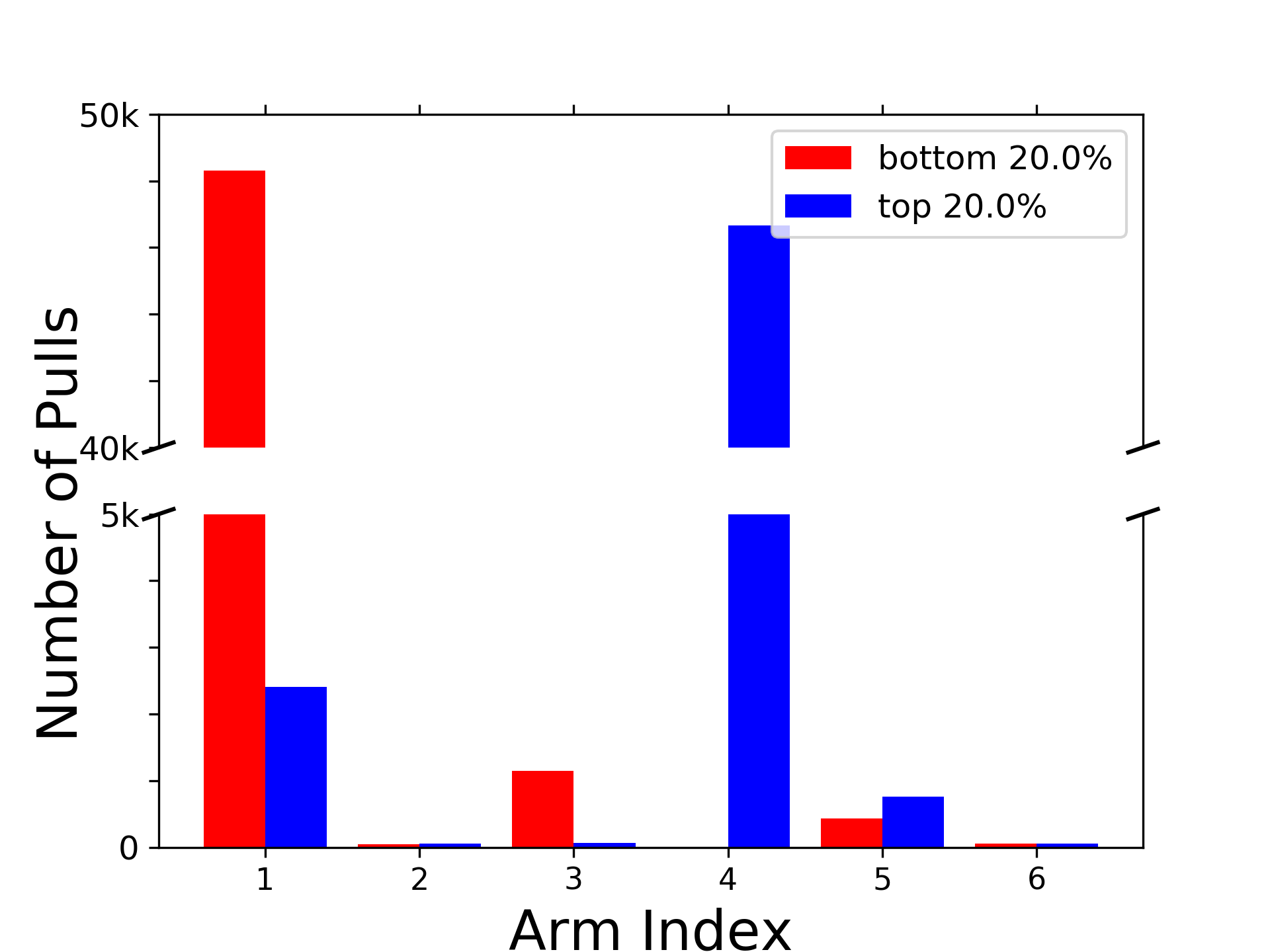
Fig. 4: Behavior of π⁡(L^t)\pi(\hat{L}_{t}) for given 𝝁\bm{\mu} and 𝒙\bm{x} shown in Figure 1(a).

We provide additional experiments with respect to a numerical evidence on a risk presented in Section II-C. It is worth closely investigating the failure of π⁡(L^t)\pi(\hat{L}_{t}) with Figure 1. Figure 4(a) presents the histogram of L^T\hat{L}_{T} at T=50​kT=50k. A sustainable portion of sample paths (1616 out of 100100; the first bin in Figure 4(a)) has the estimation L^T\hat{L}_{T} concentrated around the second steepest slope (0.10.1) in Figure 1(a). Figure 4(b) and 4(c) compare two groups of sample paths with the bottom-2020% or top-2020% values of L^T\hat{L}_{T} at T=50​kT=50k in Figure 4(a). As shown in Figure 4(b), the bottom-2020% group with under-estimated L^t\hat{L}_{t} misidentifies the second best arm 11 as the best arm and mainly contributes the linear regret. An explanation on such a catastrophic failures is provided in Figure 4(c) where the bottom-2020% group can hardly recover from the estimation error in L^t\hat{L}_{t}. Suppose that at certain iteration tt, the second best arm 11 (accidentally) has a much higher empirical mean than the others, i.e., μ^​(1)≫maxi=2,…,6⁡μ^​(i)≈0\hat{\mu}(1)\gg\max_{i=2,...,6}\hat{\mu}(i)\approx 0. Then, the value of L^t\hat{L}_{t} is much lower than LL as arm 11 is far from every other point. The underestimated L^t\hat{L}_{t} forces the algorithm overgeneralize and excessively reduces the exploration rate on arms 22-66 and also the chance of correcting L^t\hat{L}_{t}. The failure of π⁡(L^t)\pi(\hat{L}_{t}) simultaneously learning structure and minimizing regret motivates us to study a scenario of transfer learning.

F-B Numerical evaluation

(a) Incidences of 𝝁m\bm{\mu}_{m}’s (L=0.5L=0.5)
(b) Histogram of LmL_{m}’s (L=0.5L=0.5)
(c) Histogram of L^m\hat{L}_{m}’s (L=0.5L=0.5)
(d) Incidences of 𝝁m\bm{\mu}_{m}’s (L=5L=5)
(e) Histogram of LmL_{m}’s (L=5L=5)
(f) Histogram of L^m\hat{L}_{m}’s (L=5L=5)
Fig. 5: Examples and statistics of experienced tasks generated by the procedure in Section IV with L∈{0.5,5}L\in\{0.5,5\}
(a) Evolution of estimation over episodes (L=0.5L=0.5)
(b) Cumulative regret over episodes (L=0.5L=0.5)
(c) Evolution of estimation over episodes (L=5L=5)
(d) Cumulative regret over episodes (L=5L=5)
Fig. 6: Comparison of various estimators using the past experiences in Figure 5 for L∈{0.5,5}L\in\{0.5,5\}

We present additional experiments to compare the performance of estimators on different Lipschitz constant L∈{0.5,5}L\in\{0.5,5\}.

Setup. For numerical simulation, we consider Lipschitz structure Φ⁡(L)\Phi(L) with L∈{0.5,5}L\in\{0.5,5\}, K=6K=6 and 𝒙=(0,0.8,0.85,0.9,0.95,1)\bm{x}=(0,0.8,0.85,0.9,0.95,1). For each episode m∈[M=400]m\in[M=400] of length T=10,000T=10,000, we generate 𝝁m∈Φ⁡(L)\bm{\mu}_{m}\in\Phi(L) as shown in Section IV. For each of L=0.5L=0.5 and L=5L=5, Figures 5(a) and 5(d), respectively, show five 𝝁m\bm{\mu}_{m}’s generated from the generative procedure, and Figures 5(b) and 5(e), respectively, present the histogram of 400 LmL_{m}’s. For every estimator (stated below), for L∈{0.5,5}L\in\{0.5,5\}, we use the same sequence of L^m\hat{L}_{m}’s generated by π⁡(∞)\pi(\infty) that uses no continuity structures.

Stable estimator L^β\hat{L}_{\beta}. We compare four estimators on Lipschitz constant: three L^β\hat{L}_{\beta}’s with (β,εβ)∈{(0.5,0.05)(\beta,\varepsilon_{\beta})\in\{(0.5,0.05), (0.3,0.05)(0.3,0.05), (0.1,0.05)}(0.1,0.05)\} and L^max\hat{L}_{\max} which takes the maximum of L^m\hat{L}_{m}’s estimated previously. The histogram of empirical L^m\hat{L}_{m} is presented in Figures 5(b)  and 5(e). Figures 6(a)  and 6(c) compare the accuracy of estimators. As expected, for both L=0.5L=0.5 and L=5L=5, the most conservative estimation of L^max\hat{L}_{\max} has monotonically increasing estimation of LL as the past episodes piling up. Theoretically, L^max\hat{L}_{\max} can explode up to 1/Δ𝒙=201/\Delta_{\bm{x}}=20 in a finite number of episodes with positive probability. However, each of L^β\hat{L}_{\beta}’s is stabilizing the estimation on Lischiptz constant LL regardless of its value once we collected sufficient experiences, e.g., M>30M>30. Comparing the histograms of true LmL_{m}’s for different values of LL (Figures 5(b) and 5(e)), the portion of tight LmL_{m} for L=0.5L=0.5 is more than that for L=5L=5. Hence, when L=0.5L=0.5, we can obtain a safe estimation L^β≥L\hat{L}_{\beta}\geq L even for the aggressive choice of β=0.5\beta=0.5. However, when L=5L=5, the same choice of β\beta gives a risky estimation L^β≲L\hat{L}_{\beta}\lesssim L, in which padding some εβ\varepsilon_{\beta} may be helpful.

Cumulative regret. We present cumulative regret under various estimators in Figures 6(b) and 6(d). Note that the embedding of arm 1 is far from those of the other arms 22 to 66. Hence, we anticipate that the observations among the neighboring arms 22 to 66 are easily generalized to each other via Lipschitz continuity. In particular, the gain from Lipschitz continuity is much larger for L=5L=5 than L=0.5L=0.5 since the suboptimality gap Δ𝝁\Delta_{\bm{\mu}} can be larger for L=5L=5 than L=0.5L=0.5. In Figure 6(d), as discussed in our analysis, more accurate estimation of LL consequences greater reduction in regret. Employing small value of β\beta provides much conservative estimation of LL, but it can be too conservative to exploit the Lipschitz constant.