False vacuum decay in a two-dimensional black hole spacetimePreprint: KOBE-COSMO-21-02
Abstract
We study a false vacuum decay in a two-dimensional black hole spacetime background. The decay rate in the case that nucleation site locates at a black hole center has been calculated in the literature. We develop a method for calculating the decay rate of the false vacuum for a generic nucleation site. We find that the decay rate becomes larger when the nucleation site is close to the black hole horizon and coincides with that in Minkowski spacetime when the nucleation site goes to infinity.
I Introduction
The vacuum in the standard model of particle physics (SM) confirmed by the discovery of Higgs boson ATLAS:2012; CMS:2012 might be metastable depending on the top quark mass which has been yet completely fixed experimentally. The metastable false vacuum state must decay into the true vacuum Coleman:1977-1; Coleman:1977-2; Coleman:1980. Since the life time of the false vacuum in a flat spacetime is much longer than the age of the universe Chigusa:2017, it is believed that there is no apparent inconsistency in the SM. However, there might have been primordial black holes in the early universe. Therefore, it is necessary to know the decay rate of the false vacuum in the presence of black holes. Indeed, Hiscock pointed out that the black hole makes the life time of the false vacuum shorter Hiscock:1987. Recently, it is shown that the life time of the Higgs vacuum is less than the age of the universe in the presence of the small black holes Gregory:2013; Gregory:2015; Gregory:2015-2; Gregory:2016; Gregory:2016-2. Considering the Hawking evaporation of black holes, small black holes would be ubiquitous in the early universe. Thus, the Higgs vacuum might be unstable. If so, we need to go beyond the SM, namely, the instability suggests a new physics at the energy scale higher than the TeV scale Degrassi:2012; Gorsky:2014; Bezrukov:2014; Ellis:2015; Buttazzo:2013; Miro:2011; Chetyrkin:2012.
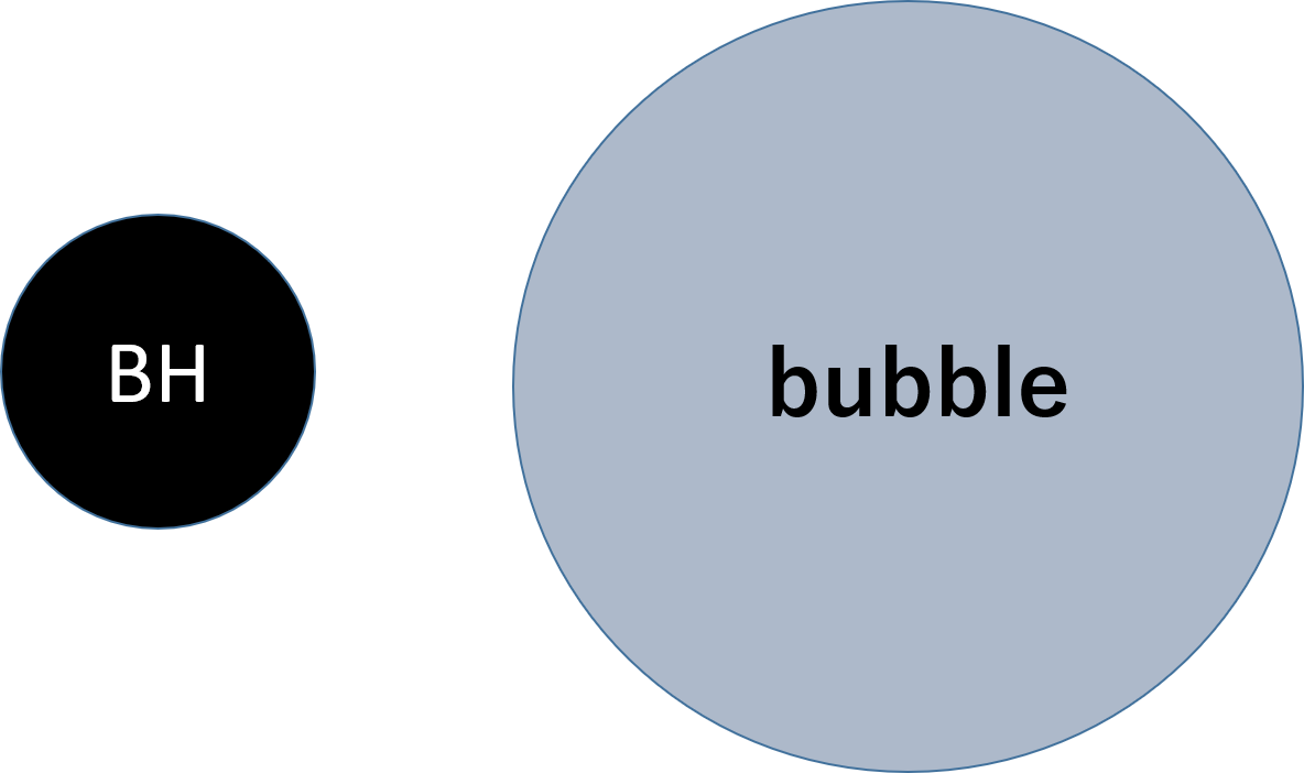
It should be noticed that there are two points to be clarified in previous computations of the decay rate of the false vacuum with black holes. First, in Hiscock:1987; Gregory:2013; Gregory:2015; Gregory:2015-2; Gregory:2016; Gregory:2016-2, the back-reaction of the false vacuum decay to spacetime geometry is taken into account and the black hole spacetime changes after tunneling. The validity of such a quantum gravitational picture is not apparent at least in the period around the electroweak phase transition. Second, no one has considered cases where a nucleation site of a true vacuum is away from the black hole (Fig.1). This is because there is a difficulty in investigating the false vacuum decay in the presence of a black hole. Indeed, the black hole breaks the translation symmetry and hence the dominant bubble shape away from a black hole is no more spherical. Note that it is worth investigating bubble nucleation away from black holes because the process is relevant to estimation of gravitational waves from bubble collisions Kosowsky:1992. In fact, the presence of black holes would change the nucleation rate and we need to take into account collisions between black holes and bubbles on top of the bubble collisions.
In this paper, as a first step, we consider the false vacuum decay in a two-dimensional black hole. To resolve the first issue, we take a semi-classical approach and consider the vacuum decay in a fixed black hole spacetime. As to the second issue, we consider two-dimensions where we can develop a new method by extending the formulation in Vakkuri:1996; Darme:2017 to calculate the decay rate. Using numerical calculations, we find the decay rate of the false vacuum is enhanced in the presence of a black hole in two-dimensions. The decay rate becomes larger when the nucleation site is close to the black hole horizon and coincides with that in Minkowski spacetime when the nucleation site goes to infinity.
The organization of the paper is as follows. In Sec.II, we briefly review how to calculate a decay rate of a false vacuum in Minkowski spacetime. Then, we introduce a new method for calculating a nucleation rate of a bubble nucleated at the center of a black hole and compare with previous researches. In Sec.III, we calculate the decay rate of the false vacuum for which nucleation site locates at a generic point. We find the fitting formula for a bubble formation which yields the decay rate through a bubble nucleation away from the black hole. For comparison, we also study the case of a four-dimensional spacetime by taking annular bubbles and show that the decay rate is also enhanced as in the case of a two-dimensional spacetime. Of course, the bubble with such a shape is not dominant one in four-dimensions but it is useful to see the tendency of the false vacuum decay in the presence of black holes. The final section is devoted to conclusion.
II Nucleation at the center of a black hole
In this section, we calculate a decay rate for a false vacuum decay when the nucleation site locates at the center of a black hole. Recently, this rate has been investigated in Gregory:2013 by using Israel junction conditions Israel:1966 to treat the dynamics of the bubble. In this paper, we use the fixed background. Hence, instead of the junction conditions, we extend a method for treating the dynamics of the bubble in Minkowski spacetime Vakkuri:1996; Darme:2017 to a two-dimensional Schwarzschild black hole spacetime.
II.1 False vacuum decay in Minkowski spacetime
Here, we briefly summarize the false vacuum decay in Minkowski spacetime. Let us consider the following action
| (1) |
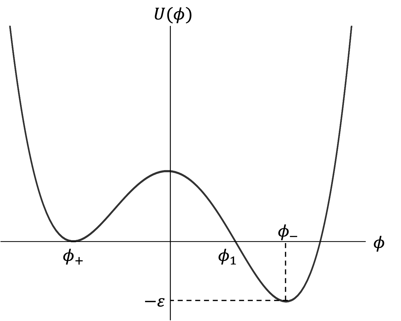
where the potential has two local minima (FIG.2). In this paper, we take these minima as follows
| (2) |
Here, is the difference of the energy density between the true and the false vacuum.
We can calculate the decay rate of the false vacuum as follows Coleman:1977-1;
| (3) |
where is the classical Euclidean action for the vacuum decay process and is that of the false vacuum. In this setup, vanishes and what we have to calculate is . The prefactor includes quantum corrections Coleman:1977-2. We focus on the leading contribution in this paper. In a two-dimensional Minkowski spacetime, the exponent is given by (see Appendix A),
| (4) |
where is the surface tension of the bubble wall.
II.2 False vacuum decay in black hole spacetime
Now, we move on to the black hole spacetime. We want clarify the effect of a black hole on the false vacuum decay process. The metric of the black hole is given by
| (5) |
where is the black hole mass and is the absolute value of a spatial position from the center. Here, we assumed the reflection symmetry with respect to . Now we put the bubble radius and divide the action into three parts
| (6) |
where , and are contributions from the wall, outside the bubble and inside the wall, respectively. Assuming that is static and homogeneous both inside and outside of the bubble, can be easily calculated as
| (7) |
where is a gravitational radius of the black hole. Since there is no matter inside the black hole, the volume of the black hole is subtracted. To calculate , we need several steps. First, using the spatial reflection symmetry, the action can be written as
| (8) |
Second, the tangent and normal vector of the wall is given by
| (9) |
where a dot denotes a derivative with respect to the time. Defining the following derivative operators
| (10) |
we obtain
| (11) |
We are now in a position to use the thin-wall approximation Coleman:1977-1(see Appendix A for more details). We envisage the situation that the energy is concentrated in the thin wall of the bubble and assume that
| (12) |
Thus, can be approximated as
| (13) |
The equation of motion is given by
| (14) |
Integrating this equation from the outside of the bubble to the wall, we obtain
| (15) |
Then can be calculated as
| (16) | |||||
In the thin wall approximation, we can deduce the relation
| (17) |
Therefore, we obtain
| (18) | |||||
where is the tension of the bubble wall (see (73));
| (19) |
Finally, we obtain the following effective action;
| (20) |
With the Wick rotation , the effective Euclidean action reads
| (21) |
where a prime denotes a derivative with respect to an Euclidean time .
Let us evaluate the decay rate of the false vacuum. The dynamics of the bubble wall in the Lorentzian spacetime can be deduced from the Hamiltonian derived from the action (20) as
| (22) |
Since the initial energy vanishes, from the energy conservation law, we have
| (23) |
From this, we obtain the following equation
| (24) |
Performing the Wick rotation , we can also obtain the Euclidean equation
| (25) |

In FIG. 3, we plotted the effective potential for various masses of black holes. The left zero point of corresponds to the location of the black hole horizon; . The right zero point of is an initial position of the bubble wall; . After the tunneling, the bubble wall appears at and expands rapidly.
First, we calculate the decay rate in the case of a Minkowski spacetime and check the consistency with the known result (4). From (25), we can derive an equation for the Minkowski spacetime
| (26) |
With the initial condition , we obtain
| (27) |
where . Note that the initial radius is the same as that derived in Appendix A. Substituting this solution into the Euclidean action (21) and integrating over , we obtain the exponent
| (28) | |||||
This coincides with the result of (4).

Now, for the Schwarzschild spacetime, the exponent is given by
| (29) |
where is the period of the solution of (25). We numerically evaluated and plotted it in FIG. 4. It turns out that the black hole makes the decay rate smaller than that in the Minkowski spacetime.
The present formulation can be extended to the 4-dimensional spacetime as shown in Appendix B. In this case, the decay rate is enhanced for small black holes (FIG. 5). This is consistent with the result in Gregory:2013. Thus, we have shown that the qualitative behavior of the decay rate depends on the dimensions when the nucleation site is located at the center of a black hole.

III Nucleation at a generic location
In this section, we consider the decay rate of the false vacuum when the nucleation site is located outside a black hole. There are two bubble walls which are represented by
| (30) |
In the previous section, we used the reflection symmetry to reduce the dynamics of two walls in both sides of the black hole to the dynamics of a single wall. In this section, however, we have to treat these two walls independently because of the lack of symmetry in the case of the bubble nucleation outside a black hole.
Let us investigate the dynamics of the bubble walls. Let us consider the following action
| (31) |
The metric is the same as (5). As in the last section, we can derive the effective action as follows
| (32) |
We have to follow the dynamics of two walls using a Hamilton formulation because it is difficult to obtain effective potentials from the energy conservation law. In a Lorentzian formalism, the Hamiltonian is given by
| (33) |
where is the Lorentzian canonical conjugate momentum for or . The Hamilton equations of motion are as follows;
| (34) | |||
| (35) |
where is either or . For the second equation, the minus sign is for and the other is for . From energy conservation law, we obtain
| (36) |
To make an analytic continuation, we choose the boundary conditions at the turning point as follows;
| (37) |
From (34), there are two choices for the wall of ; or and we choose the former to consider a bubble away from the black hole. Taking into account , the initial condition for the wall position Q must be . Then, the two initial conditions read
| (38) |
From and , we also obtain
| (39) |
Hence, one constant of integration is left in solutions of Eqs.(34) and (35). The single parameter determines the location where the bubble appears. Therefore, from (34), (35), (38) and (39), the Lorentzian dynamics of the bubble wall can be solved.
In an Euclidean region, the effective action reads
| (40) |
The Hamiltonian in this case is given by
| (41) |
where is the Euclidean canonical conjugate momentum for or . The Hamilton equations of motion are as follows;
| (42) | |||
| (43) |
To perform analytic continuation from the Euclidean solution into the Lorentzian solution, we choose the conditions at the transition point;
| (44) | |||
| (45) |
Therefore, from (42), (43), (44) and (45), the Euclidean dynamics of the bubble wall can be deduced.
III.1 A consistency check
To check the consistency, we calculate the decay rate of the false vacuum in the Minkowski spacetime (4). The Euclidean Hamilton equations of motion (42) and (43) become
| (46) | |||
| (47) |
These equations can be solved easily under the initial conditions ;
| (48) |
where is a constant of integration and . From (45), we see
| (49) |
Then, the constant represents the center of the bubble. Thus, the exponent is given by
| (50) | |||||
This is the same result as (4).
III.2 Decay rate for a generic nucleation site
Now, we are in a position to calculate the decay rate for generic cases. In the absence of a black hole, and have the same period. However, it is not true in the presence of a black hole (FIG. 6). This does not matter because the two walls contribute to the Euclidean action (40) independently.
First, we have numerically solved the dynamics of bubble walls. In FIG. 6, the trajectories of bubble walls for various masses of black holes with a specific initial locations of bubbles are plotted. We analytically continue Lorentzian solutions () and Euclidean solutions () at . After a bubble nucleation (), the bubble wall P falls into black hole horizon and the other wall Q goes to infinity at the speed of light in Schwarzschild spacetime. In the Minkowski case, the trajectories of and are symmetric. While, when the nucleation point of is close to the horizon, the trajectories become asymmetric in the black hole cases.

|

|

|
For the Schwarzschild black hole spacetime, the exponent is given by
| (51) |
where denotes the period of . We calculate the exponent numerically and find that the black hole enhances the decay rate for nucleation process of a bubble (FIG. 7). The decay rate is largest at the horizon and asymptotically approaches the result of Minkowski spacetime as the nucleation point goes to infinity. Note that small black holes make the decay rates larger Gregory:2013; Gregory:2015; Gregory:2015-2; Gregory:2016; Gregory:2016-2.

|

|
We shall find a fitting formula for the solutions. Notice that, in the absence of a black hole, the solutions (48) can be written as
| (52) |
In order to find a fitting formula, we take the ansatz in the Euclidean region
| (53) |
where is the half period of solutions and . We put these two parameters as follows
| (54) | |||||
| (55) |
where are fitting parameters calculated by least squares method. In the absence of a black hole, we should take the limits or . Using these ansatze, the decay rate (51) can be evaluated as
| (56) | |||||
where we performed the transformation of a variable in the integral. The decay rate obtained from a fitting formula shows a good agreement with the numerical calculation (FIG. 8). Thus, the fitting formula (53) is a good approximation for the dynamics of the bubble wall in the black hole spacetime.

|

|
III.3 Discussion
What we wanted to reveal is the effect of a black hole on the decay rate of the false vacuum in four-dimensions. In this subsection, we discuss a four-dimensional false vacuum decay.

As we already mentioned, it is not easy to solve the nucleation process in four-dimensions. As a modest first step, we consider the annular bubble in a four-dimensional black hole spacetime (FIG. 9). We extended the formulation in two-dimensions to four dimensions in Appendix B. Apparently, the annular bubble (FIG.9) does not describe a dominant process of the false vacuum decay. However, it is useful to see the tendency of gravitational effects on the decay process in a four-dimensional black hole spacetime.

From numerical calculations, we see the black hole also enhances the decay rate of the false vacuum even in four dimensions (FIG. 10). Therefore, it is expected that the black hole also enhanced the decay rate of the false vacuum through the dominant bubble nucleation process in a four-dimensional black hole spacetime.
IV Conclusion
We studied the false vacuum decay in a two-dimensional black hole spacetime. In particular, we considered the cases the bubble nucleates at a generic point in the black hole spacetime. We developed a method for calculating the decay rate in a fixed Schwarzschild black hole spacetime by extending the formulation in Vakkuri:1996; Darme:2017. Using numerical calculations, we showed that the black hole enhances the decay rate when the nucleation occurs outside of the black hole. The decay rate is maximized near the horizon and reduces to the one for a Minkowski spacetime at infinity. This is natural because away from the horizon the spacetime asymptotically approaches the Minkowski spacetime. Our finding indicates that it is worth investigating the decay rate of the false vacuum in a four-dimensional black hole spacetime in order to discuss gravitational waves from bubbles collisions and black hole bubble collisions Kosowsky:1992.
For future work, it is interesting to apply our method to other O(3) symmetric spacetimes such as Schwarzschild-deSitter black holes or charged black holes. We expect that the cosmological constant make the decay rate larger and the charge affects oppositely as in the previous works Gregory:2013; Gregory:2015-2. It is challenging to study the false vacuum decay in a four-dimensional black hole spacetime because the bubble outside the black hole horizon breaks the symmetry of the spacetime. It is also intriguing to consider rotating black holes Oshita:2019.
Acknowledgments
J. S. was supported by JSPS KAKENHI Grant Numbers JP17H02894 and JP20H01902.
Appendix A N dimensional bubble in Minkowski spacetime
In this appendix, we derive the decay rate in a N-dimensional Minkowski spacetime based on Coleman:1977-1.
Let us consider the following action
| (57) |
where the potential has two local minima (FIG.2). For simplicity, we take these minima as follows
| (58) |
In this setup, vanishes and we only have to treat . Performing the Wick rotation , we obtain the following Euclidean action
| (59) |
From this Euclidean action, the equation of motion for is derived as
| (60) |
where is the Laplacian for a (N-1)-dimensional Euclidean space. To derive a solution which contributes to a vacuum decay, we impose the following boundary conditions;
| (61) | |||
| (62) | |||
| (63) |
Next, we assume O(N) symmetry so that depends only on . Then, (59), (60), (61), (62) and (63) become
| (64) | |||
| (65) | |||
| (66) | |||
| (67) |
where is the surface area of a unit sphere. The solutions satisfying the boundary conditions (66) and (67) is called the bounce solution Coleman:1977-1.
Let us now show the existence of the bounce solution. There is a zero point of between and and we write it as . Since the Euclidean energy monotonously decreases;
| (68) |
will undershoot at when . If is very close to , the equation of motion (65) can be linearized as follows;
| (69) |
where . The solution is given by
| (70) |
where is the Gamma function and is the modified Bessel function of the first kind. If we put sufficiently close to , will stay around for long time . However, the damping force which is proportional to can be neglected at large and will overshoot at . Therefore, there must be intermediate initial position for which just comes to rest at after the infinite time .
From the above argument, of the bounce solution stays near for a long time and goes quickly to . Let us consider the behavior of near . For , we can neglect the damping force and the equation of motion becomes
| (71) |
where . This equation has the following solution;
| (72) |
The action for this solution is given by
| (73) | |||||
where is the surface tension of the bubble. Then the bounce solution is as follows;
| (74) |
The region where is called bubble. To obtain the decay rate, we assume that is sufficiently larger than the wall width of the bubble. This approximation is called the thin-wall approximation. Then, after substituting (74) into (64), we can divide the Euclidean action into three parts;
| (75) |
where () denotes outside (inside) of the bubble and is the contribution of the bubble wall. Using (73), we obtain
| (76) |
where is the volume of a unit sphere. Taking the Variation with respect to R
| (77) |
we obtain . Note that the thin-wall approximation can be stated quantitatively as follows;
| (78) |
We finally obtain the exponent
| (79) |
where we write down and explicitly. This is an extension of the result in Coleman:1977-1 to a N-dimensional Minkowski spacetime.
Appendix B N-dimensional effective action
In this appendix, we extend the effective actions (20) and (32) to a N-dimensional spacetime. In both cases, we assume O(N-1) symmetry for the spatial configuration of a scalar field. Note that an annular bubble is assumed for a generic nucleation. We can take the same method as the 2-dimensional cases to derive the effective actions in N-dimensional spacetime. The action (20) is extended to
| (80) |
and the action (32) is also extended to
| (81) |
where is the volume of a N-dimensional unit sphere and is the surface area of that. From these actions, the dynamics of the bubbles can be derived and we can calculate the decay rate by imposing the same boundary conditions as those in 2-dimensional spacetime.
References
- (1) G. Aad et al. , “Observation of a new particle in the search for the Standard Model Higgs boson with the ATLAS detector at the LHC,” Phys. Lett. B 716 (2012) 1-29. [arXiv:1207.7214 [hep-ex]].
- (2) S. Chatrchyan et al. , “Observation of a new boson at a mass of 125 GeV with the CMS experiment at the LHC,” Phys. Lett. B 716 (2012) 30. [arXiv:1207.7235 [hep-ex]].
- (3) S. R. Coleman, “Fate of the false vacuum. 1. Semiclassical Theory∗,” Phys. Rev. D 15 (1977) 2929-2936, Phys. Rev. D 16 (1977) 1248 (erratum).
- (4) C. G. Callan and S. R. Coleman, “Fate of the false vacuum. 2. First Quantum Corrections∗,” Phys. Rev. D 16 (1977) 1762-1768.
- (5) S. R. Coleman and F. D. Luccia, “Gravitational Effects on and of Vacuum Decay,” Phys. Rev. D 21 (1980) 3305.
- (6) S. Chigusa, T. Moroi, Y. Shoji, “State-of-the-Art Calculation of the Decay Rate of Electroweak Vacuum in Standard Model,” Phys. Rev. Lett. 119 211801 (2017) [arXiv:1707.09301 [hep-ph]].
- (7) W. A. Hiscock, “Can black holes nucleate vacuum phase transitions?,” Phys. Rev. D 35, (1987) 1161.
- (8) R. Gregory, I. G. Moss and B. Withers, “Black holes as bubble nucleation sites,” JHEP 03 (2014) 081 [arXiv:1401.0017 [hep-th]].
- (9) P. Burda, R. Gregory and I. Moss, “Gravity and the stability of the Higgs vacuum,” Phys. Rev. Lett. 115 (2015) 071303 [arXiv:1501.04937 [hep-th]].
- (10) P. Burda, R. Gregory and I. Moss, “Vacuum metastability with black holes,” JHEP 08 (2015) 114 [arXiv:1503.07331 [hep-th]].
- (11) P. Burda, R. Gregory and I. Moss, “The fate of the Higgs vacuum,” JHEP 06 (2016) 025 [arXiv:1601.02152 [hep-th]].
- (12) R. Gregory and I. G .Moss, “The Fate of the Higgs Vacuum,” PoS ICHEP2016 (2016) 344 [arXiv:1611.04935 [hep-th]].
- (13) G. Degrassi, S. D. Vita, J. E. Miro, J. R. Espinosa and G. F. Giudice, “Higgs mass and vacuum stability in the Standard Model at NNLO,” JHEP 08 (2012) 098 [arXiv:1205.6497 [hep-ph]].
- (14) A. Gorsky et al., “Is the Standard Model saved asymptotically by conformal symmetry?,” J. Exp. Theor. Phys. 120 (2015) 3, 344-353, Zh. Eksp. Teor. Fiz. 147 (2015) 399-409 [arXiv:1409.0492 [hep-ph]].
- (15) F. Bezrukov and M. Shaposhnikov, “Why should we care about the top quark Yukawa coupling?,” J. Exp. Theor. Phys. 120 (2015) 335-343, Zh. Eksp. Teor. Fiz. 147 (2015) 389-398 [arXiv:1411.1923 [hep-ph]].
- (16) J. Ellis, “Discrete Glimpses of the Physics Landscape after the Higgs Discovery,” J. Phys. Conf. Ser. 631 (2015) 1, 012001 [arXiv:1501.05418 [hep-ph]].
- (17) D. Buttazzo et al., “Investigating the near-criticality of the Higgs boson,” JHEP 12 (2013) 089 [arXiv:1307.3536 [hep-ph]].
- (18) J. E. Miro et al., “Higgs mass implications on the stability of the electroweak vacuum,” Phys. Lett. B 709 (2012) 222-228 [arXiv:1112.3022 [hep-ph]].
- (19) K. G. Chetyrkin and M. F. Zoller, “Three-loop -functions for top-Yukawa and the Higgs self-interaction in the Standard Model,” JHEP 06 (2012) 033 [arXiv:1205.2892 [hep-ph]].
- (20) A. Kosowsky, M. S. Turner, R. Watkins, “Gravitational waves from first order cosmological phase transitions,” Phys. Rev. Lett. 69 (1992) 2026-2029.
- (21) E. K. Vakkuri and P. Kraus, “Tunneling in a time dependent setting,” Phys. Rev. D 54 (1996) 7407-7420 [arXiv:hep-th/9604151 [hep-th]].
- (22) L. Darmé, J. Jaeckel and M. Lewicki, “Towards the fate of the oscillating false vacuum,” Phys. Rev. D 96 (2017) 5, 056001 [arXiv:1704.06445 [hep-th]].
- (23) W. Israel, “Singular hypersurfaces and thin shells in general relativity,” Nuovo Cimento Soc. Ital. Phys. B 44, 4349.
- (24) N. Oshita, K. Ueda, M. Yamaguchi, “Vacuum decay around spinning black holes,” JHEP 01 (2020) 015 [arXiv:1909.01378 [hep-th]].