Modeling and simulating the excited-state dynamics of a system with condensed phases: A machine learning approach

We consider the situations in which an exciton or electron transfer system interacts with molecular environments that give rise to dissipation and fluctuation in the system. The Hamiltonian of the system is expressed as

where the $j$th exciton or electron states with energies $\hbar\omega_{j}$ are represented by bra and ket vectors as $|j\rangle$ and $\langle j|$. The interaction energy between the $j$th and $k$th states is described by $\hbar\Delta_{jk}$. In our model, each state is coupled to a different molecular environment (labeled as $a$) that is treated as $N_{a}$ harmonic oscillators. The total Hamiltonian is then given by

where the momentum, position, mass, and frequency of the $l$th oscillator in the $a$th bath are given by $\hat{p}_{l}^{a}$, $\hat{x}_{l}^{a}$, $m_{l}^{a}$, and $\omega_{l}^{a}$, respectively. The system part of the system-bath interaction is expressed as

where $V_{jk}^{a}$ is the coupling constant for the $a$th bath between the $j$ and $k$ states. The $a$th heat bath can be characterized by the spectral distribution function (SDF), defined as

and the inverse temperature is $\beta\equiv 1/k_{\mathrm{B}}T$, where $k_{\mathrm{B}}$ is the Boltzmann constant. Various environments, for example, those consisting of nanostructured materials, solvents, and protein molecules, can be modeled by adjusting the form of the SDF. For the heat bath to act as an unlimited heat source possessing an infinite heat capacity, the number of heat-bath oscillators $N_{a}$ is effectively made infinitely large by replacing $J_{a}(\omega)$ with a continuous distribution. The above model has been frequently used in the analysis of photosynthetic systems,Strümpfer and Schulten 2009; Strümpfer and Schulten 2011; Strümpfer and Schulten 2012; Ishizaki and Fleming 2009; Olbrich et al. 2011; Raszewski et al. 2005; Renger et al. 2012; Müh et al. 2015; Müh et al. 2017; Gelzinis et al. 2017; Fujihashi et al. 2015; Novoderezhkin et al. 2011; Novoderezhkin et al. 2015; Gelzinis et al. 2013; Adolphs and Renger 2006 electron transfer,Garg et al. 1985; Wolynes 1987; Yan et al. 1988; Tanaka and Tanimura 2009; Tanaka and Tanimura 2010 DNA,Sim and Makri 1997; Sim 2004; Dijkstra and Tanimura 2010 and solar battery systems.Gélinas et al. 2014; Zirzlmeier et al. 2015; Tamura and Burghardt 2013; Huix-Rotllant et al. 2015; Oviedo-Casado et al. 2017; Cainelli and Tanimura 2021

We next consider the pigments in a molecular system, whose electric excitation or exciton states are described by Eq. (1). The electric states of the pigments depend on the configurations of the surrounding atoms at time $t$. The time evolution of the excited states of the system and environmental molecules are described by QM/MM simulations. Because our goal in constructing a system-bath model is to perform a full quantum simulation of the entire system, we should use quantum molecular dynamics (MD) simulations to provide data on the basis of all atomic coordinates. In practice, however, it is impossible to consider large environmental degrees of freedom accurately from a quantum mechanical perspective. Fortunately, we expect that we already have reasonable SDFs for quantum simulation, even though we evaluated them using the classical MD simulation. Such evaluations were conducted utilizing an ensemble of molecular trajectories that exhibit a Gaussian distribution in which the difference between the quantum and classical trajectories is expected to be minor. Further, the dynamics of harmonic oscillators are identical in both the classical and harmonic cases because both the classical and quantum Liouvillian for the $l$th oscillator in the $a$th bath are expressed as ${\hat{L}}_{l}^{a}=-({p_{l}^{a}}/{m_{l}^{a}})({\partial}/{\partial x_{l}^{a}})-m(\omega_{l}^{a})^{2})({\partial}/{\partial p_{l}^{a}})$. We thus use the classical MD simulation technique to acquire the atomic coordinates of the pigments and the molecular environment. We then conduct quantum chemistry calculations to obtain the desired electronic states, typically the highest occupied molecular orbital (HOMO) and lowest unoccupied molecular orbital (LUMO) states of the pigments as a function of time. The excited energy of the $j$th pigment is denoted by $\epsilon_{jj}(t)$, and the interaction energy between the $j$th and $k$th pigments that includes the bath-induced fluctuation is denoted by $\epsilon_{jk}(t)$; these values can be obtained using any kind of numerical program for quantum chemistry calculations. If the main system is too large to enable evaluation of all electronic states, we evaluate the site energy $\epsilon_{jj}(t)$ and the interaction energy $\epsilon_{jk}(t)$ separately. From the calculated $\epsilon_{jj}(t)$ and $\epsilon_{jk}(t)$, we evaluate the system-bath coupling strength in $\hat{V}_{jk}^{a}$ and its SDF, in addition to the excitation energy $\hbar\omega_{j}$ and the interaction energy $\Delta_{jk}$, based on the machine learning approach.

While the SDFs evaluated based on the MD simulations are temperature dependent, the SDFs for the HOB are temperature independent; we therefore eliminate the temperature dependence of optimized parameters, assuming that the sampled MD trajectories exhibit canonical ensembles at finite temperatures.

For $n$ exciton or electronic excitation sites, we express the simulated data in terms of $\epsilon_{jk}(t)$ when describing the excited and site-site interaction energies of interest obtained from the QM/MM simulation. The learning Hamiltonian is then expressed as

We then attempt to reproduce the trajectories of $\epsilon_{jk}(t)$ for the total Hamiltonian, Eq. (2.1), with Eqs. (1) and (3). Although the system-bath model considers an infinite number of degrees of freedom, here, we employ a finite number of bath oscillators to estimate the SDFs. Then, the sampling used for machine leering training is considered the average of the classical bath oscillators for a certain selection of the system and system-bath parameters. The site energy and interaction energy can be expressed as

and

respectively, where $\delta_{jk}(t)$ is expressed in terms of the linear function of the bath coordinates as

Here, the $a$th bath coordinate for the $jk$ site is described as a function of time as

where $A^{a}_{jk}$ and $\phi^{a}_{jk}$ are the amplitude and phase of the $a$th bath oscillator for the $jk$ site, respectively. The phase $\phi^{a}_{jk}$ is randomly chosen to avoid recursive oscillator motion. Although we can consider such correlated modes separately by introducing additional baths, here, we assume that the influences of the individual bath modes are all independent and that the correlations between the fluctuations among different modes can be ignored.

From Eqs. (8) and (9), $\delta_{jk}(t)$ can be expressed as

where

and we treat the system-bath coupling parameters as the product of these two variables. In the machine learning context, the bath parameters and the system-bath interactions are expressed as a set of latent variables, defined as

where $\left\{...\right\}$ is the set of system and bath parameters. The trajectories of $\epsilon_{jj}(t)$ and $\epsilon_{jk}(t)$, obtained from the QM/MM calculations, are described as the vibrational motions of the pigment molecule and the surrounding molecules. We then assume that the probability distribution of the pure state energy $\lambda_{i}$ is determined based on a Gaussian process and is described by a set of bath parameters $\alpha^{a}_{jk}$ and $\phi^{a}_{jk}$ by optimizing the probability distribution defined as

which represents the marginalization of the phase of the oscillators $\phi^{a}_{jk}$ that is introduced to avoid trapping in a local minimal state due to the gradient method. Here, $P(\phi^{a}_{jk})$ is the uniform distribution of $[0,2\pi)$ and

where $E_{i}\equiv E_{i}(\theta;\phi^{a}_{jk})$ is the predicted energy as a function of the parameter set $\theta$ and initial phase $\phi^{a}_{jk}$ for the model Hamiltonian, Eq. (5), and $\sigma$ is the error width. Our goal in employing a machine learning method is to choose the optimal parameter set in $E_{i}(\theta;\phi^{a}_{jk})$ that maximizes the probability distribution for given data $\lambda_{i}$. Among several optimization methods, we use the maximum likelihood method (MLE), where the loss function is expressed in terms of the negative log of the probability as

To find the maximum value of $L$, we employ the Adam gradient method for optimization of the parameter set as

where $\gamma$ is the learning rate. In this way, we obtain the $J_{jk}$ element of the SDF for the $jk$ site. Because the energy distribution of each bath oscillator $E^{a}_{jk}=\frac{1}{2}m^{a}_{jk}\left(\omega^{a}_{jk}\right)^{2}$ is assumed to obey a canonical ensemble, the oscillator amplitude can be expressed as

Integrating Eqs. (11) and (17) into Eq. (4), we obtain

Because $J_{jk}(\omega)$ rapidly changes over time in accordance with the structural changes in the pigment molecules and environments, we evaluate $J_{jk}(\omega)$ by averaging the different sample trajectories. From a mathematical perspective, $c_{jk}$ is the frequency domain expression of the time domain data, and $J_{jk}(\omega)$ can be obtained by averaging the power spectra $c_{jk}^{2}$ using the Wiener-Khinchin theorem.

It should be noted that the absolute intensity of $J_{jk}(\omega)$ cannot be determined in the framework of the present study because, for simplicity, we do not evaluate the dipole moment of this complex material; we evaluate the intensity of $J_{jk}(\omega)$ from the width of the experimentally obtained linear absorption spectrum.

We now demonstrate our numerical approach for a dimer of identical indocarbocyanine molecules.Halpin et al. 2014 Figure 1 displays the structure of the pigment molecule. The ground and excited states of each pigment are expressed as $|0\rangle_{j}$ and $|1\rangle_{j}$ for $j=1$ and 2, respectively. The ground state energies are each set to zero. The system Hamiltonian is then expressed as

where $\omega_{0}$ is the excitation energy of a pigment and $\Delta$ is the interaction energy between the dimers. By diagonalizing $H$, we obtained the eigenvalues $\omega_{k}$ for the $k=+$ and $-$ eigenstates of $|1+\rangle=(|1\rangle_{1}|0\rangle_{2}+|0\rangle_{1}|1\rangle_{2})/\sqrt{2}$ and $|1-\rangle=(|1\rangle_{1}|0\rangle_{2}-|0\rangle_{1}|1\rangle_{2})/\sqrt{2}$, respectively, as

The excitation energy and interaction energy fluctuations as functions of time, arising from intramolecular motions of the pigment and intermolecular motions of surrounding molecules, are expressed as $\delta\omega_{\pm}(t)$ and $\delta\Delta(t)$, respectively. These functions are evaluated based on the quantum chemistry calculations for given atomic trajectories of the entire molecular system determined by MD simulations.

In our model, because each exciton state is delocalized and the effects of the environmental modes are site specific, we employ an individual heat bath expressed as the sum of site-specific oscillators to describe the energy fluctuation at each exciton site. The distribution of the exciton-oscillator coupling strength is then evaluated based on the machine learning approach. Although it is possible to introduce a global heat bath to induce low-frequency environmental modes that are coupled to multiple exciton states, we find that such effects are not significant in the present case. Therefore, the excitation energy and interaction energy fluctuations are expressed as

and

where $c^{a}_{bm}$ is the amplitude (scaled by $\alpha$, as described in Eq. (11)) and $\phi^{a}_{bm}$ is the initial phase of the $a$th oscillator for the state indices $b=11$ (or $22$) and $12$. We introduce the localization weight functions $w_{\pm,m}(t)$ and $w_{\Delta}(t)$, as obtained from the diagonalization of the pigment-based Hamiltonian, expressed in Eq. (3.1), to describe the pigment-specific environment effects in the delocalized exciton state representation. These localization weight functions are evaluated based on the electronic states of the pigment $m=1$ and $2$ established by the atomic orbitals (AO) obtained from quantum chemistry calculations.

Thus, the targeting eigenenergies to be described by the system-bath model, $\lambda_{\pm}(t;\theta)$, are expressed as

where $\theta$ is a set of parameters $\theta=\left(\omega_{0},\left\{c^{a}_{\pm,m}\right\},\Delta,\left\{c^{a}_{\Delta}\right\}\right)$. As learning data, we compute the exciton energy $E_{\pm}(t)$, the molecular orbital (MO) coefficients for each exciton state, and wavefunctions (atomic orbital (AO) coefficients for each MO) from quantum chemistry calculations for the given atomic coordinates as a function of time. Additionally, the movements of all atoms in the system are evaluated from the classical MD simulation. Using these data, we optimize the set of parameters $\theta$. To evaluate the weight function $w_{k,m}(t)$, we calculate the exciton and hole populations $p_{k,m}^{ex}(t)$ and $p_{k,m}^{h}(t)$ that are obtained as the summation of the absolute square of the AO coefficients, which are evaluated from the AO coefficients involved in the MO in pigment $m$ for excited state $k$. The weight function is then evaluated as $w_{k,m}(t)=p_{k,m}^{ex}(t)p_{k,m}^{h}(t)$ and $w_{\Delta}(t)=\sum_{k=\pm}\left(p_{k,1}^{h}(t)p_{k,2}^{ex}(t)+p_{k,2}^{h}(t)p_{k,1}^{ex}(t)\right)$. As these definitions indicate, the exciton states are localized when $w_{\pm,m}$ is close to 1, whereas the exciton states are distributed among the pigments when $w_{\Delta}$ is close to 1.

To optimize the system and bath parameter set, we minimize the loss function

where $E^{n}_{-}(t)$ and $E^{n}_{+}(t)$ are the lowest ($\left|1-\right>$) and 2nd lowest ($\left|1+\right>$) excitation energies, and the index $n$ indicates the $n$th sample. Using the MLE method, we optimize $c^{a}_{\omega_{0}m}$ and $c^{a}_{\Delta}$ for each time series as a sample set. To apply the machine learning algorithm, the time series of the tuple $(E^{n}_{-}(t),E^{n}_{+}(t),w^{n}_{k,m}(t))$ are regarded as the input feature variables. In the indocarbocyanine case, the two pigments are symmetric, and the bath SDFs for each pigment are considered to be identical. Therefore, we use the averaged value $c^{a}_{\omega_{0}}=(c^{a}_{\omega_{0}1}+c^{a}_{\omega_{0}2})/2$. We then evaluate $J_{jj}(\omega)(j=1,2)$ and $J_{12}(\omega)$, namely, $J(\omega)$ for $\omega_{0}$ and $\Delta$, from $c^{a}_{\omega_{0}}$ and $c^{a}_{\Delta}$, respectively, using Eq. (18).

A commonly used approach for evaluating the SDFs of $\epsilon_{ij}(t)$ utilizes the Fourier transformation of the autocorrelation function expressed as $\mathcal{F}\left[\left<\delta\epsilon_{ij}(0)\delta\epsilon_{ij}(t)\right>\right]$, where $\delta\epsilon_{ij}(t)\equiv\epsilon_{ij}(t)-\left<\epsilon_{ij}\right>$. In the actual calculation, the time series $\epsilon_{ij}^{n}(t)$, where $n$ is the sample index, is evaluated as the average of the autocorrelation function expressed as

where $N$ is the total sample number. We then obtain the SDF as

Alternatively, using Wiener-Khinchin’s theorem for stationary random processes, we can obtain the SDF as an average of power spectrum $P^{n}_{ij}(\omega)=\left|\mathcal{F}\left[\epsilon_{ij}(t)\right]\right|^{2}$ as

Although this Fourier-based approach is simple and straightforward, for the system-bath Hamiltonian, the obtained SDFs are not necessarily the optimal choice for describing the QM/MM data because the exciton and interaction energies are mutually dependent on each other; thus, $J_{ij}(\omega)$ and $J_{ik}(\omega)$ cannot be evaluated separately. In the machine learning approach, however, it is possible to optimize not only $J_{ij}(\omega)$ and $J_{ik}(\omega)$ but also $\omega_{0}$ and $\Delta$ without assuming explicit relationships between the SDFs and the system parameters. Moreover, if necessary, we can introduce additional conditions for optimization of the SDFs and system parameters because we employed $w_{k,m}(t)$ to account for the effects of the indocarbocyanine dimer exciton localization.

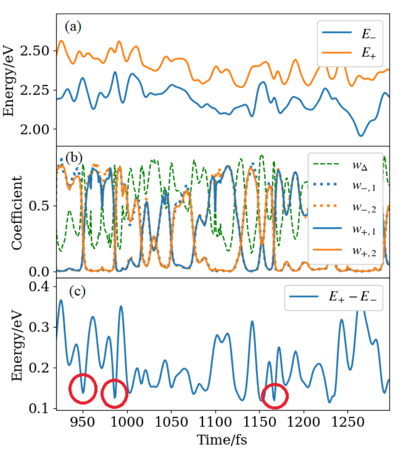
Representative examples of the prepared dataset are plotted in Fig. 2. The abrupt change in the exciton energies in Fig. 2(b) occurs due to the exciton transfer between pigments 1 and 2 that takes place in the time period of 10-100 fs. As illustrated in Fig. 2(c), the difference in the exciton energies $E_{+}-E_{-}$ exhibits minima in accordance with respect to the exciton transfer processes. As depicted by the red circles in Fig. 2(c), although such minimal points are significantly narrower and deeper than the minimal point caused by energetic fluctuation, it is difficult to separate the effects of exciton transfer from the energy fluctuation due to environmental motions. By introducing the localization weight functions $w_{\pm,m}(t)$ and $w_{\Delta}(t)$ in Eqs. (21) and (22) to eliminate the effects of the nonenvironmental origin involved in the learning trajectories, we can stabilize and enhance the efficiency of the machine learning process.

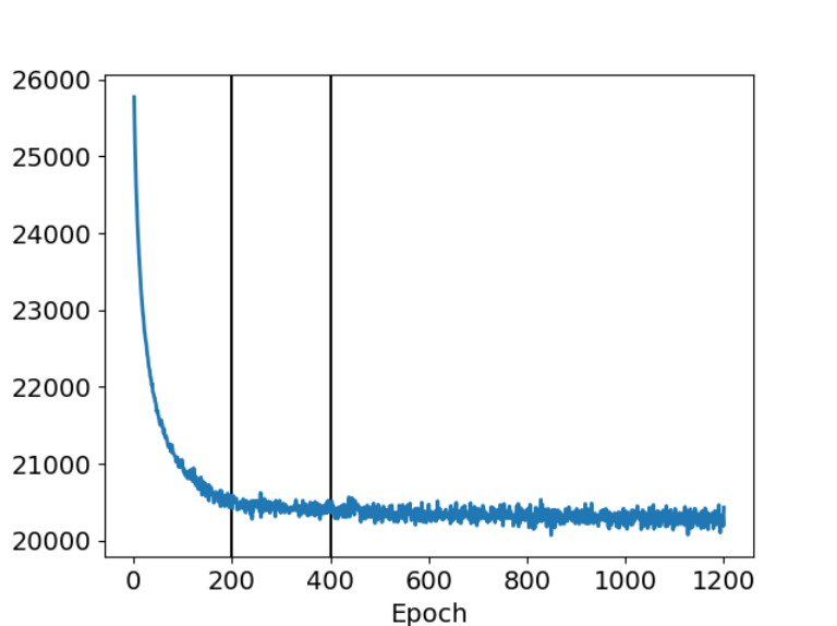
In Fig. 3, we depict the learning curve of the loss function, as defined in Eq. (3.1). Upon gathering random samplings of $\phi$, the loss function converged monotonically to a certain positive value, which demonstrated the efficiency of the present algorithm. The initial parameter values of the excitation energy and the interaction energy were set as $\omega_{0}$ = 17736 cm^-1 and $\Delta$ = 1004 cm^-1, whereas the optimized values of the excitation energy and the interaction energy were given by $\omega_{0}$ = 17794 cm^-1 and $\Delta$ = 963 cm^-1, which are closer to the values that fit the experimentally obtained spectra.Halpin et al. 2014 Here, to avoid overfitting problems, we employed the early-stopping technique (see Appendix B).

In Fig. 4, we display the results of SDFs for the excitation energy $J_{11}(\omega)$ ($=J_{22}(\omega)$) and the interaction energy $J_{12}(\omega)$. Various intermolecular modes below 2000 cm^-1 are observed as prominent sharp peaks near 450, 570, 1185, 1393, 1541, 1791, 1842, and 1923 cm^-1. In the region above 2000 cm^-1, only two tiny peaks are observed at approximately 3000 cm^-1 and 3850 cm^-1. The normal mode analysis (B3LYP/def-SV(P)) indicates that these peaks under 3300 cm^-1 arise from the intramolecular modes of the indocarbocyanine dimer, whereas the peak at 3850 cm^-1 arises from a molecular vibration of the solvent methanol molecules. We found that each sharp peak can be fitted by the Brownian spectral distribution,Tanaka and Tanimura 2009; Tanaka and Tanimura 2010 whereas the broadened background peak in the range from 0 to 2000 cm^-1 corresponds to the intramolecular modes fitted by the Drude-Lorentz distribution.Tanimura 2012 The intensities of the peaks in $J_{12}(\omega)$ are considerably weaker than those in $J_{11}(\omega)$: only the peaks near 456, 562, 1840 and 1920 cm^-1 are identified. As we expected, the intermolecular peak positions are governed by the classical MD simulation, whereas the heights of these peaks are predominately governed by the quantum chemistry calculation.

To verify the descriptions of the obtained SDFs and system parameters, we computed the linear absorption and two-dimensional electronic spectra (2DES), for the cases in which the experimentally obtained spectra were available.Halpin et al. 2014 In general, these spectra should be calculated in the framework of open quantum dynamics that considers the complex interactions between the exciton sites. However, for demonstration purposes here, we employ the analytical expressions for response functions, ignoring the transitions to the state that are usually forbidden. The details of these calculations are presented in Appendix A.

The linear absorption spectrum calculated from Eqs. (A.1 ) and A is presented in Fig. 6. Here, the calculated peak is fitted by the Gaussian function $\lambda\exp\left[-\left(({\omega-\omega_{c}})/{\gamma}\right)^{2}\right]$, where the amplitude, central frequency, and width are $\lambda=351$, $\omega_{c}=18583\mathrm{cm}^{-1}$, and $\gamma=464\mathrm{cm}^{-1}$, respectively. Note that we could not determine the absolute SDF intensities because, for simplicity, we did not calculate the amplitude of the dipole operator. Here, we chose to use the intensity of $J_{11}(\omega)$ to fit the experimentally obtained signal. As presented in Fig. 6, we observe a single broadened absorption peak at $\omega_{0}+\Delta$ corresponding to the transition between $|00\rangle$ and $|1+\rangle$, while the transition between $|00\rangle$ and the state $|1-\rangle$ is forbidden (see Fig. 5). Although the experimentally observed linear absorption spectrum exhibits a $0-1$ phonon sideband peak near $\omega=19500\mathrm{cm}^{-1}$, here, we observe this phenomenon only as an asymmetry of the Gaussian peak in the high-frequency region.

The 2D correlation electronic spectra calculated using the analytical expressions of the response function (Eqs. (A.5 ) -A.7 ) Tanimura and Mukamel 1995 are presented in Fig 7. At $t_{2}=0$ fs, only one peak stretched near the $\omega_{1}=\omega_{3}$ line, arising from the $|00\rangle\rightarrow|1+\rangle$ transition, is observed. At $t_{2}=10$, $25$, and $40$ fs, the peak is elongated in the low-frequency $\omega_{1}$ direction due to a shift in the eigenenergy caused by the heat-bath-induced exciton-exciton interaction described by $J_{12}(\omega)$. Because the system-bath interaction we considered here is non-Markovian and its effects appear only after a period longer than the inverse correlation time of noise, we do not observe such heat-bath effects for a small $t_{2}$. Then, at approximately $t_{2}=70$ fs, the off-diagonal peak near $(\omega_{1},\omega_{3})=(17800,20000)$, in units of cm^-1, corresponding to the transition between $|1+\rangle\rightarrow|11\rangle$ is observed, whereas the peak along the $\omega_{1}=\omega_{3}$ line shifts to $(\omega_{1},\omega_{3})=(21000,20000)$ due to the transition between $|00\rangle\rightarrow|1+\rangle$ that arises from the exciton-exciton interaction described by $\Delta$ and $J_{12}(\omega)$. As $t_{2}$ increases, the intensities of these two peaks oscillate as a result of the population transitions among $|10\rangle$, $|1+\rangle$, and $|11\rangle$ caused by $\Delta$ and $J_{12}(\omega)$. This phenomenon was also observed experimentally.Halpin et al. 2014 The appearance of this oscillatory feature at a finite period in $t_{2}$ indicates the importance of the off-diagonal heat bath, whose modeling is not easy in the framework of the existing approach.

While the off-diagonal peak still exhibits oscillatory motion at $t_{2}\geq 100$ fs, the peak profile gradually elongates in the $\omega_{1}=\omega_{3}$ direction due to the inhomogeneous broadening that arises from the diagonal bath modulation described by $J_{11}(\omega)$ and $J_{22}(\omega)$.Tanimura 2006

References

- May and Kühn (2003) May, V.; Kühn, O. Charge and Energy Transfer Dynamics in Molecular Systems; Wiley-VCH, 2003.
- Schröter et al. (2015) Schröter, M.; Ivanov, S.; Schulze, J.; Polyutov, S.; Yan, Y.; Pullerits, T.; Kühn, O. Exciton–vibrational coupling in the dynamics and spectroscopy of Frenkel excitons in molecular aggregates. Physics Reports 2015, 567, 1–78.
- Kreisbeck et al. (2014) Kreisbeck, C.; Kramer, T.; Aspuru-Guzik, A. Scalable High-Performance Algorithm for the Simulation of Exciton Dynamics. Application to the Light-Harvesting Complex II in the Presence of Resonant Vibrational Modes. J. Chem. Theory Comput. 2014, 10, 4045–4054.
- Lee and Coker (2016) Lee, M. K.; Coker, D. F. Modeling Electronic-Nuclear Interactions for Excitation Energy Transfer Processes in Light-Harvesting Complexes. J. Phys. Chem. Lett. 2016, 7, 3171–3178.
- Kreisbeck and Kramer (2012) Kreisbeck, C.; Kramer, T. Long-Lived Electronic Coherence in Dissipative Exciton Dynamics of Light-Harvesting Complexes. J. Phys. Chem. Lett. 2012, 3, 2828–2833.
- Strümpfer and Schulten (2009) Strümpfer, J.; Schulten, K. Light harvesting complex II B850 excitation dynamics. J. Chem. Phys. 2009, 131, 225101.
- Strümpfer and Schulten (2011) Strümpfer, J.; Schulten, K. The effect of correlated bath fluctuations on exciton transfer. J. Chem. Phys. 2011, 134, 095102.
- Strümpfer and Schulten (2012) Strümpfer, J.; Schulten, K. Excited state dynamics in photosynthetic reaction center and light harvesting complex 1. J. Chem. Phys. 2012, 137, 065101.
- Olbrich et al. (2011) Olbrich, C.; Strümpfer, J.; Schulten, K.; Kleinekathöfer, U. Quest for Spatially Correlated Fluctuations in the FMO Light-Harvesting Complex. J. Phys. Chem. B 2011, 115, 758–764.
- Ishizaki and Fleming (2009) Ishizaki, A.; Fleming, G. R. On the adequacy of the Redfield equation and related approaches to the study of quantum dynamics in electronic energy transfer. J. Chem. Phys. 2009, 130, 234110.
- Raszewski et al. (2005) Raszewski, G.; Saenger, W.; Renger, T. Theory of Optical Spectra of Photosystem II Reaction Centers: Location of the Triplet State and the Identity of the Primary Electron Donor. Biophys. J. 2005, 88, 986–998.
- Renger et al. (2012) Renger, T.; Klinger, A.; Steinecker, F.; Schmidt am Busch, M.; Numata, J.; Müh, F. Normal Mode Analysis of the Spectral Density of the Fenna–Matthews–Olson Light-Harvesting Protein: How the Protein Dissipates the Excess Energy of Excitons. J. Phys. Chem. B 2012, 116, 14565–14580.
- Müh et al. (2015) Müh, F.; Plöckinger, M.; Ortmayer, H.; Schmidt am Busch, M.; Lindorfer, D.; Adolphs, J.; Renger, T. The quest for energy traps in the CP43 antenna of photosystem II. J. Photochem. Photobiol., B 2015, 152, 286–300.
- Müh et al. (2017) Müh, F.; Plöckinger, M.; Renger, T. Electrostatic Asymmetry in the Reaction Center of Photosystem II. J. Phys. Chem. Lett. 2017, 8, 850–858.
- Gelzinis et al. (2017) Gelzinis, A.; Abramavicius, D.; Ogilvie, J. P.; Valkunas, L. Spectroscopic properties of photosystem II reaction center revisited. J. Chem. Phys. 2017, 147, 115102.
- Fujihashi et al. (2015) Fujihashi, Y.; Fleming, G. R.; Ishizaki, A. Impact of environmentally induced fluctuations on quantum mechanically mixed electronic and vibrational pigment states in photosynthetic energy transfer and 2D electronic spectra. J. Chem. Phys. 2015, 142, 212403.
- Novoderezhkin et al. (2011) Novoderezhkin, V. I.; Romero, E.; Dekker, J. P.; van Grondelle, R. Multiple Charge-Separation Pathways in Photosystem II: Modeling of Transient Absorption Kinetics. Phys. Chem. Chem. Phys. 2011, 12, 681–688.
- Novoderezhkin et al. (2015) Novoderezhkin, V. I.; Romero, E.; van Grondelle, R. How exciton-vibrational coherences control charge separation in the photosystem II reaction center. Phys. Chem. Chem. Phys. 2015, 17, 30828–30841.
- Gelzinis et al. (2013) Gelzinis, A.; Valkunas, L.; Fuller, F. D.; Ogilvie, J. P.; Mukamel, S.; Abramavicius, D. Tight-binding model of the photosystem II reaction center: application to two-dimensional electronic spectroscopy. New J. Phys. 2013, 15, 075013.
- Adolphs and Renger (2006) Adolphs, J.; Renger, T. How Proteins Trigger Excitation Energy Transfer in the FMO Complex of Green Sulfur Bacteria. Biophys. J. 2006, 91, 2778–2797.
- Garg et al. (1985) Garg, A.; Onuchic, J. N.; Ambegaokar, V. Effect of friction on electron transfer in biomolecules. J. Chem. Phys. 1985, 83, 4491.
- Wolynes (1987) Wolynes, P. G. Dissipation, tunneling, and adiabaticity criteria for curve crossing problems in the condensed phase. J. Chem. Phys. 1987, 86, 1957.
- Yan et al. (1988) Yan, Y. J.; Sparpaglione, M.; Mukamel, S. Solvation dynamics in electron-transfer, isomerization, and nonlinear optical processes: a unified Liouville-space theory. J. Phys. Chem. 1988, 92, 4842–4853.
- Tanaka and Tanimura (2009) Tanaka, M.; Tanimura, Y. Quantum Dissipative Dynamics of Electron Transfer Reaction System: Nonperturbative Hierarchy Equations Approach. J. Phys. Soc. Jpn. 2009, 78, 073802.
- Tanaka and Tanimura (2010) Tanaka, M.; Tanimura, Y. Multistate electron transfer dynamics in the condensed phase: Exact calculations from the reduced hierarchy equations of motion approach. J. Chem. Phys. 2010, 132, 214502.
- Sim and Makri (1997) Sim, E.; Makri, N. Path Integral Simulation of Charge Transfer Dynamics in Photosynthetic Reaction Centers. J. Phys. Chem. B 1997, 101, 5446–5458.
- Sim (2004) Sim, E. Determination of the Electron Transfer Mechanism through Decomposition of the Density Matrix. J. Phys. Chem. B 2004, 108, 19093–19095.
- Dijkstra and Tanimura (2010) Dijkstra, A. G.; Tanimura, Y. Correlated fluctuations in the exciton dynamics and spectroscopy of DNA. New J. Phys. 2010, 12, 055005.
- Gélinas et al. (2014) Gélinas, S.; Rao, A.; Kumar, A.; Smith, S. L.; Chin, A. W.; Clark, J. Ultrafast Long-Range Charge Separation in Organic Semiconductor Photovoltaic Diodes. 2014, 343, 6.
- Zirzlmeier et al. (2015) Zirzlmeier, J.; Lehnherr, D.; Coto, P. B.; Chernick, E. T.; Casillas, R.; Basel, B. S.; Thoss, M.; Tykwinski, R. R.; Guldi, D. M. Singlet fission in pentacene dimers. Proc. Natl. Acad. Sci. U.S.A. 2015, 112, 5325–5330.
- Tamura and Burghardt (2013) Tamura, H.; Burghardt, I. Ultrafast Charge Separation in Organic Photovoltaics Enhanced by Charge Delocalization and Vibronically Hot Exciton Dissociation. J. Am. Chem. Soc. 2013, 135, 16364–16367.
- Huix-Rotllant et al. (2015) Huix-Rotllant, M.; Tamura, H.; Burghardt, I. Concurrent Effects of Delocalization and Internal Conversion Tune Charge Separation at Regioregular Polythiophene–Fullerene Heterojunctions. J. Phys. Chem. Lett. 2015, 6, 1702–1708.
- Oviedo-Casado et al. (2017) Oviedo-Casado, S.; Urbina, A.; Prior, J. Magnetic field enhancement of organic photovoltaic cells performance. Sci. Rep. 2017, 7, 4297.
- Cainelli and Tanimura (2021) Cainelli, M.; Tanimura, Y. Exciton Transfer in Organic Photovoltaic Cells: A Role of Local and Nonlocal Electron-Phonon Interactions in a Donor Domain. J. Chem. Phys. 2021, 154, 034107.
- Tanimura (2006) Tanimura, Y. Stochastic Liouville, Langevin, Fokker–Planck, and Master Equation Approaches to Quantum Dissipative Systems. J. Phys. Soc. Jpn. 2006, 75, 082001.
- Tanimura (2020) Tanimura, Y. Numerically “exact” approach to open quantum dynamics: The hierarchical equations of motion (HEOM). J. Chem. Phys. 2020, 153, 020901.
- Dral et al. (2018) Dral, P. O.; Barbatti, M.; Thiel, W. Nonadiabatic Excited-State Dynamics with Machine Learning. J. Phys. Chem. Lett. 2018, 9, 5660–5663.
- Hartmann and Carleo (2019) Hartmann, M. J.; Carleo, G. Neural-Network Approach to Dissipative Quantum Many-Body Dynamics. Phys. Rev. Lett. 2019, 122, 250502.
- Flurin et al. (2020) Flurin, E.; Martin, L.; Hacohen-Gourgy, S.; Siddiqi, I. Using a Recurrent Neural Network to Reconstruct Quantum Dynamics of a Superconducting Qubit from Physical Observations. Phys. Rev. X 2020, 10, 011006.
- Zheng et al. (2019) Zheng, F.; Gao, X.; Eisfeld, A. Excitonic Wave Function Reconstruction from Near-Field Spectra Using Machine Learning Techniques. 2019, 123, 163202.
- Rodríguez and Kramer (2019) Rodríguez, M.; Kramer, T. Machine learning of two-dimensional spectroscopic data. 2019, 520, 52–60.
- Namuduri et al. (2020) Namuduri, S.; Titze, M.; Bhansali, S.; Li, H. Machine Learning Enabled Lineshape Analysis in Optical Two-Dimensional Coherent Spectroscopy. 2020, 37, 1587.
- Smith et al. (2017) Smith, J. S.; Isayev, O.; Roitberg, A. E. ANI-1: an extensible neural network potential with DFT accuracy at force field computational cost. Chem. Sci. 2017, 8, 3192–3203.
- Sauceda et al. (2019) Sauceda, H. E.; Chmiela, S.; Poltavsky, I.; Müller, K.-R.; Tkatchenko, A. Molecular force fields with gradient-domain machine learning: Construction and application to dynamics of small molecules with coupled cluster forces. J. Chem. Phys. 2019, 150, 114102.
- Sifain et al. (2018) Sifain, A. E.; Lubbers, N.; Nebgen, B. T.; Smith, J. S.; Lokhov, A. Y.; Isayev, O.; Roitberg, A. E.; Barros, K.; Tretiak, S. Discovering a Transferable Charge Assignment Model Using Machine Learning. J. Phys. Chem. Lett. 2018, 9, 4495–4501.
- Chmiela et al. (2017) Chmiela, S.; Tkatchenko, A.; Sauceda, H. E.; Poltavsky, I.; Schütt, K. T.; Müller, K.-R. Machine learning of accurate energy-conserving molecular force fields. Sci. Adv. 2017, 3, e1603015.
- Chmiela et al. (2018) Chmiela, S.; Sauceda, H. E.; Müller, K.-R.; Tkatchenko, A. Towards exact molecular dynamics simulations with machine-learned force fields. Nature Comm. 2018, 9, 1–10.
- Kampen (1981) Kampen, N. V. Stochastic Processes in Physics and Chemistry; Elsevier, 1981.
- Chen et al. (2015) Chen, L.; Zhao, Y.; Tanimura, Y. Dynamics of a One-Dimensional Holstein Polaron with the Hierarchical Equations of Motion Approach. J. Phys. Chem. Lett. 2015, 6, 3110–3115.
- Dunn et al. (2019) Dunn, I. S.; Tempelaar, R.; Reichman, D. R. Removing instabilities in the hierarchical equations of motion: Exact and approximate projection approaches. J. Chem. Phys. 2019, 150, 184109.
- Ueno and Tanimura (2020) Ueno, S.; Tanimura, Y. Modeling intermolecular and intramolecular modes of liquid water using multiple heat baths: Machine learning approach. J. Chem. Theory Comput. 2020, 16, 2099–2108.
- Halpin et al. (2014) Halpin, A.; Johnson, P. J. M.; Tempelaar, R.; Murphy, R. S.; Knoester, J.; Jansen, T. L. C.; Miller, R. J. D. Two-dimensional spectroscopy of a molecular dimer unveils the effects of vibronic coupling on exciton coherences. Nature Chem. 2014, 6, 196–201.
- Tempelaar et al. (2016) Tempelaar, R.; Halpin, A.; Johnson, P. J. M.; Cai, J.; Murphy, R. S.; Knoester, J.; Miller, R. J. D.; Jansen, T. L. C. Laser-Limited Signatures of Quantum Coherence. The Journal of Physical Chemistry A 2016, 120, 3042–3048, PMID: 26558888.
- Duan et al. (2015) Duan, H.-G.; Nalbach, P.; Prokhorenko, V. I.; Mukamel, S.; Thorwart, M. On the origin of oscillations in two-dimensional spectra of excitonically-coupled molecular systems. New Journal of Physics 2015, 17, 072002.
- Berendsen et al. (1995) Berendsen, H.; van der Spoel, D.; van Drunen, R. GROMACS: A message-passing parallel molecular dynamics implementation. Comput. Phys. Comm. 1995, 91, 43–56.
- Abraham et al. (2015) Abraham, M. J.; Murtola, T.; Schulz, R.; Páll, S.; Smith, J. C.; Hess, B.; Lindahl, E. GROMACS: High performance molecular simulations through multi-level parallelism from laptops to supercomputers. SoftwareX 2015, 1-2, 19–25.
- Bekker et al. (1993) Bekker, H.; Berendsen, H.; Dijkstra, E.; Achterop, S.; Van Drunen, R.; Van der Spoel, D.; Sijbers, A.; Keegstra, H.; Reitsma, B.; Renardus, M. Gromacs: A parallel computer for molecular dynamics simulations. Physics computing. 1993; pp 252–256.
- Ridley and Zerner (1973) Ridley, J.; Zerner, M. An intermediate neglect of differential overlap technique for spectroscopy: Pyrrole and the azines. Theoret. Chim. Acta 1973, 32, 111–134.
- Thompson and Zerner (1991) Thompson, M. A.; Zerner, M. C. A theoretical examination of the electronic structure and spectroscopy of the photosynthetic reaction center from Rhodopseudomonas viridis. J. Am. Chem. Soc. 1991, 113, 8210–8215.
- Martin (2003) Martin, R. L. Natural transition orbitals. J. Chem. Phys. 2003, 118, 4775.
- Neese (2012) Neese, F. The ORCA program system. WIREs Comput. Mol. Sci. 2012, 2, 73–78.
- Abadi et al. (2016) Abadi, M.; Agarwal, A.; Barham, P.; Brevdo, E.; Chen, Z.; Citro, C.; Corrado, G. S.; Davis, A.; Dean, J.; Devin, M.; Ghemawat, S.; Goodfellow, I.; Harp, A.; Irving, G.; Isard, M.; Jia, Y.; Jozefowicz, R.; Kaiser, L.; Kudlur, M.; Levenberg, J.; Mane, D.; Monga, R.; Moore, S.; Murray, D.; Olah, C.; Schuster, M.; Shlens, J.; Steiner, B.; Sutskever, I.; Talwar, K.; Tucker, P.; Vanhoucke, V.; Vasudevan, V.; Viegas, F.; Vinyals, O.; Warden, P.; Wattenberg, M.; Wicke, M.; Yu, Y.; Zheng, X. TensorFlow: Large-Scale Machine Learning on Heterogeneous Distributed Systems. arXiv:1603.04467 [cs] 2016,
- Tanimura (2012) Tanimura, Y. Reduced hierarchy equations of motion approach with Drude plus Brownian spectral distribution: Probing electron transfer processes by means of two-dimensional correlation spectroscopy. J. Chem. Phys. 2012, 137, 22A550.
- Tanimura and Mukamel (1995) Tanimura, Y.; Mukamel, S. Femtosecond pump–probe spectroscopy of intermolecular vibrations in molecular dimers. J. Chem. Phys. 1995, 103, 1981–1984.
- Tanimura (2014) Tanimura, Y. Reduced hierarchical equations of motion in real and imaginary time: Correlated initial states and thermodynamic quantities. The Journal of Chemical Physics 2014, 141, 044114.
- Tanimura (2015) Tanimura, Y. Real-time and imaginary-time quantum hierarchal Fokker-Planck equations. The Journal of Chemical Physics 2015, 142, 144110.
- Ikeda and Tanimura (2017) Ikeda, T.; Tanimura, Y. Probing photoisomerization processes by means of multi-dimensional electronic spectroscopy: The multi-state quantum hierarchical Fokker-Planck equation approach. The Journal of Chemical Physics 2017, 147, 014102.
- Ikeda et al. (2019) Ikeda, T.; Dijkstra, A.; Tanimura, Y. Modeling and analyzing a photo-driven molecular motor system: Ratchet dynamics and non-linear optical spectra. J. Chem. Phys. 2019, 150, 114103.
- Ikeda and Tanimura (2018) Ikeda, T.; Tanimura, Y. Phase-space wavepacket dynamics of internal conversion via conical intersection: Multi-state quantum Fokker-Planck equation approach. Chem. Phys. 2018, 515, 203.
- Chen and Shi (2009) Chen, L.; Shi, Q. Quantum rate dynamics for proton transfer reactions in condensed phase: The exact hierarchical equations of motion approach. J. Chem. Phys. 2009, 130, 134505.
- Shi et al. (2011) Shi, Q.; Zhu, L.; Chen, L. Quantum rate dynamics for proton transfer reaction in a model system: Effect of the rate promoting vibrational mode. J. Chem. Phys. 2011, 135, 044505.
- Zhang et al. (2020) Zhang, J.; Borrelli, R.; Tanimura, Y. Proton tunneling in a two-dimensional potential energy surface with a non-linear system–bath interaction: Thermal suppression of reaction rate. J. Chem. Phys. 2020, 152, 214114.
- Sakamoto and Tanimura (2017) Sakamoto, S.; Tanimura, Y. Exciton-Coupled Electron Transfer Process Controlled by Non-Markovian Environments. J. Phys. Chem. Lett. 2017, 8, 5390–5394.
- Zhang et al. (2021) Zhang, J.; Borrelli, R.; Tanimura, Y. Probing photoinduced proton coupled electron transfer process by means of two-dimensional electronic-vibrational spectroscopy. J. Chem. Phys. 2021, 15?, xxx.
- Mukamel (1999) Mukamel, S. Principles of Nonlinear Optical Spectroscopy; Oxford University Press, 1999.
- Tanimura and Mukamel (1993) Tanimura, Y.; Mukamel, S. Real-time path-integral approach to quantum coherence and dephasing in nonadiabatic transitions and nonlinear optical response. Phys. Rev. E 1993, 47, 118–136.
- Bishop (2006) Bishop, C. M. Pattern recognition and machine learning; Information science and statistics; Springer, 2006.