跳到论文正文
W Papers独立论文阅读器 arXiv:2102.02403 论文正文 计算阅读时间 · 0%
引用这篇论文根据当前论文元数据生成,正式投稿前建议核对。


License: CC BY 4.0
arXiv:2102.02403v1 [math.OC] 04 Feb 2021

Optimal Co-Designs of Communication and Control in Bandwidth-Constrained Cyber-Physical Systems

Nandini Negi1,2    Aranya Chakrabortty1,3 Affiliation: 1Electrical &\& Computer Engineering, North Carolina State University Affiliation: Email: 2nnegi@ncsu.edu, 3aranya.chakrabortty@ncsu.edu
Abstract

We address the problem of sparsity-promoting optimal control of cyber-physical systems (CPSs) in the presence of communication delays. The delays are categorized into two types - namely, an inter-layer delay for passing state and control information between the physical layer and the cyber layer, and an intra-layer delay that operates between the computing agents, referred to here as control nodes (CNs), within the cyber-layer. Our objective is to minimize the closed-loop ℋ2\mathcal{H}_{2}-norm of the physical system by co-designing an optimal combination of these two delays and a sparse state-feedback controller while respecting a given bandwidth cost constraint. We propose a two-loop optimization algorithm for this. Based on the alternating directions method of multipliers (ADMM), the inner loop handles the conflicting directions between the decreasing ℋ2\mathcal{H}_{2}-norm and the increasing sparsity level of the controller. The outer loop comprises a semidefinite program (SDP)-based relaxation of non-convex inequalities necessary for closed-loop stability. Moreover, for CPSs where the state and control information assigned to the CNs are not private, we derive an additional algorithm that further sparsifies the communication topology by modifying the row and column structures of the obtained controller, resulting in reassigning the communication map between the cyber and physical layers, and determining which physical agent should send its state information to which CN. Proofs for closed-loop stability and optimality are provided for both algorithms, followed by numerical simulations.

1 Introduction

Over the recent years, sparsity-promoting optimal control has emerged as a key tool for enabling economic control of large-scale cyber-physical systems (CPSs) (Hespanha et al., 2007; Sinopoli et al., 2003) in both continuous-time (Lin et al., 2013) and discrete-time settings (Geromel et al., 1989). The fundamental idea is to minimize the number of communication links needed for control without sacrificing the closed-loop performance of the physical system below a specified threshold. Optimization methods such as alternating directions method of multipliers (ADMM) (Lin et al., 2013; Boyd et al., 2011), proximal Newton method (Wytock and Kolter, 2013), gradient support pursuit (GraSP) (Lian et al., 2017), and rank-constrained convex optimization (Arastoo et al., 2014), among others, have been successfully used to achieve this trade-off with applications to a wide range of CPSs such as electric power systems, robotics, transportation networks, and multi-agent control. An underlying assumption behind these designs is that the communication of state and control inputs between the different agents is instantaneous. In reality, however, all practical CPSs will encounter communication delays arising from propagation as well as from routing and queuing. How these conventional sparse control designs would perform in the presence of such delays is still an open question. Our recent work in Negi and Chakrabortty, 2020b showed that inclusion of delays is not just a trivial extension of the conventional algorithms for sparse control, but instead demands an entirely new design approach due to various complex stability constraints that are typical to time-delayed systems Youcef-Toumi and Wu, 1992; Bresch-Pietri and Krstic, 2009; Heemels et al., 2010; Liu and Chopra, 2012; Hale et al., 2015.

While the work in Negi and Chakrabortty, 2020b addressed this problem for a specific class of CPSs that operate over peer-to-peer communication, in this paper, we present a new design framework for sparsity-promoting optimal control of linear time-invariant (LTI) systems with feedback delay that are defined over a far more generic cyber-physical architecture. Our approach is inspired by recent advancements in cloud computing, fog computing, and software-defined networking (SDN). The physical layer in our CPS consists of the physical plant that needs to be controlled, including its sensors, estimators, actuators, and other physical devices, while the cyber layer is defined over a cloud computing network consisting of multiple spatially distributed virtual computing agents, referred to here as control nodes (CNs) (Xin et al., 2011). The physical layer sensors collectively measure the instantaneous values of the system state and communicate them to designated CNs through a local area network (LAN). Inside the cloud, the CNs then share that state information through an SDN by following the sparsity pattern of the controller. Upon receiving its respective state information, each CN computes a control input using a linear quadratic regulator (LQR) law and sends that information back to a designated actuator in the physical layer, which then actuates that control input. The feedback loop continues like this over time by continuous interactions between the two layers. Unlike the setup in Negi and Chakrabortty, 2020b where a single delay was used, in this case, we have two distinct delays: (1) inter-layer delay τd\tau_{d} that arises in the LAN connecting the sensors or actuators in the physical layer to the corresponding CNs in the cyber layer, and (2) intra-layer delay τc\tau_{c} that arises in the SDN links connecting the CNs across the cyber-layer. Both delays are a function of the respective LAN and SDN bandwidths and the distances over which the corresponding communication links are operating (Bertsekas et al., 1992). Given this premise, our primary objectives and contributions are as follows.

[1] We first present a new sparse optimal control design that minimizes the closed-loop ℋ2\mathcal{H}_{2} norm of the physical system while at the same time designing the optimal values of τd\tau_{d} and τc\tau_{c} to reduce the bandwidth cost. We co-optimize the controller and these two delays that are all coupled to each other through complex implicit relationships arising from stability, ℋ2\mathcal{H}_{2} performance, and bandwidth constraints. To handle these dependencies, we develop an algorithm (Algorithm 1) with two hierarchical loops. The outer loop designs the two delays and finds a corresponding stabilizing controller by sequentially relaxing the non-linear matrix equations required for the co-design. The inner loop sparsifies this controller while minimizing the closed-loop ℋ2\mathcal{H}_{2}-norm. Our results show that the relative magnitudes of τc\tau_{c} and τd\tau_{d} for achieving the optimal ℋ2\mathcal{H}_{2}-norm can be notably different depending on the plant dynamics.

[2] For the case when preserving privacy of the information handled by the CNs is not an issue, we provide a strategy for reassignment of the states and the control inputs by manipulating the block-wise row and column structures of the sparse controller obtained from Algorithm 1. This reassignment changes the two delays, resulting in a subsequent change in the ℋ2\mathcal{H}_{2} performance. We propose a series of algorithms, collectively referred to as Algorithm 2, which further minimize the closed-loop ℋ2\mathcal{H}_{2} norm under the constraint that the computation overhead of the CNs remains below that for Algorithm 1. We derive the conditions under which such an optimal reassignment exists.

Note that our problem is fundamentally different from the conventional bandwidth allocation and delay assignment problems reported in the literature of computer networking Kelly et al., 1998, Barrera and Garcia, 2015. The utility functions in these papers are static, and do not include any plant dynamics like ours. We illustrate the effectiveness of our algorithms using simulations in Sec. 5 and 7. These simulations highlight the impacts of delays and sparsity on ℋ2\mathcal{H}_{2}-performance and provide important insights on their interdependencies.

Some preliminary results on this topic have been presented in our recent conference paper Negi and Chakrabortty, 2020a, where we used a simplified relationship between delay and sparsity to satisfy only the bandwidth cost while minimizing the closed-loop ℋ2\mathcal{H}_{2} norm. The results in this paper, however, are significantly extended, in comparison. We use a more practical delay versus sparsity relationship in our problem formulation, and minimize both the bandwidth and the cost of computation overhead for the CNs. Moreover, the concept of CN reassignment and the related algorithms developed in Sec. 6 are also added as entirely new contributions. The rest of the paper is organized as follows. Sec. 2 states the problem formulation followed by Sec. 3 that describes the proposed co-design of the delays. Sec. 4 introduces the two-loop algorithm to solve the problem, followed by the corresponding simulation examples in Sec. 5. Sec. 6 introduces the reassignment problem via topology design and derives the corresponding algorithms, followed by simulations in Sec. 7 and conclusion in Sec. 8. Finally, the proofs of all lemmas, theorems, and propositions are listed in the Appendix.

Notations: ℝ\mathbb{R}, ℤ\mathbb{Z} and ℕn\mathbb{N}_{n} are the set of real numbers, integers and natural numbers from 11 to nn. U⁡(0,1)U(0,1) is the continuous uniform distribution over [0,1]. The natural order of ii refers to ascending order of the indices ii. 𝐀T\mathbf{A}^{T}, Tr​(𝐀)\text{Tr}(\mathbf{A}) and λm​a​x​(𝐀)\lambda_{max}(\mathbf{A}) represent the transpose, the trace and the maximum eigenvalue of 𝐀\mathbf{A}. 𝐀⊗𝐁\mathbf{A}\otimes\mathbf{B} and 𝐀∘𝐁\mathbf{A}\circ\mathbf{B} represent Kronecker and Hadamard product between 𝐀\mathbf{A} and 𝐁\mathbf{B} respectively. 𝐀′(𝐁)\mathbf{A}^{{}^{\prime}}(\mathbf{B}) represents differentiability of 𝐀\mathbf{A} w.r.t 𝐁\mathbf{B}. A permutation matrix is obtained from permuting the rows and columns of n×nn\times n identity matrix 𝐈n\mathbf{I}_{n}. The rowgroups and colgroups of an 𝒩×𝒩\mathcal{N}\times\mathcal{N} block matrix 𝐀∈ℝn×m\mathbf{A}\in\mathbb{R}^{n\times m} refers to partitioning nn and mm into separate collection of 𝒩\mathcal{N} sets. floor​(x)\texttt{floor}(x) rounds xx to the nearest integer ≤x\leq x. The notation 𝐁=Reshape​(𝐀,[p,q])\mathbf{B}=\texttt{Reshape}(\mathbf{A},[p,q]) is used to reshape an 𝐀∈ℝm×n\mathbf{A}\in\mathbb{R}^{m\times n} in row-traversing order to another matrix 𝐁∈ℝp×q\mathbf{B}\in\mathbb{R}^{p\times q}, provided p​q=m​npq=mn.

Refer to caption
Refer to caption
Figure 1: Sample CPS schematic showing physical and cyber layers with the associated delays.

2 Problem Formulation

2.1 State Feedback with Communication Delays

Consider a LTI system with the following dynamics:

𝐱˙​(t)=𝐀𝐱⁡(t)+𝐁𝐮⁡(t)+𝐁w​𝐰​(t),\dot{\mathbf{x}}(t)=\mathbf{A}\mathbf{x}(t)+\mathbf{B}\mathbf{u}(t)+\mathbf{B}_{w}\mathbf{w}(t), (1)

where 𝐱∈ℝn\mathbf{x}\in\mathbb{R}^{n} is the state, 𝐮∈ℝm\mathbf{u}\in\mathbb{R}^{m} is the control, and 𝐰∈ℝr\mathbf{w}\in\mathbb{R}^{r} is the exogenous input, with the corresponding matrices 𝐀∈ℝn×n\mathbf{A}\in\mathbb{R}^{n\times n}, 𝐁∈ℝn×m\mathbf{B}\in\mathbb{R}^{n\times m}, and 𝐁w∈ℝn×r\mathbf{B}_{w}\in\mathbb{R}^{n\times r}. We design a state-feedback controller, ideally represented as 𝐮⁡(t)=−𝐊𝐱⁡(t)\mathbf{u}(t)=-\mathbf{K}\mathbf{x}(t). However, due to limited bandwidth availability, the controller includes finite delays in the feedback. The architecture of the closed-loop system consists of state information 𝐱⁡(t)\mathbf{x}(t) being sent from the sensors in the physical layer to the 𝒩\mathcal{N} CNs located in a virtual cloud, the CNs sharing this state information with each other and computing the control input 𝐮⁡(t)\mathbf{u}(t) in a distributed way, and finally these control signals being transmitted back to the actuators in the physical layer. The exact CPS model to carry out these three executions is described as follows.

  1. A.1

    Every CN ii is associated with ni≥1n_{i}\geq 1 unique scalar states with ∑i=1𝒩ni=n\sum_{i=1}^{\mathcal{N}}n_{i}=n. The subscripts of these states are represented by the set 𝔵i∈ℤni\mathfrak{x}_{i}\in\mathbb{Z}^{n_{i}} with ⋃i=1𝒩𝔵i=ℕn\bigcup_{i=1}^{\mathcal{N}}\mathfrak{x}_{i}=\mathbb{N}_{n}. For example, if CN ii is associated with 𝐱1\mathbf{x}_{1} and 𝐱3\mathbf{x}_{3}, then 𝔵i={1,3}\mathfrak{x}_{i}=\{1,3\}. These nin_{i} states are received from the physical-layer through LAN or inter-layer communication links with delay τd2>0\frac{\tau_{d}}{2}>0.

  2. A.2

    Inside the cloud, each CN ii shares its corresponding state 𝐱l​(t−τd2)\mathbf{x}_{l}(t-\frac{\tau_{d}}{2}), l∈𝖝il\in\boldsymbol{\mathfrak{x}}_{i} with the others over point-to-point SDN or intra-layer links with delay τc>0\tau_{c}>0.

  3. A.3

    Each CN jj is also associated with mj≥1m_{j}\geq 1 unique scalar control inputs with ∑j=1𝒩mj=m\sum_{j=1}^{\mathcal{N}}m_{j}=m. The subscripts of these inputs are represented by the set 𝔲j∈ℤmj\mathfrak{u}_{j}\in\mathbb{Z}^{m_{j}} with ⋃j=1𝒩𝔲j=ℕm\bigcup_{j=1}^{\mathcal{N}}\mathfrak{u}_{j}=\mathbb{N}_{m}. For e.g., if CN jj is associated with 𝐮2\mathbf{u}_{2} and 𝐮5\mathbf{u}_{5}, then 𝔲j={2,5}\mathfrak{u}_{j}=\{2,5\}. These mjm_{j} inputs are calculated by CN jj at each time tt.

  4. A.4

    Each CN jj calculates 𝐮k​(t)\mathbf{u}_{k}(t) == −∑l=1n𝐊k​l-\sum_{l=1}^{n}\mathbf{K}_{kl} 𝐱l​(t−τc−τd2)\mathbf{x}_{l}(t-\tau_{c}-\frac{\tau_{d}}{2}) ∀\forall k∈𝖚jk\in\boldsymbol{\mathfrak{u}}_{j}, which are then transmitted back to the physical layer with delay τd2\frac{\tau_{d}}{2}. The total round trip delay is, therefore, τo=τc+τd\tau_{o}=\tau_{c}+\tau_{d}.

A sample CPS with n=7n=7 states, m=6m=6 control inputs, and 𝒩=6\mathcal{N}=6 CNs is shown in Fig. 1. The control input 𝐮⁡(t)\mathbf{u}(t) for the CPS described by A.1-A.4 can be expressed as:

𝐮⁡(t)=−(𝐊∘𝓘d)⏟𝐊d​𝐱​(t−τd)−(𝐊∘𝓘o)⏟𝐊o​𝐱​(t−τo),\displaystyle\mathbf{u}(t)=-\underbrace{(\mathbf{K}\circ\boldsymbol{\mathcal{I}}_{d})}_{\mathbf{K}_{d}}\mathbf{x}(t-\tau_{d})-\underbrace{(\mathbf{K}\circ\boldsymbol{\mathcal{I}}_{o})}_{\mathbf{K}_{o}}\mathbf{x}(t-\tau_{o}), (2)

where 𝓘d\boldsymbol{\mathcal{I}}_{d} , 𝓘o∈ℝm×n\boldsymbol{\mathcal{I}}_{o}\in\mathbb{R}^{m\times n} are binary matrices such that

𝓘d(i,j)={1,If​∃q∈{1,…,𝒩}:i∈𝖚q,j∈𝖝q,0,otherwise,\displaystyle\boldsymbol{\mathcal{I}}_{d}(i,j)=\begin{cases}1,\ \text{If}\ \exists\ q\in\{1,\ldots,\mathcal{N}\}:i\in\boldsymbol{\mathfrak{u}}_{q},\ j\in\boldsymbol{\mathfrak{x}}_{q},\ \\ 0,\ \text{otherwise}\end{cases}, (3)

and 𝓘o\boldsymbol{\mathcal{I}}_{o} is the complement of 𝓘d\boldsymbol{\mathcal{I}}_{d}. For instance, 𝓘d\boldsymbol{\mathcal{I}}_{d} and 𝓘o\boldsymbol{\mathcal{I}}_{o} for the CPS of Fig. 1 are given as:

𝓘d=[1111111],𝓘o=[11111111111111111111111111111111111]\boldsymbol{\mathcal{I}}_{d}=\begin{bmatrix}1&&&&&&\\ &1&1&&&&\\ &&&1&&&\\ &&&&1&&\\ &&&&&1&\\ &&&&&&1\end{bmatrix},\ \boldsymbol{\mathcal{I}}_{o}=\begin{bmatrix}&1&1&1&1&1&1\\ 1&&&1&1&1&1\\ 1&1&1&&1&1&1\\ 1&1&1&1&&1&1\\ 1&1&1&1&1&&1\\ 1&1&1&1&1&1&\\ \end{bmatrix} (4)

The closed-loop system of (1)-(2) can be written as:

𝐱˙​(t)=𝐀𝐱⁡(t)−𝐁​Kd​𝐱​(t−τd)−𝐁𝐊o​𝐱​(t−τo)+𝐁w​𝐰​(t),\displaystyle\dot{\mathbf{x}}(t)=\mathbf{A}\mathbf{x}(t)-\mathbf{B}\textbf{K}_{d}\mathbf{x}(t-\tau_{d})-\mathbf{B}\mathbf{K}_{o}\mathbf{x}(t-\tau_{o})+\mathbf{B}_{w}\mathbf{w}(t),
𝐳⁡(t)=𝐂𝐱⁡(t)+𝐃𝐮⁡(t),𝐂=[𝐐1/2,𝟎]T,𝐃=[𝟎,𝐑1/2]T,\displaystyle\mathbf{z}(t)=\mathbf{C}\mathbf{x}(t)+\mathbf{D}\mathbf{u}(t),\ \mathbf{C}=[\mathbf{Q}^{\nicefrac{{1}}{{2}}},\boldsymbol{0}]^{T},\ \mathbf{D}=[\boldsymbol{0},\mathbf{R}^{\nicefrac{{1}}{{2}}}]^{T}, (5)

where 𝐳⁡(t)\mathbf{z}(t) is the measurable output, 𝐐⪰0\mathbf{Q}\succeq 0 and 𝐑≻0\mathbf{R}\succ 0. We make the standard assumption that (𝐀,𝐁)(\mathbf{A},\mathbf{B}) and (𝐀,𝐐1/2)(\mathbf{A},\mathbf{Q}^{\nicefrac{{1}}{{2}}}) are stabilizable and detectable, respectively (Lin et al., 2013, Sec. II). Before proceeding, we introduce the following three terms that will be used frequently over the rest of the paper.

Definition 1

Let us define tuples 𝖃:=(𝖝i)\boldsymbol{\mathfrak{X}}:=(\boldsymbol{\mathfrak{x}}_{i}) and 𝖀:=(𝖚i)\boldsymbol{\mathfrak{U}}:=(\boldsymbol{\mathfrak{u}}_{i}) that respectively represent the state and input indices arranged in the natural order of ii. For e.g., if 𝖝1={3,4}\boldsymbol{\mathfrak{x}}_{1}=\{3,4\} and 𝖝2={2,1}\boldsymbol{\mathfrak{x}}_{2}=\{2,1\}, then 𝖃=(3,4,2,1)\boldsymbol{\mathfrak{X}}=(3,4,2,1). These tuples provide the order in which states and inputs are allocated to the CNs; for instance, the first n1n_{1} (m1m_{1}) values in 𝖃\boldsymbol{\mathfrak{X}} (𝖀\boldsymbol{\mathfrak{U}}) correspond to the states (inputs) associated with the first CN, the next n2n_{2} values with the second CN, and so on. The topology of a CPS, i.e., the state and control inputs associated with all the CNs in the cyber-layer, is defined for 𝒩∈[2,𝒩m=min⁡(m,n)]\mathcal{N}\in[2,\mathcal{N}_{m}=\min(m,n)]11 1 Since each CN must be associated with at least 11 state and 11 control input as given in A.1 and A.3, the maximum number of CNs in the cyber-layer can be at most min⁡(m,n)\min(m,n). CNs by the tuple 𝐓:=(𝖃,𝖀,𝖓,𝖒)\mathbf{T}:=(\boldsymbol{\mathfrak{X}},\boldsymbol{\mathfrak{U}},\boldsymbol{\mathfrak{n}},\boldsymbol{\mathfrak{m}}), where 𝖓:={ni}\boldsymbol{\mathfrak{n}}:=\{n_{i}\} and 𝖒={mi}\boldsymbol{\mathfrak{m}}=\{m_{i}\}.

Definition 2

The propagation delay τc​p​r\tau_{cpr} (τd​p​r\tau_{{dpr}}) in the intra-layer (inter-layer) link is the delay arising due to the physical distance between the source and the destination.

Definition 3

The transmission delay τc​t​r\tau_{ctr} (τd​t​r\tau_{dtr}) in any intra-layer (inter-layer) link, discussed shortly in Sec. 2.2, is the delay arising from routing and queuing. This delay is a function of the SDN (LAN) bandwidth, and the total number of corresponding links Bertsekas et al., 1992. In our CPS setting, since both the bandwidth and the number of links can be selected a priori, we will use τc​t​r\tau_{ctr} and τd​t​r\tau_{dtr} as design variables.

2.2 Problem Setup

Our goal is to design a 𝐊\mathbf{K} that minimizes the ℋ2\mathcal{H}_{2}-norm of the transfer function from 𝐰⁡(t)\mathbf{w}(t) to 𝐳⁡(t)\mathbf{z}(t) for the time-delayed LTI system (5). In general, the ℋ2\mathcal{H}_{2}-performance of (5) will be worse than that of the delay-free system (Gu et al., 2003, Sec. 5.6). Therefore, reducing both τd\tau_{d} and τc\tau_{c} will improve the ℋ2\mathcal{H}_{2}-performance. Of course, the trivial solution would be to use τd=τc=0\tau_{d}=\tau_{c}=0, which is not practical as that would require infinite bandwidth and all the link lengths to be zero (Def. 2, 3). We next define constraints on bandwidth and CN computation overhead costs that lower bound the two delays τd\tau_{d} and τc\tau_{c}.

– CN cost SCNS_{\text{CN}} is the sum of cost of renting and computation overhead of each CN (i.e., number of states and control inputs handled by the CN). This cost is constant for a given topology. In Sec. 6, we use topology as a design variable, and accordingly, SCNS_{\text{CN}} varies. We provide a mathematical definition of SCNS_{\text{CN}} when we come to Sec. 6.

– Bandwidth cost SBWS_{\text{BW}} is the cost of allocating the total bandwidth to the LAN (inter-layer) and SDN (intra-layer). Let the combined bandwidth of the LAN and SDN links be denoted by bc​pb_{cp} and bc​cb_{cc}, respectively. Then, SBWS_{\text{BW}} can be written as:

SBW=mc​p​bc​p+mc​c​bc​c,\displaystyle S_{\text{BW}}=m_{cp}b_{cp}+m_{cc}b_{cc}, (6)

where mc​pm_{cp} and mc​cm_{cc} are the respective dollar costs for renting LAN and SDN links.

The total cost SS is SCN+SBWS_{\text{CN}}+S_{\text{BW}}. The bandwidths bc​pb_{cp} and bc​cb_{cc} are divided according to their respective number of links as follows.

2.2.1 Division of bc​cb_{cc}

For ease of exposition, let us denote 𝓚⁡(𝐊,𝐓)∈ℝm×n\boldsymbol{\mathcal{K}}(\mathbf{K},\mathbf{T})\in\mathbb{R}^{m\times n} as the block matrix obtained by first permuting the mm rows and nn columns of 𝐊\mathbf{K} to follow the ordering of 𝖀\boldsymbol{\mathfrak{U}} and 𝖃\boldsymbol{\mathfrak{X}} (Def. 1), and then partitioning into 𝖓\boldsymbol{\mathfrak{n}} rowgroups and 𝖒\boldsymbol{\mathfrak{m}} colgroups. This is shown in the following example.

Example 1

For the CPS in Fig. 1, 𝐓\mathbf{T} and 𝐊\mathbf{K} are given as:

𝐓≡(𝖃=(1,2,3,4,5,6,7)CLOSE,\displaystyle\mathbf{T}\equiv\Big(\boldsymbol{\mathfrak{X}}=(1,2,3,4,5,6,7),\ OPEN𝖀=(1,2,3,4,5,6),𝖓=[1,2,1,1,1,1]T,𝖒=[1,1,1,1,1,1]T)\displaystyle\boldsymbol{\mathfrak{U}}=(1,2,3,4,5,6),\ \boldsymbol{\mathfrak{n}}=[1,2,1,1,1,1]^{T},\ \boldsymbol{\mathfrak{m}}=[1,1,1,1,1,1]^{T}\Big) (7)
𝐊=[abcdefghijklmnopqrs].\displaystyle\mathbf{K}=\begin{bmatrix}a&&&b&&c&d\\ &e&f&&g&&h\\ &i&j&&k&\\ &l&m&&&n\\ &&o&p&q&\\ &&r&&s&\end{bmatrix}. (8)

We obtain the block matrix 𝓚⁡(𝐊,𝐓)\boldsymbol{\mathcal{K}}(\mathbf{K},\mathbf{T}) as:

u∖x1⏞𝖝1\BAmulticolumn​2​c​23⏞𝖝24⏞𝖝35⏞𝖝46⏞𝖝57⏞𝖝6𝖚1​{1abcd𝖚2​{2efgh𝖚3​{3ijk𝖚4​{4lmn𝖚5​{5opq𝖚6​{6rs.\begin{array}[]{cccccccc}{{}_{u}\mkern-1.0mu\setminus\mkern-1.0mu{}^{x}}&{\overbrace{1}^{\boldsymbol{\mathfrak{x}}_{1}}}&\BAmulticolumn{2}{c}{\overbrace{2\hskip 13.6572pt3}^{\boldsymbol{\mathfrak{x}}_{2}}}&{\overbrace{4}^{\boldsymbol{\mathfrak{x}}_{3}}}&{\overbrace{5}^{\boldsymbol{\mathfrak{x}}_{4}}}&{\overbrace{6}^{\boldsymbol{\mathfrak{x}}_{5}}}&{\overbrace{7}^{\boldsymbol{\mathfrak{x}}_{6}}}\\ \\ \boldsymbol{\mathfrak{u}}_{1}\ \begin{cases}1\end{cases}&a&&&b&&c&d\\ \cline{2-8}\cr\boldsymbol{\mathfrak{u}}_{2}\ \begin{cases}2\end{cases}&&e&f&&g&&h\\ \cline{2-8}\cr\boldsymbol{\mathfrak{u}}_{3}\ \begin{cases}3\end{cases}&&&i&j&&k&\\ \cline{2-8}\cr\boldsymbol{\mathfrak{u}}_{4}\ \begin{cases}4\end{cases}&&&l&m&&&n\\ \cline{2-8}\cr\boldsymbol{\mathfrak{u}}_{5}\ \begin{cases}5\end{cases}&&&&o&p&q&\\ \cline{2-8}\cr\boldsymbol{\mathfrak{u}}_{6}\ \begin{cases}6\end{cases}&&&&r&&s&\\ \end{array}. (9)

Given a 𝐊\mathbf{K} for a fixed 𝐓\mathbf{T}, an intra-layer link from CN ii to jj is not needed if calculation of 𝐮k\mathbf{u}_{k}, k∈𝖚jk\in\boldsymbol{\mathfrak{u}}_{j} does not require 𝐱l\mathbf{x}_{l}, l∈𝖝il\in\boldsymbol{\mathfrak{x}}_{i}. This happens if 𝐊k​l=0\mathbf{K}_{kl}=0 ∀\forall k∈𝖚jk\in\boldsymbol{\mathfrak{u}}_{j}, l∈𝖝il\in\boldsymbol{\mathfrak{x}}_{i} (See A.4), i.e., 𝓚​(𝐊,𝐓)j,i=𝟎\boldsymbol{\mathcal{K}}(\mathbf{K},\mathbf{T})_{j,i}=\mathbf{0}. Here, 𝓚​(𝐊,𝐓)j,i\boldsymbol{\mathcal{K}}(\mathbf{K},\mathbf{T})_{j,i} represents the j,ij,i-th block of the block matrix 𝓚\boldsymbol{\mathcal{K}}. Therefore, the number of outgoing intra-layer links from CN ii are the number of non-zero off-diagonal blocks in the ii-th block column of 𝓚⁡(𝐊,𝐓)\boldsymbol{\mathcal{K}}(\mathbf{K},\mathbf{T}), denoted by noffin_{\text{off}_{i}}. We define 𝐧𝐨𝐟𝐟={noffi}{\mathbf{n}_{\mathbf{off}}}=\{n_{\text{off}_{i}}\} as the vector of these entries for all the CNs.

Example 1

(Contd.) For the 𝓚\boldsymbol{\mathcal{K}} in (9), noff1=0n_{\text{off}_{1}}=0 since all the off-diagonal blocks in the first block-column are zero. This means that none of the CNs (except CN 11 itself) require the state 𝐱1\mathbf{x}_{1} held by CN 11 to calculate their respective control inputs. The rest of the vector is obtained as 𝐧𝐨𝐟𝐟=[0,2,4,2,3,3]T\mathbf{n}_{\mathbf{off}}=[0,2,4,2,3,3]^{T}. Thus, there are a total of 1414 intra-layer links.

CN ii transmits nin_{i} states in each of the noffin_{\text{off}_{i}} outgoing intra-layer links. Thus, the intra-layer bandwidth bc​cb_{cc} is divided into the total number of channels in all the links, denoted as ncc​(𝐊,𝐓)n_{\text{cc}}(\mathbf{K},\mathbf{T}), resulting in the intra-layer delay

τc=\displaystyle\tau_{c}= κ⁡(ncc​(𝐊,𝐓)bc​c)⏟τc​t​r​(𝐊,𝐓)+τc​p​r​(𝐓),\displaystyle\underbrace{\kappa\left(\frac{n_{\text{cc}}(\mathbf{K},\mathbf{T})}{b_{cc}}\right)}_{\tau_{ctr}(\mathbf{K},\mathbf{T})}+\tau_{cpr}(\mathbf{T}),\ (10)

where ncc​(𝐊,𝐓)=𝖓T​(𝐓)​𝐧𝐨𝐟𝐟​(𝓚⁡(𝐊,𝐓))n_{\text{cc}}(\mathbf{K},\mathbf{T})=\ \boldsymbol{\mathfrak{n}}^{T}(\mathbf{T})\mathbf{n}_{\mathbf{off}}(\boldsymbol{\mathcal{K}}(\mathbf{K},\mathbf{T})) and κ\kappa is a proportionality constant.

2.2.2 Division of bc​pb_{cp}

The uplink for carrying 𝐮j\mathbf{u}_{j} back to the physical layer is not needed if the jj-th row of 𝐊\mathbf{K} is entirely 00. Similarly, if the ii-th column of 𝐊\mathbf{K} is 00, then 𝐱i\mathbf{x}_{i} is no longer required for calculating any control input, and the corresponding downlink becomes redundant. Thus, bc​pb_{cp} is effectively divided into the number of non-zero rows and columns of 𝐊\mathbf{K} denoted by nrow​(𝐊){n_{\text{row}}}(\mathbf{K}) and ncol​(𝐊){n_{\text{col}}}(\mathbf{K}), respectively. The delay in the inter-layer links is, therefore, written as:

τd=\displaystyle\tau_{d}= 2​κ​(ncp​(𝐊)bc​p)⏟τd​t​r​(𝐊)+τd​p​r​(𝐓),\displaystyle\underbrace{2\kappa\left(\frac{n_{\text{cp}}(\mathbf{K})}{b_{cp}}\right)}_{\tau_{dtr}(\mathbf{K})}+\tau_{dpr}(\mathbf{T}), (11)

where ncp​(𝐊)=nrow​(𝐊)+ncol​(𝐊)n_{\text{cp}}(\mathbf{K})=\ {n_{\text{row}}}(\mathbf{K})+{n_{\text{col}}}(\mathbf{K}).

Remark 1

Note that the definitions in (10) and (11) do not involve any subscript for τc\tau_{c} and τd\tau_{d} indicating that the delays are assumed to be equal across all links in the SDN as well as in the LAN. While this assumption is made to simplify the design, its practical relevance is as follows. For our practical purposes, propagation delay is of the order of 10−410^{-4} (Bertsekas et al., 1992) due to which we assume it to be equal for all intra-layer and inter-layer links. For the transmission component of the delay, one can assign the per-link bandwidth in a way that the per-link transmission delay becomes equal for all links.

Using (6), (10) and (11), we can write the bandwidth cost constraint as:

SBW=\displaystyle S_{\text{BW}}= 2​mc​p​ncp​(𝐊)τd−τd​p​r⏟τd​t​r+mc​c​ncc​(𝐊,𝐓)τo−τd⏟τc−τc​p​r⏟τc​t​r≤Sb,\displaystyle\frac{2m_{cp}n_{\text{cp}}(\mathbf{K})}{\underbrace{\tau_{d}-\tau_{dpr}}_{\tau_{dtr}}}+\frac{m_{cc}n_{\text{cc}}(\mathbf{K},\mathbf{T})}{\underbrace{\underbrace{\tau_{o}-\tau_{d}}_{\tau_{c}}-\tau_{cpr}}_{\tau_{ctr}}}\leq S_{b}, (12)

where Sb>0S_{b}>0 is a mandatory budget that is imposed to prevent infinite bandwidth. To minimize the cost of renting the links and bandwidth, we wish to reduce the number of both LAN (inter-layer) and SDN (intra-layer) links by promoting sparsity in 𝐊\mathbf{K}. Our design objectives, therefore, are listed as:

P1: Given a topology 𝐓\mathbf{T}, design τd\tau_{d}, τo\tau_{o} and 𝐊\mathbf{K} such that

∙\bullet ℋ2\mathcal{H}_{2}-norm of the closed-loop transfer function of (5) from 𝐰⁡(t)\mathbf{w}(t) to 𝐳⁡(t)\mathbf{z}(t), denoted as JJ, is minimized.

∙\bullet The bandwidth cost SBWS_{\text{BW}} satisfies (12) and budget SbS_{b}, which is assumed to be large enough for the problem to be feasible.

∙\bullet Sparsity of 𝐊\mathbf{K} is promoted.

Given a budget SbS_{b} and a topology 𝐓\mathbf{T}, P1 can be mathematically stated as:

O1:\displaystyle\textbf{O1}:\ minimize𝐊,τd,τoJ⁡(𝐊,τd,τo)+g⁡(𝐊),\displaystyle\underset{\mathbf{K},\tau_{d},\tau_{o}}{\text{minimize}}\ \ \ J(\mathbf{K},\tau_{d},\tau_{o})+g(\mathbf{K}), (13a)
subject to𝐊 stabilizes (5) for τo and τd,\displaystyle\text{subject to}\ \ \ \text{$\mathbf{K}$ stabilizes \eqref{delayed} for $\tau_{o}$ and $\tau_{d}$}, (13b)
SBW​(τd,τo,𝐊)≤Sb,\displaystyle\hskip 49.79231ptS_{\text{BW}}(\tau_{d},\tau_{o},\mathbf{K})\leq S_{b}, (13c)

where SBWS_{\text{BW}} is given by (12), and g⁡(𝐊)g(\mathbf{K}) is a sparsity-promoting function which will be introduced in Sec. 4.1. The closed-form expression of JJ is derived next.

2.3 ℋ2\mathcal{H}_{2} norm for the Delayed System

The delayed system (5) is infinite dimensional. In order to obtain a linear, finite dimensional LTI approximation of (5), we use the method of spectral discretization given in Vanbiervliet et al., 2011. Since τo>τd\tau_{o}>\tau_{d} in (5), following Vanbiervliet et al., 2011, we divide [−τo,0][-\tau_{o},0] into a grid of NN scaled and shifted Chebyshev extremal points

θk+1=τo2​(cos⁡((N−k−1)​πN−1)−1),k={0,…,N−1},\theta_{k+1}=\frac{\tau_{o}}{2}\left(\cos\left(\frac{(N-k-1)\pi}{N-1}\right)-1\right),\ k=\{0,\ldots,N-1\}, (14)

such that θ1=−τo\theta_{1}=-\tau_{o} and θN=0\theta_{N}=0. The choice of NN is guided by (Vanbiervliet et al., 2011, Sec. 4). Let 𝝊⁡(θ)=𝐱⁡(t+θ)\boldsymbol{\upsilon}(\theta)=\mathbf{x}(t+\theta) denote the θ\theta-shifted state vector. The extended state 𝜼\boldsymbol{\eta} and the closed-loop state matrix 𝐀c​l\mathbf{A}_{cl} can then be written as:

𝜼=[υT​(θ1),⋯,υT​(θN)=x⁡(t)]T,lj​(θ)=∏m=1,m≠jNθ−θmθj−θm,\displaystyle\boldsymbol{\eta}=[\upsilon^{T}(\theta_{1}),\cdots,\upsilon^{T}(\theta_{N})=x(t)]^{T},\ l_{j}(\theta)=\prod\limits_{m=1,\ m\neq j}^{N}\frac{\theta-\theta_{m}}{\theta_{j}-\theta_{m}}, (15a)
𝐀c​li​j={∂θlj​(θi)​𝐈n,j=1,…,N,i=1,…,N−1−lN​(−τd)​𝐁𝐊d+𝐀,j=N,i=N−l1​(−τd)​𝐁𝐊d−𝐁𝐊o,j=1,i=N−lj​(−τd)​𝐁𝐊d,j=2,…,N−1,i=N,\displaystyle{\mathbf{A}_{cl}}_{ij}=\begin{cases}\partial_{\theta}l_{j}(\theta_{i})\mathbf{I}_{n},\ \ \ j=1,\ldots,N,\ i=1,\ldots,N-1\\ -l_{N}(-\tau_{d})\mathbf{B}\mathbf{K}_{d}+\mathbf{A},\ \ \ \ j=N,\ i=N\\ -l_{1}(-\tau_{d})\mathbf{B}\mathbf{K}_{d}-\mathbf{B}\mathbf{K}_{o},\ \ \ \ j=1,\ i=N\\ -l_{j}(-\tau_{d})\mathbf{B}\mathbf{K}_{d},\ \ \ \ \ j=2,\ldots,N-1,\ i=N,\end{cases} (15b)

where 𝐊d=𝐊∘𝓘d\mathbf{K}_{d}=\mathbf{K}\circ\boldsymbol{\mathcal{I}}_{d}, 𝐊o=𝐊∘𝓘o\mathbf{K}_{o}=\mathbf{K}\circ\boldsymbol{\mathcal{I}}_{o}. We can separate 𝐀c​l\mathbf{A}_{cl} into three sub-components:

𝐀c​l=𝐀~−𝓑​𝐊o​𝐍oT−𝓑​𝐊d​𝐍dT,\displaystyle\hskip 42.67912pt\mathbf{A}_{cl}=\tilde{\mathbf{A}}-\boldsymbol{\mathcal{B}}\mathbf{K}_{o}\mathbf{N}^{T}_{o}-\boldsymbol{\mathcal{B}}\mathbf{K}_{d}\mathbf{N}^{T}_{d}, (16)
𝓑=𝐌𝐁,𝐌=[𝟎,…,𝟎,𝐈n]T,𝐍o=[𝐈n,𝟎,…,𝟎]T,\displaystyle\boldsymbol{\mathcal{B}}=\mathbf{M}\mathbf{B},\ \mathbf{M}=[\mathbf{0},\ldots,\mathbf{0},\mathbf{I}_{n}]^{T},\ \mathbf{N}_{o}=[\mathbf{I}_{n},\mathbf{0},\ldots,\mathbf{0}]^{T}, (17)

where the first sub-component 𝐀~\tilde{\mathbf{A}} is independent of 𝐊d\mathbf{K}_{d} and 𝐊o\mathbf{K}_{o}, the second is only dependent on 𝐊o\mathbf{K}_{o}, and the third on 𝐊d\mathbf{K}_{d}. The explicit expressions for 𝐀~\tilde{\mathbf{A}} and 𝐍d\mathbf{N}_{d} in terms of τd\tau_{d} and τo\tau_{o} will be derived in Sec. 3.1. The linear approximation of the closed-loop system (5) becomes:

𝜼˙​(t)=𝐀c​l​𝜼​(t)+𝓑w​𝐰​(t),\displaystyle\dot{\boldsymbol{\eta}}(t)=\mathbf{A}_{cl}\boldsymbol{\eta}(t)+\boldsymbol{\mathcal{B}}_{w}\mathbf{w}(t), (18a)
𝐳⁡(t)=𝓒​𝜼​(t),𝓒=[𝐌T​𝐐1/2,−(𝐊d​𝐍dT+𝐊o​𝐍oT)T​𝐑1/2]T\displaystyle\mathbf{z}(t)=\boldsymbol{\mathcal{C}}\boldsymbol{\eta}(t),\ \boldsymbol{\mathcal{C}}=[\mathbf{M}^{T}\mathbf{Q}^{\nicefrac{{1}}{{2}}},\ -(\mathbf{K}_{d}\mathbf{N}^{T}_{d}+\mathbf{K}_{o}\mathbf{N}^{T}_{o})^{T}\mathbf{R}^{\nicefrac{{1}}{{2}}}]^{T} (18b)

where 𝓑w=𝐌𝐁w\boldsymbol{\mathcal{B}}_{w}=\mathbf{M}\mathbf{B}_{w}. The algebraic Riccati equations and the closed-loop ℋ2\mathcal{H}_{2}-norm JJ can be written as:

𝐀c​lT​𝐏+𝐏𝐀c​l=−𝓒T​𝓒=−(𝐐~+𝐂~T​𝐑​𝐂~),\displaystyle\mathbf{A}_{cl}^{T}\mathbf{P}+\mathbf{P}\mathbf{A}_{cl}=-\boldsymbol{\mathcal{C}}^{T}\boldsymbol{\mathcal{C}}=-\big(\tilde{\mathbf{Q}}+\tilde{\mathbf{C}}^{T}\mathbf{R}\tilde{\mathbf{C}}\big), (19)
𝐀c​l​𝐋+𝐋𝐀c​lT=−𝓑​𝓑T,\displaystyle\mathbf{A}_{cl}\mathbf{L}+\mathbf{L}\mathbf{A}_{cl}^{T}=-\boldsymbol{\mathcal{B}}\boldsymbol{\mathcal{B}}^{T}, (20)
J⁡(𝐊,τd,τo)=Tr​(𝓑T​𝐏​𝓑)=Tr​(𝓒​𝐋​𝓒T).\displaystyle J(\mathbf{K},\tau_{d},\tau_{o})=\text{Tr}(\boldsymbol{\mathcal{B}}^{T}\mathbf{P}\boldsymbol{\mathcal{B}})=\text{Tr}(\boldsymbol{\mathcal{C}}\mathbf{L}\boldsymbol{\mathcal{C}}^{T}). (21)

where 𝐐~=𝐌𝐐𝐌T\tilde{\mathbf{Q}}=\mathbf{M}\mathbf{Q}\mathbf{M}^{T} and 𝐂~=𝐊d​𝐍dT+𝐊o​𝐍oT\tilde{\mathbf{C}}=\mathbf{\mathbf{K}}_{d}\mathbf{N}^{T}_{d}+\mathbf{K}_{o}\mathbf{N}^{T}_{o}.

3 Derivation of the gradient of ℋ2\mathcal{H}_{2} norm

Our goal is to design (𝐊,τd,τo)(\mathbf{K},\,\tau_{d},\,\tau_{o}) to minimize JJ. However, from (19)-(21), we see that JJ is a function of 𝐀~\tilde{\mathbf{A}} and 𝐍d\mathbf{N}_{d}, besides 𝐊\mathbf{K}. To compute the gradient of JJ with respect to (𝐊,τd,τo)(\mathbf{K},\,\tau_{d},\,\tau_{o}), it is essential to express 𝐀~\tilde{\mathbf{A}} and 𝐍d\mathbf{N}_{d} in terms of these three design variables. We begin this section with these derivations as follows.

3.1 ℋ2\mathcal{H}_{2} Performance and Design Variables

Recall that the closed-loop state matrix 𝐀c​l=𝐀~−𝓑⁡(𝐊o​𝐍oTCLOSE\mathbf{A}_{cl}=\tilde{\mathbf{A}}-\boldsymbol{\mathcal{B}}(\mathbf{\mathbf{K}}_{o}\mathbf{N}^{T}_{o} OPEN+𝐊d​𝐍dT)+\mathbf{K}_{d}\mathbf{N}^{T}_{d}). In the next two lemmas, we express 𝐀c​l\mathbf{A}_{cl} as a function of τo\tau_{o}, 𝐊\mathbf{K} and the delay ratio c=τd/τoc=\nicefrac{{\tau_{d}}}{{\tau_{o}}}.

Lemma 1

𝐀~\tilde{\mathbf{A}} is a function of τo\tau_{o}, and can be written as:

𝐀~=1τo​𝚲+𝐀 ,𝐀 =Diag​(𝟎,A),\displaystyle\tilde{\mathbf{A}}=\frac{1}{\tau_{o}}\boldsymbol{\Lambda}+\accentset{\rule{3.27773pt}{0.8pt}}{\mathbf{A}},\ \accentset{\rule{3.27773pt}{0.8pt}}{\mathbf{A}}=\texttt{Diag}(\mathbf{0},A), (22)

where 𝚲\boldsymbol{\Lambda} is a constant matrix for constant NN. ■\blacksquare

Lemma 2

𝐍d\mathbf{N}_{d} is a function of the ratio c=τd/τo∈[0,1]c=\nicefrac{{\tau_{d}}}{{\tau_{o}}}\in[0,1], and can be written as:

𝐍d​(c)=(𝚪​𝝂​(c))⊗𝐈n,𝝂⁡(c)=[cN−1​cN−2​…​c2​c​ 1]T,\mathbf{N}_{d}(c)=\left(\boldsymbol{\Gamma}\boldsymbol{\nu}(c)\right)\otimes\mathbf{I}_{n},\ \boldsymbol{\nu}(c)=[c^{N-1}\ c^{N-2}\ \ldots\ c^{2}\ c\ 1]^{T}, (23)

where 𝚪∈ℝN×N\boldsymbol{\Gamma}\in\mathbb{R}^{N\times N} is a constant matrix for constant NN. ■\blacksquare

Lemmas 1 and 2 show that for fixed NN, JJ for the system in (18) is a function of τo\tau_{o} and cc. Henceforth, all of our analysis for minimizing JJ will be carried out using τo\tau_{o} and cc, instead of τo\tau_{o} and τd\tau_{d}. This change of variables is invertible, and therefore, there is no loss of generality.

3.2 Gradient of ℋ2\mathcal{H}_{2} norm

In order to minimize JJ, we next derive the gradient of JJ. We define the set of solutions that guarantee closed-loop stability of (18) as:

𝕂:={(𝐊,τo,c):Re​(λm​a​x​(𝐀c​l))<0}.\displaystyle\mathbb{K}:=\{(\mathbf{K},\tau_{o},c):\text{Re}\big(\lambda_{max}(\mathbf{A}_{cl})\big)<0\}. (24)

Given this definition, we next derive the gradient of closed-loop ℋ2\mathcal{H}_{2} norm JJ at 𝐊\mathbf{K}, τo\tau_{o} and cc in the following theorem.

Theorem 1

JJ in (21) is differentiable on 𝕂\mathbb{K}. With 𝐏\mathbf{P} and 𝐋\mathbf{L} obtained from (19) and (20), the gradient of JJ is evaluated as:

J′​(τo)=\displaystyle J^{\prime}(\tau_{o})= −2τo2​Tr​(𝚲T​𝐏𝐋),\displaystyle-\frac{2}{\tau^{2}_{o}}\text{Tr}(\boldsymbol{\Lambda}^{T}\mathbf{P}\mathbf{L}), (25)
J′​(c)=\displaystyle J^{\prime}(c)= 2Tr(𝐍d′(c)𝐊dT𝐆𝐋),\displaystyle 2\text{Tr}(\mathbf{N}^{{}^{\prime}}_{d}(c)\mathbf{K}^{T}_{d}\mathbf{G}\mathbf{L}), (26)
∇J​(𝐊)=\displaystyle\nabla J(\mathbf{K})= 2​((𝐆𝐋𝐍d)∘𝓘d+(𝐆𝐋𝐍o)∘𝓘o),\displaystyle 2((\mathbf{G}\mathbf{L}\mathbf{N}_{d})\circ\boldsymbol{\mathcal{I}}_{d}+(\mathbf{G}\mathbf{L}\mathbf{N}_{o})\circ\boldsymbol{\mathcal{I}}_{o}), (27)

where 𝐆=𝐑⁡(𝐊d​𝐍dT+𝐊o​𝐍oT)−𝓑T​𝐏\mathbf{G}=\mathbf{R}(\mathbf{\mathbf{K}}_{d}\mathbf{N}^{T}_{d}+\mathbf{K}_{o}\mathbf{N}^{T}_{o})-\boldsymbol{\mathcal{B}}^{T}\mathbf{P} and 𝐍d′=(𝚪∂𝛎(c))⊗𝐈n\mathbf{N}^{{}^{\prime}}_{d}=\left(\boldsymbol{\Gamma}\partial\boldsymbol{\nu}(c)\right)\otimes\mathbf{I}_{n}.

The negative directions of J′​(c)J^{\prime}(c) and J′​(τo)J^{\prime}(\tau_{o}), as derived in Theorem 1, always point to the trivial solution c=0,τo=0c=0,\ \tau_{o}=0 which defeats the purpose of designing τd\tau_{d} and τo\tau_{o}. This is because the partial derivatives in (26)-(27) are derived with the assumption that 𝐊\mathbf{K}, τo\tau_{o} and cc are independent of each other as 𝐊′(τo)\mathbf{K}^{{}^{\prime}}(\tau_{o}) and 𝐊′(c)\mathbf{K}^{{}^{\prime}}(c) cannot be computed directly given the implicit dependence of 𝐊\mathbf{K} on τo\tau_{o} and cc. Therefore, it would be incorrect to co-design cc, τo\tau_{o} and 𝐊\mathbf{K} using just the gradient information. Starting from a stabilizing (𝐊,τo,c)∈𝕂(\mathbf{K},\tau_{o},c)\in\mathbb{K}, as soon as we change either τo\tau_{o} or cc, we must update 𝐊\mathbf{K} to ensure stability of (18). In other words, (𝐊,τo)(\mathbf{K},\tau_{o}) and (𝐊,c)(\mathbf{K},c) must be co-designed separately in sequence while holding cc and τo\tau_{o} as constant in the respective steps.

3.3 Co-design of Controller and Delays

We next describe how equations in (19)-(20) can be relaxed for each of the two co-designs.

∙\bullet Co-design of (K,τo)(\mathbf{K},\tau_{o})

Theorem 2

Let ωo=1/τo\omega_{o}=\nicefrac{{1}}{{\tau_{o}}}. Consider a known tuple (𝐊∗,ωo∗,c∗)∈𝕂(\mathbf{K}^{*},\omega^{*}_{o},c^{*})\in\mathbb{K} satisfying (19) with a known 𝐏∗\mathbf{P}^{*} for closed-loop state matrix 𝐀c​l∗​(𝐊∗,ω∗,c∗)\mathbf{A}^{*}_{cl}(\mathbf{K}^{*},\omega^{*},c^{*}). Let ωo=ωo∗+Δ​ω{\omega_{o}}=\omega^{*}_{o}+{\Delta\omega}, 𝐊=𝐊∗+Δ​𝐊\mathbf{K}=\mathbf{K}^{*}+{\Delta\mathbf{K}}, 𝐏=𝐏∗+Δ​𝐏\mathbf{P}=\mathbf{P}^{*}+{\Delta\mathbf{P}} and α>0{\alpha}>0 be obtained as a solution of the following SDP:

ϕ0+ϕ1+𝝍0+α​𝐈⪰0,\displaystyle\boldsymbol{\phi}_{0}+{\boldsymbol{\phi}_{1}}+{\boldsymbol{\psi}_{0}}+{\alpha}\mathbf{I}\succeq 0, (28a)
|Δ​ω|≤ζ1,‖Δ​𝐏‖≤ζ2,\displaystyle|{\Delta\omega}|\leq\zeta_{1},\ \|{\Delta\mathbf{P}}\|\leq\zeta_{2}, (28b)
α≥2​ζ1​‖𝚲T​Δ​𝐏‖+2​ζ2​‖𝓑​Δ​𝐂~‖+‖𝐑1/2​Δ​𝐂~‖2,\displaystyle{\alpha}\geq 2\zeta_{1}\|\boldsymbol{\Lambda}^{T}{\Delta\mathbf{P}}\|+2\zeta_{2}\|\boldsymbol{\mathcal{B}}{\Delta\tilde{\mathbf{C}}}\|+\|\mathbf{R}^{\nicefrac{{1}}{{2}}}{\Delta\tilde{\mathbf{C}}}\|^{2}, (28c)

where α\alpha, Δ​𝐊\Delta\mathbf{K}, Δ​𝐏\Delta\mathbf{P} and Δ​ω\Delta\omega are the design variables, ϕ0=𝐀c​l∗T​𝐏+𝐏𝐀c​l∗{\boldsymbol{\phi}_{0}}=\mathbf{A}_{cl}^{*T}{\mathbf{P}}+\mathbf{P}\mathbf{A}^{*}_{cl}, 𝐊d∗=𝐊∗∘𝓘d\mathbf{K}^{*}_{d}=\mathbf{K}^{*}\circ\boldsymbol{\mathcal{I}}_{d}, Δ​𝐊d=Δ​𝐊∘𝓘d{\Delta\mathbf{K}_{d}}={\Delta\mathbf{K}}\circ\boldsymbol{\mathcal{I}}_{d}, 𝐊o∗=𝐊∗∘𝓘o\mathbf{K}^{*}_{o}=\mathbf{K}^{*}\circ\boldsymbol{\mathcal{I}}_{o}, Δ​𝐊o=Δ​𝐊∘𝓘o{\Delta\mathbf{K}_{o}}={\Delta\mathbf{K}}\circ\boldsymbol{\mathcal{I}}_{o}, 𝐂~∗=(𝐊d∗​𝐍dT+𝐊o∗​𝐍oT)\tilde{\mathbf{C}}^{*}=(\mathbf{K}^{*}_{d}\mathbf{N}^{T}_{d}+\mathbf{K}^{*}_{o}\mathbf{N}_{o}^{T}), Δ​𝐂~=(Δ​𝐊d​𝐍dT+Δ​𝐊o​𝐍oT){\Delta\tilde{\mathbf{C}}}=({\Delta\mathbf{K}_{d}}\mathbf{N}^{T}_{d}+{\Delta\mathbf{K}_{o}}\mathbf{N}^{T}_{o}), 𝐀1=−𝓑⁡(Δ​𝐂~)+Δ​ω​𝚲{\mathbf{A}_{1}}=-\boldsymbol{\mathcal{B}}({\Delta\tilde{\mathbf{C}}})+{\Delta\omega}\boldsymbol{\Lambda}, ϕ1=𝐀1T​𝐏∗+𝐏∗​𝐀1{\boldsymbol{\phi}_{1}}={\mathbf{A}}^{T}_{{1}}\mathbf{P}^{*}+\mathbf{P}^{*}{\mathbf{A}_{1}}, 𝛙0=𝐐~+𝐂~∗T​𝐑​𝐂~∗+Δ​𝐂~T​𝐑​𝐂~∗+𝐂~∗​𝐑​Δ​𝐂~{\boldsymbol{\psi}_{0}}=\tilde{\mathbf{Q}}+\tilde{\mathbf{C}}^{*T}\mathbf{R}\tilde{\mathbf{C}}^{*}+{\Delta\tilde{\mathbf{C}}}^{T}\mathbf{R}\tilde{\mathbf{C}}^{*}+\tilde{\mathbf{C}}^{*}\mathbf{R}{\Delta\tilde{\mathbf{C}}} and, ζ1,ζ2\zeta_{1},\ \zeta_{2} are chosen constants. Then, (𝐊,1/ωo,c∗)(\mathbf{K},\nicefrac{{1}}{{\omega_{o}}},c^{*}) is a stabilizing tuple for (18). ■\blacksquare

∙\bullet Co-design of (K,c)(\mathbf{K},c)

Next, consider the co-design step for (𝐊,c)(\mathbf{K},c). Recall that 𝐀c​l\mathbf{A}_{cl} is a non-linear function of c∈[0,1]c\in[0,1] through 𝐍d​(c)\mathbf{N}_{d}(c) as shown in Lemma 2, and therefore, the exact expression of 𝐍d​(c)\mathbf{N}_{d}(c) cannot be used while forming the SDP relaxations. To circumvent this problem, we divide [0,1][0,1] into kck_{c} sub-intervals [c1,c2],…,[ckc,ckc+1][{c_{1}},{c_{2}}],\ldots,[c_{k_{c}},c_{k_{c}+1}] with each sub-interval small enough to allow 𝐍d​(c)\mathbf{N}_{d}(c) to be approximated as an affine function 𝐍^d​(c)\hat{\mathbf{N}}_{d}(c). Let each sub-interval [ci,ci+1][c_{i},c_{i+1}] have an associated vector of affine coefficients 𝝌(i)∈ℝN×2\boldsymbol{\chi}^{(i)}\in\mathbb{R}^{N\times 2}. The approximated function is written as:

𝐍^d(c)=(𝝌(i)[c,1]T)⊗𝐈n,c∈[ci,ci+1],i=1,…,kc.\displaystyle\hat{\mathbf{N}}_{d}(c)=\left(\boldsymbol{\chi}^{(i)}[c,1]^{T}\right)\otimes\mathbf{I}_{n},\ c\in[c_{i},c_{i+1}],\ i=1,\ldots,k_{c}. (29)

The coefficients can be computed from a linear curve fitting on (23). Larger the number of sub-intervals kck_{c}, lower is the approximation error ‖𝐍^d−𝐍d‖\|\hat{\mathbf{N}}_{d}-\mathbf{N}_{d}\|. For our simulations in Sec. 5, we have used kc=10k_{c}=10. We next present the SDP relaxation for the co-design of (𝐊,c)(\mathbf{K},c).

Theorem 3

Consider a known tuple (𝐊∗,τo∗𝐶𝐿𝑂𝑆𝐸(\mathbf{K}^{*},\tau^{*}_{o}, 𝑂𝑃𝐸𝑁c∗)∈𝕂c^{*})\in\mathbb{K} with c∗∈[ci,ci+1]c^{*}\in[c_{i},c_{i+1}] for some i∈{1,…,kc}i\in\{1,\ldots,k_{c}\} satisfying (20) with a known 𝐋∗\mathbf{L}^{*} for closed-loop state matrix 𝐀c​l∗​(𝐊∗,τo∗,c∗)\mathbf{A}^{*}_{cl}(\mathbf{K}^{*},\tau^{*}_{o},c^{*}). Let c=c∗+Δ​cc=c^{*}+\Delta c, 𝐊=𝐊∗+Δ​𝐊\mathbf{K}=\mathbf{K}^{*}+\Delta\mathbf{K}, 𝐋=𝐋∗\mathbf{L}=\mathbf{L}^{*} +Δ​𝐋+\Delta\mathbf{L} and α>0\alpha>0 be a solution of the following SDP:

ϕ0+ϕ1+𝓑​𝓑T+α​𝐈⪰0,\displaystyle\boldsymbol{\phi}_{0}+\boldsymbol{\phi}_{1}+\boldsymbol{\mathcal{B}}\boldsymbol{\mathcal{B}}^{T}+\alpha\mathbf{I}\succeq 0, (30a)
c∈[ci,ci+1],‖Δ​𝐋‖≤β,\displaystyle c\in[c_{i},c_{i+1}],\ \|\Delta\mathbf{L}\|\leq\beta, (30b)
α≥2​β|𝓑⁡(Δ​𝐊d​𝐍dT​(c∗)+Δ​𝐊o​𝐍oT)|+2​(β​𝔖​‖𝓑​Δ​𝐊d​‖+β‖​𝓑​𝐊d∗​Δ​𝐍dT​‖+𝔖‖​𝓑​Δ​𝐊d‖​‖𝐋∗‖),\displaystyle\alpha\geq 2\beta\|\boldsymbol{\mathcal{B}}(\Delta\mathbf{K}_{d}\mathbf{N}^{T}_{d}(c^{*})+\Delta\mathbf{K}_{o}\mathbf{N}^{T}_{o})\|+2(\beta\mathfrak{S}\|\boldsymbol{\mathcal{B}}\Delta\mathbf{K}_{d}\|+\beta\|\boldsymbol{\mathcal{B}}\mathbf{K}^{*}_{d}\Delta\mathbf{N}^{T}_{d}\|+\mathfrak{S}\|\boldsymbol{\mathcal{B}}\Delta\mathbf{K}_{d}\|\|\mathbf{L}^{*}\|), (30c)

where α,Δ​𝐊,Δ​𝐏\alpha,\ \Delta\mathbf{K},\ \Delta\mathbf{P} and Δ​c\Delta c are the design variables, Δ​𝐍d\Delta\mathbf{N}_{d} =𝐍^d​(c)−𝐍d​(c∗)=\hat{\mathbf{N}}_{d}(c)-\mathbf{N}_{d}(c^{*}), ϕ0=𝐀c​l∗​𝐋+𝐋𝐀c​l∗T\boldsymbol{\phi}_{0}=\mathbf{A}_{cl}^{*}\mathbf{L}+\mathbf{L}\mathbf{A}_{cl}^{*T}, ϕ1=𝐀1​𝐋∗+𝐋∗​𝐀1T\boldsymbol{\phi}_{1}=\mathbf{A}_{1}\mathbf{L}^{*}+\mathbf{L}^{*}\mathbf{A}^{T}_{1}, 𝐀1=−𝓑⁡(𝐊d∗​Δ​𝐍dT​(c)+Δ​𝐊d​𝐍dT​(c∗)+Δ​𝐊o​𝐍oT)\mathbf{A}_{1}=-\boldsymbol{\mathcal{B}}(\mathbf{K}^{*}_{d}\Delta\mathbf{N}^{T}_{d}(c)+\Delta\mathbf{K}_{d}\mathbf{N}^{T}_{d}(c^{*})+\Delta\mathbf{K}_{o}\mathbf{N}^{T}_{o}), β>0\beta>0 is a chosen constant, and 𝔖≥‖𝐍d​(c)‖\mathfrak{S}\geq\|\mathbf{N}_{d}(c)\|. Then, (𝐊,τo∗,c)(\mathbf{K},\tau^{*}_{o},c) is a stabilizing tuple for (18). ■\blacksquare

Starting from a known stabilizing tuple (𝐊∗,τ∗,c∗)(\mathbf{K}^{*},\tau^{*},c^{*}), Theorems 2 and 3 enable us to co-design stabilizing pairs (𝐊,τo)(\mathbf{K},\tau_{o}) and (𝐊,c)(\mathbf{K},c), respectively. We next integrate the bandwidth cost constraint (12) with the SDPs in (28) and (30).

3.4 Incorporating Bandwidth Constraints

We impose the bandwidth cost constraint (12) as part of P1, which can be rewritten as:

SBW=2​mc​p​ncp​(𝐊)c​τo−τd​p​r+mc​c​ncc​(𝐊,𝐓)c ​τo−τc​p​r≤Sb,\displaystyle S_{\text{BW}}=\frac{2m_{cp}n_{\text{cp}}(\mathbf{K})}{c\tau_{o}-\tau_{dpr}}+\frac{m_{cc}n_{\text{cc}}(\mathbf{K},\mathbf{T})}{\accentset{\rule{3.27773pt}{0.8pt}}{c}\tau_{o}-\tau_{cpr}}\leq S_{b}, (31)

where ncp​(𝐊)=nrow​(𝐊)+ncol​(𝐊)n_{\text{cp}}(\mathbf{K})={n_{\text{row}}}(\mathbf{K})+{n_{\text{col}}}(\mathbf{K}), ncc​(𝐊)=𝖓T​(𝐓)​𝐧𝐨𝐟𝐟​(𝐊,𝐓)n_{\text{cc}}(\mathbf{K})=\boldsymbol{\mathfrak{n}}^{T}(\mathbf{T}){\mathbf{n}_{\mathbf{off}}}(\mathbf{K},\mathbf{T}) and c =1−c\accentset{\rule{3.27773pt}{0.8pt}}{c}=1-c. Recall that SBWS_{\text{BW}} is the total bandwidth cost and SbS_{b} is the upper bound imposed on it as stated in O1. When (31) is imposed on SDPs (28) and (30), we obtain an alternative form of (31), which is stated in the next proposition.

Proposition 1

Given the topology 𝐓\mathbf{T}, with corresponding constant propagation delays τd​p​r\tau_{dpr} and τc​p​r\tau_{cpr}, consider a known tuple (𝐊∗,τo∗,c∗)∈𝕂(\mathbf{K}^{*},\tau^{*}_{o},c^{*})\in\mathbb{K} with an associated bandwidth cost SBW∗≤SbS_{\text{BW}}^{*}\leq S_{b}. Denoting nc​p∗n^{*}_{cp} =nrow​(𝐊∗)+ncol​(𝐊∗)={n_{\text{row}}}(\mathbf{K}^{*})+{n_{\text{col}}}(\mathbf{K}^{*}) and nc​c∗=𝖓T​𝐧𝐨𝐟𝐟​(𝐊∗)n^{*}_{cc}=\boldsymbol{\mathfrak{n}}^{T}{\mathbf{n}_{\mathbf{off}}}(\mathbf{K}^{*}) 22 2 Since the topology 𝐓\mathbf{T} is assumed to be constant, with a slight abuse of notation we write 𝐧𝐨𝐟𝐟{\mathbf{n}_{\mathbf{off}}} as a function of 𝐊∗\mathbf{K}^{*}., the following statements are true.

1) Keeping τo=τo∗\tau_{o}=\tau^{*}_{o}, let c∗c^{*} be perturbed to c∈c\in (τd​p​r/τo∗,1−𝐶𝐿𝑂𝑆𝐸\left({\tau_{dpr}}/{\tau_{o}^{*}},1-\right. 𝑂𝑃𝐸𝑁(τc​p​r/τo∗))\left.({\tau_{cpr}}/{\tau_{o}^{*}})\right) resulting in a cost SBW​(c)S_{\text{BW}}(c). Then, δ​SBW​(c):=SBW−SBW∗≤0\delta S_{\text{BW}}(c):=S_{\text{BW}}-S_{\text{BW}}^{*}\leq 0 is a convex constraint and written as:

δ​SBW​(c)=(p1−p2)​c2+(q1−q2)​c+(r1−r2)≤0,\displaystyle\delta S_{\text{BW}}(c)=(p_{1}-p_{2})c^{2}+(q_{1}-q_{2})c+(r_{1}-r_{2})\leq 0, (32)

where p1=SBW∗​τo∗2p_{1}=S_{\text{BW}}^{*}{\tau_{o}^{*}}^{2}, p2=−τo∗p_{2}=-\tau_{o}^{*}, q1=τo∗​(−SBW∗​(τo∗+𝐶𝐿𝑂𝑆𝐸𝐶𝐿𝑂𝑆𝐸q_{1}=\tau_{o}^{*}\left(-S_{\text{BW}}^{*}(\tau_{o}^{*}+\right. 𝑂𝑃𝐸𝑁𝑂𝑃𝐸𝑁(τd​p​r−τc​p​r))−2​mc​p​nc​p∗+mc​c​ncc∗)\left.(\tau_{dpr}-\tau_{cpr}))-2m_{cp}n_{cp}^{*}+m_{cc}n_{\text{cc}}^{*}\right), q2=τo∗​(τo∗+(𝐶𝐿𝑂𝑆𝐸𝐶𝐿𝑂𝑆𝐸q_{2}=\tau_{o}^{*}\left(\tau_{o}^{*}+(\right. 𝑂𝑃𝐸𝑁𝑂𝑃𝐸𝑁τd​p​r−τc​p​r))\left.\tau_{dpr}-\tau_{cpr})\right), r1=(SBW∗​τd​p​r+2​mc​p​nc​p∗)​(τo∗−τc​p​r)−mc​c​ncc∗​τd​p​rr_{1}=(S_{\text{BW}}^{*}\tau_{dpr}+2m_{cp}n_{cp}^{*})(\tau_{o}^{*}-\tau_{cpr})-m_{cc}n_{\text{cc}}^{*}\tau_{dpr} and r2=−τd​p​r​(τo∗−τc​p​r)r_{2}=-\tau_{dpr}(\tau_{o}^{*}-\tau_{cpr}). The constraint δ​SBW​(c)≤0\delta S_{\text{BW}}(c)\leq 0 implies SBW≤SbS_{\text{BW}}\leq S_{b}.

2) Keeping c=c∗c=c^{*}, let τo∗=τd​t​r∗+τc​t​r∗+τd​p​r+τc​p​r\tau^{*}_{o}=\tau^{*}_{dtr}+\tau^{*}_{ctr}+\tau_{dpr}+\tau_{cpr} be perturbed to τo=τd​t​r+τc​t​r+τd​p​r+τc​p​r\tau_{o}=\tau_{dtr}+\tau_{ctr}+\tau_{dpr}+\tau_{cpr} such that τd​t​r\tau_{dtr} and τc​t​r\tau_{ctr} satisfy

c∗​τc​t​r−c ∗​τd​t​r=c ∗​τd​p​r−c∗​τc​p​r,c^{*}\tau_{ctr}-\accentset{\rule{3.27773pt}{0.8pt}}{c}^{*}\tau_{dtr}=\accentset{\rule{3.27773pt}{0.8pt}}{c}^{*}\tau_{dpr}-c^{*}\tau_{cpr}, (33)

resulting in a new bandwidth cost SBW​(τo)S_{\text{BW}}(\tau_{o}). Then, δ​SBW​(τo):=SBW−SBW∗≤0\delta S_{\text{BW}}(\tau_{o}):=S_{\text{BW}}-S_{\text{BW}}^{*}\leq 0 is concave and written as:

δ​SBW​(τo)=(p3−p4)​τo2+(q3−q4)​τo+(r3−r4),\displaystyle\delta S_{\text{BW}}(\tau_{o})=(p_{3}-p_{4})\tau_{o}^{2}+(q_{3}-q_{4})\tau_{o}+(r_{3}-r_{4}), (34)

where p3=−SBW∗​p4,p4=c∗​c ∗p_{3}=-S_{\text{BW}}^{*}p_{4},\ p_{4}=c^{*}\accentset{\rule{3.27773pt}{0.8pt}}{c}^{*}, q3=2​mc​p​nc​p∗​c ∗+mc​c​nc​c∗q_{3}=2m_{cp}n^{*}_{cp}\accentset{\rule{3.27773pt}{0.8pt}}{c}^{*}+m_{cc}n^{*}_{cc} c∗+SBW∗​(c∗​τc​p​r+c ∗​τd​p​r)c^{*}+S_{\text{BW}}^{*}(c^{*}\tau_{cpr}+\accentset{\rule{3.27773pt}{0.8pt}}{c}^{*}\tau_{dpr}), q4=−c∗​τc​p​r−c ∗​τd​p​rq_{4}=-c^{*}\tau_{cpr}-\accentset{\rule{3.27773pt}{0.8pt}}{c}^{*}\tau_{dpr}, r3=−(SBW∗​τd​p​r​τc​p​r+2​mc​p​nc​p∗​τc​p​r+mc​c​nc​c∗​τd​p​r),r4r_{3}=-\left(S_{\text{BW}}^{*}\tau_{dpr}\tau_{cpr}+2m_{cp}n^{*}_{cp}\tau_{cpr}+m_{cc}n^{*}_{cc}\tau_{dpr}\right),\ r_{4} =τd​p​r​τc​p​r=\tau_{dpr}\tau_{cpr} and c ∗=1−c∗\accentset{\rule{3.27773pt}{0.8pt}}{c}^{*}=1-c^{*}. The constraint δ​SBW​(τo)≤0\delta S_{\text{BW}}(\tau_{o})\leq 0 implies SBW≤SbS_{\text{BW}}\leq S_{b}. ■\blacksquare

Since δ​SBW​(τo)\delta S_{\text{BW}}(\tau_{o}) and δ​SBW​(c)\delta S_{\text{BW}}(c) are respectively convex and concave from Proposition 1, we can easily incorporate them in the co-design SDPs of Theorems 2 and 3 to satisfy the bandwidth constraint in (31). Note that since 𝐊\mathbf{K} is co-designed with either τo\tau_{o} or cc, the true bandwidth cost SBWS_{\text{BW}} depends on 𝐊\mathbf{K} as well through nrow​(𝐊){n_{\text{row}}}(\mathbf{K}), ncol​(𝐊){n_{\text{col}}}(\mathbf{K}) and 𝐧𝐨𝐟𝐟​(𝐊){\mathbf{n}_{\mathbf{off}}}(\mathbf{K}). If nrow​(𝐊)+ncol​(𝐊)≤nrow​(𝐊∗)+ncol​(𝐊∗){n_{\text{row}}}(\mathbf{K})+{n_{\text{col}}}(\mathbf{K})\leq{n_{\text{row}}}(\mathbf{K}^{*})+{n_{\text{col}}}(\mathbf{K}^{*}) and 𝖓T​𝐧𝐨𝐟𝐟​(𝐊)≤𝖓T​𝐧𝐨𝐟𝐟​(𝐊∗)\boldsymbol{\mathfrak{n}}^{T}{\mathbf{n}_{\mathbf{off}}}(\mathbf{K})\leq\boldsymbol{\mathfrak{n}}^{T}{\mathbf{n}_{\mathbf{off}}}(\mathbf{K}^{*}), one can easily verify that δ​SBW​(c)≤0\delta S_{\text{BW}}(c)\leq 0 and δ​SBW​(τo)≤0\delta S_{\text{BW}}(\tau_{o})\leq 0 in (32)-(34) hold, and the true bandwidth costs always satisfy (31). We ensure this fact by imposing a two-loop structure in our design algorithm, as seen in the next section. We next bring together the co-design SDPs (28), (30) and bandwidth constraints (32), (34) in the form of our main algorithm.

4 Problem Setup in Two-Loop ADMM Form

The ℋ2\mathcal{H}_{2}-norm JJ, in general, increases with increasing sparsity of 𝐊\mathbf{K} (Negi and Chakrabortty, 2020b), while the bandwidth cost SBWS_{\text{BW}} reduces. Due to these inherent trade-offs between the objectives and the constraints, P1 is a prime candidate to be reformulated as a two-loop ADMM optimization. The outer-loop co-designs (𝐊,τo)(\mathbf{K},\tau_{o}) and (𝐊,c)(\mathbf{K},c) using (28)-(30) under the bandwidth constraints (32)-(34). The inner-loop, on the other hand, sparsifies 𝐊\mathbf{K} while minimizing JJ. We describe the inner and outer loops in Sec. 4.1 and 4.2 respectively, followed by the main algorithm in Sec. 4.3.

4.1 Inner ADMM Loop

Throughout the inner ADMM loop, we hold both τo\tau_{o} and cc as constants. The mathematical program of the inner loop denoted as O2.0 is written as follows:

O2.0:\displaystyle\text{{O2.0}}\ :\ \ minimize𝐊,𝐅J⁡(𝐊)+γ​g​(𝐅),\displaystyle\minimize_{\mathbf{K},\mathbf{F}}\ \ J(\mathbf{K})+\gamma g(\mathbf{F}), (35a)
subject to𝐊=𝐅,\displaystyle\text{subject to}\ \ \ \mathbf{K}=\mathbf{F}, (35b)

where γ\gamma is a regularization parameter and g⁡(𝐅)=‖𝐖∘𝐅‖l1g(\mathbf{F})=\|\mathbf{W}\circ\mathbf{F}\|_{l_{1}} is the weighted l1l_{1} norm function which is used to induce sparsity in 𝐅\mathbf{F}. The weight matrix 𝐖\mathbf{W} for g⁡(𝐅)g(\mathbf{F}) is updated iteratively through a series of reweighting steps from the solution of the previous iteration (Candes et al., 2008):

𝐖i​j=1|𝐅i​j|+ϵ, 0<ϵ≪1.\mathbf{W}_{ij}=\frac{1}{|\mathbf{F}_{ij}|+\epsilon},\ \ 0<\epsilon\ll 1. (36)

The augmented Lagrangian for O2.0 is

ℒp=J⁡(𝐊)+γ​g​(𝐅)+Tr​(𝚯T​(𝐊−𝐅))+ρ2​‖𝐊−𝐅‖F2,\mathcal{L}_{p}=J(\mathbf{K})+\gamma g(\mathbf{F})+\text{Tr}(\boldsymbol{\Theta}^{T}(\mathbf{K}-\mathbf{F}))+\frac{\rho}{2}\|\mathbf{K}-\mathbf{F}\|^{2}_{\text{F}}, (37)

where ρ\rho is a positive scalar, 𝚯\boldsymbol{\Theta} is the dual variable and ∥⋅∥F\|\cdot\|_{\text{F}} is the Frobenius norm. ADMM involves solving each objective separately while simultaneously projecting onto the solution set of the other. As shown in Lin et al., 2013; Boyd et al., 2011, (37) is used to derive a sequence of iterative steps 𝐊\mathbf{K}-min, 𝐅\mathbf{F}-min and 𝚯\boldsymbol{\boldsymbol{\Theta}}-min by completing the squares with respect to each variable.

𝐊k+1=argmin𝐊​Φ1​(𝐊)=argmin𝐊​J​(𝐊)+ρ2​‖𝐊−𝐔k‖F2,\displaystyle\mathbf{K}_{k+1}=\underset{\mathbf{K}}{\text{argmin}}\ \Phi_{1}(\mathbf{K})=\underset{\mathbf{K}}{\text{argmin}}\ J(\mathbf{K})+\frac{\rho}{2}\|\mathbf{K}-\mathbf{U}_{k}\|^{2}_{\text{F}}, (38a)
𝐅k+1=argmin𝐅​Φ2​(𝐅)=argmin𝐅​γ​g​(𝐅)+ρ2​‖𝐅−𝐕k‖F2,\displaystyle\mathbf{F}_{k+1}=\underset{\mathbf{F}}{\text{argmin}}\ \Phi_{2}(\mathbf{F})=\underset{\mathbf{F}}{\text{argmin}}\ \gamma g(\mathbf{F})+\frac{\rho}{2}\|\mathbf{F}-\mathbf{V}_{k}\|^{2}_{\text{F}}, (38b)
𝚯k+1=𝚯k+ρ⁡(𝐊k+1−𝐅k+1),\displaystyle\boldsymbol{\Theta}_{k+1}=\boldsymbol{\Theta}_{k}+\rho(\mathbf{K}_{k+1}-\mathbf{F}_{k+1}), (38c)

where 𝐔k=𝐅k−1ρ​𝚯k\mathbf{U}_{k}=\mathbf{F}_{k}-\frac{1}{\rho}\boldsymbol{\Theta}_{k} and 𝐕k=𝐊k+1+1ρ​𝚯k\mathbf{V}_{k}=\mathbf{K}_{k+1}+\frac{1}{\rho}\boldsymbol{\Theta}_{k}. We next present a method to solve 𝐊\mathbf{K}-min and provide an analytical expression for 𝐅\mathbf{F}-min.

4.1.1 𝐊\mathbf{K}-min Step

Setting ∇Φ1​(𝐊)=0\nabla\Phi_{1}(\mathbf{K})=0 and using Theorem 1, we get the following condition for optimality,

[(𝐆𝐋𝐍d)∘𝓘d+(𝐆𝐋𝐍o)∘𝓘o]+ρ2​(𝐊−𝐔)=0,\left[(\mathbf{G}\mathbf{L}\mathbf{N}_{d})\circ\boldsymbol{\mathcal{I}}_{d}+(\mathbf{G}\mathbf{L}\mathbf{N}_{o})\circ\boldsymbol{\mathcal{I}}_{o}\right]+\frac{\rho}{2}(\mathbf{K}-\mathbf{U})=0, (39)

where 𝐔=𝐔k\mathbf{U}=\mathbf{U}_{k} for the (k+1)(k+1)-th iteration of the ADMM loop and 𝐍d​(c)\mathbf{N}_{d}(c) is denoted as 𝐍d\mathbf{N}_{d} as cc is constant for O2.0. 𝐏\mathbf{P} and 𝐋\mathbf{L} are the solutions of (19) and (20), respectively. 𝐊\mathbf{K}-min begins with a stabilizing 𝐊\mathbf{K}, solves (19)-(20) for 𝐏\mathbf{P} and 𝐋\mathbf{L}, and then solves (39) to obtain a new gain 𝐊 \accentset{\rule{3.27773pt}{0.8pt}}{\mathbf{K}} as follows:

𝐊 =Reshape​((𝐕^d∘𝓣d+𝐕^o∘𝓣o+ρ​𝐈n2)−1​𝝁,[m,n]),\displaystyle\accentset{\rule{3.27773pt}{0.8pt}}{\mathbf{K}}=\texttt{Reshape}\left((\hat{\mathbf{V}}_{d}\circ\boldsymbol{\mathcal{T}}_{d}+\hat{\mathbf{V}}_{o}\circ\boldsymbol{\mathcal{T}}_{o}+\rho\mathbf{I}_{n^{2}})^{-1}\boldsymbol{\mu},\texttt{[m,n]}\right), (40)
𝓣d=(𝓣d​d∘𝐕^dT+𝓣o​d∘𝐕^oT),𝓣o=(𝓣o​o∘𝐕^oT+𝓣d​o∘𝐕^dT),\displaystyle\hskip 7.11317pt\boldsymbol{\mathcal{T}}_{d}=(\boldsymbol{\mathcal{T}}_{dd}\circ\hat{\mathbf{V}}^{T}_{d}+\boldsymbol{\mathcal{T}}_{od}\circ\hat{\mathbf{V}}^{T}_{o}),\ \boldsymbol{\mathcal{T}}_{o}=(\boldsymbol{\mathcal{T}}_{oo}\circ\hat{\mathbf{V}}^{T}_{o}+\boldsymbol{\mathcal{T}}_{do}\circ\hat{\mathbf{V}}^{T}_{d}),
𝓣d​d=2​(𝐍dT​𝐋𝐍d⊗𝐑),𝓣o​d=2​(𝐍oT​𝐋𝐍d⊗𝐑),\displaystyle\hskip 7.11317pt\boldsymbol{\mathcal{T}}_{dd}=2(\mathbf{N}^{T}_{d}\mathbf{L}\mathbf{N}_{d}\otimes\mathbf{R}),\ \boldsymbol{\mathcal{T}}_{od}=2(\mathbf{N}^{T}_{o}\mathbf{L}\mathbf{N}_{d}\otimes\mathbf{R}),
𝓣o​o=2​(𝐍oT​𝐋𝐍o⊗𝐑),𝓣d​o=2​(𝐍dT​𝐋𝐍o⊗𝐑),\displaystyle\hskip 7.11317pt\boldsymbol{\mathcal{T}}_{oo}=2(\mathbf{N}^{T}_{o}\mathbf{L}\mathbf{N}_{o}\otimes\mathbf{R}),\ \boldsymbol{\mathcal{T}}_{do}=2(\mathbf{N}^{T}_{d}\mathbf{L}\mathbf{N}_{o}\otimes\mathbf{R}),
𝝁=vec​((2​𝓑T​𝐏𝐋𝐍d)∘𝓘d+(2​𝓑T​𝐏𝐋𝐍o)∘𝓘o+ρ​𝐔),\displaystyle\hskip 7.11317pt\boldsymbol{\mu}=\texttt{vec}\left((2\boldsymbol{\mathcal{B}}^{T}\mathbf{P}\mathbf{L}\mathbf{N}_{d})\circ\boldsymbol{\mathcal{I}}_{d}+(2\boldsymbol{\mathcal{B}}^{T}\mathbf{P}\mathbf{L}\mathbf{N}_{o})\circ\boldsymbol{\mathcal{I}}_{o}+\rho\mathbf{U}\right),
𝐕^d=𝟏⊗𝐯d,𝐯d=vec​(𝓘d),𝐕^o=𝟏⊗𝐯o,𝐯o=vec​(𝓘o),\displaystyle\hskip 7.11317pt\hat{\mathbf{V}}_{d}=\mathbf{1}\otimes\mathbf{v}_{d},\ \mathbf{v}_{d}=\texttt{vec}(\boldsymbol{\mathcal{I}}_{d}),\ \hat{\mathbf{V}}_{o}=\mathbf{1}\otimes\mathbf{v}_{o},\ \mathbf{v}_{o}=\texttt{vec}(\boldsymbol{\mathcal{I}}_{o}),

For details of (40), see Appendix (Sec. 8.6). It can be shown that 𝐊~=𝐊−𝐊 \tilde{\mathbf{K}}=\mathbf{K}-\accentset{\rule{3.27773pt}{0.8pt}}{\mathbf{K}} is the descent direction for 𝚽1\boldsymbol{\Phi}_{1} (Rautert and Sachs, 1997, See Lemma 4.1). The Armijo-Goldstein line search method can then be used to determine a step size ss to ensure (𝐊+s​𝐊~)(\mathbf{K}+s\tilde{\mathbf{K}}) stabilizes (18). The iterative process continues till we obtain ∇Φ1​(𝐊)≈0\nabla\Phi_{1}(\mathbf{K})\approx 0.

4.1.2 𝐅\mathbf{F}-min Step

The solution of the 𝐅\mathbf{F}-min step is well-known in the literature (Boyd et al., 2011, Sec. 4.4.3) as:

𝐅i​j={(1−ai​j|𝐕i​j|)​𝐕i​j,if​|𝐕i​j|>ai​j,0,otherwise,\mathbf{F}_{ij}=\begin{cases}(1-\frac{a_{ij}}{|\mathbf{V}_{ij}|})\mathbf{V}_{ij},\ \text{if}\ |\mathbf{V}_{ij}|>a_{ij},\\ 0,\ \text{otherwise},\end{cases} (41)

where ai​j=γρ​𝐖i​ja_{ij}=\frac{\gamma}{\rho}\mathbf{W}_{ij}. Note that large values of γ\gamma will induce more sparsity, and therefore may lead to a sudden increase in JJ. Therefore, γ\gamma must be increased in small steps. The regularization path, for example, can be logarithmically spaced from 0.01​γm​a​x0.01\gamma_{max} to 0.95​γm​a​x0.95\gamma_{max}, where γm​a​x\gamma_{max} is ideally the critical value of γ\gamma above which the solution of P1in is 𝐊=𝐅=𝟎\mathbf{K}=\mathbf{F}=\mathbf{0} (Boyd et al., 2011). In our simulations, γm​a​x=1\gamma_{max}=1.

4.2 Outer Loop

The outer-loop of our algorithm designs τo\tau_{o} and cc with bandwidth constraint (31) and updates the weight matrix 𝐖\mathbf{W} for minimizing the weighted l1l_{1} norm in (36). Co-design of 𝐊\mathbf{K} in this loop is necessary to ensure stability as τo\tau_{o} and cc change. Let 𝐊∗=𝐅∗\mathbf{K}^{*}=\mathbf{F}^{*} and 𝚯∗\boldsymbol{\Theta}^{*} be the output of the last converged inner loop with 𝐔∗=𝐊∗−(1/ρ)​𝚯∗\mathbf{U}^{*}=\mathbf{K}^{*}-({1}/{\rho})\boldsymbol{\Theta}^{*}. Programs O2.1 and O2.2 directly design (𝐊,τo)(\mathbf{K},\tau_{o}) and (𝐊,c)(\mathbf{K},c), respectively, in sequence as follows:

O2.1:\displaystyle\text{{O2.1}}\ :\ minimize𝐊,τo,𝐏​J^​(𝐊,τo)+ρ2​‖𝐊−𝐔∗‖F2,\displaystyle\underset{\mathbf{K},\tau_{o},\mathbf{P}}{\text{minimize}}\ \hat{J}(\mathbf{K},\tau_{o})+\frac{\rho}{2}\|\mathbf{K}-\mathbf{U}^{*}\|^{2}_{\text{F}}, (42a)
s.t. δ​SBW​(τo)≤0,SDP in Eq.​(28),\displaystyle\text{s.t. }\ \ \ \delta S_{\text{BW}}(\tau_{o})\leq 0,\ \text{SDP in }\text{Eq.}\ \eqref{theoremktaueq}, (42b)
O2.2:\displaystyle\text{{O2.2}}\ :\ minimize𝐊,c,𝐋​J^​(𝐊,c)+ρ2​‖𝐊−𝐔∗‖F2,\displaystyle\underset{\mathbf{K},c,\mathbf{L}}{\text{minimize}}\ \hat{J}(\mathbf{K},c)+\frac{\rho}{2}\|\mathbf{K}-\mathbf{U}^{*}\|^{2}_{\text{F}}, (42c)
s.t.δ​SBW​(c)≤0,SDP in Eq.​(30),\displaystyle\text{s.t.}\ \ \ \delta S_{\text{BW}}(c)\leq 0,\ \text{SDP in }\text{Eq.}\ \eqref{theoremkceq}, (42d)

where J^​(𝐊,τo)=Tr​(𝓑T​𝐏​𝓑)\hat{J}(\mathbf{K},\tau_{o})=\text{Tr}(\boldsymbol{\mathcal{B}}^{T}\mathbf{P}\boldsymbol{\mathcal{B}}), J^​(𝐊,c)\hat{J}(\mathbf{K},c) =Tr​(𝐋​𝓒∗T​𝓒∗)=\text{Tr}(\mathbf{L}\boldsymbol{\mathcal{C}}^{*T}\boldsymbol{\mathcal{C}}^{*}), 𝓒∗\boldsymbol{\mathcal{C}}^{*} =(𝐊∗∘𝓘d)​𝐍dT​(c∗)+(𝐊∗∘𝓘o)​𝐍oT=(\mathbf{K}^{*}\circ\boldsymbol{\mathcal{I}}_{d})\mathbf{N}^{T}_{d}(c^{*})+(\mathbf{K}^{*}\circ\boldsymbol{\mathcal{I}}_{o})\mathbf{N}^{T}_{o}. We next present our main algorithm to show the iterative solutions of O2 beginning from a known stabilizing tuple (𝐊∗,τo∗,c∗)(\mathbf{K}^{*},\tau^{*}_{o},c^{*}).

Algorithm 1 Main Algorithm
1: Input: Initial feasible point (𝐊o∗,τo∗CLOSE(\mathbf{K}^{*}_{o},\tau^{*}_{o}, OPENc∗)∈𝕂c^{*})\in\mathbb{K}
2: for γi=0.01​γm​a​x\gamma_{i}=0.01\gamma_{max} to 0.95​γm​a​x0.95\gamma_{max} do
3:   Input: 𝐊∗\mathbf{K}^{*}, τo∗\tau^{*}_{o} and c∗c^{*} stabilizing for (5)
4:   for 11 to Maximum Reweighted Steps do
5:    Solve O2.1 using 𝐊∗\mathbf{K}^{*}, τo∗\tau^{*}_{o}, c∗c^{*} to get 𝐊^\hat{\mathbf{K}}, τo\tau_{o}
6:    Solve O2.2 using 𝐊^\hat{\mathbf{K}}, τo\tau_{o}, c∗c^{*} to get updated 𝐊\mathbf{K}, cc
7:    Input: Inner loop initial: 𝐊\mathbf{K}, cc, τo\tau_{o}
8:    while ADMM Stopping Criteria not met do
9:      𝐊\mathbf{K}-min : Solve (38a) for 𝐊k+1\mathbf{K}_{k+1}
10:      𝐅\mathbf{F}-min : Solve (38b) for 𝐅k+1\mathbf{F}_{k+1}
11:      Update 𝚯\boldsymbol{\Theta} using (38c)    
12:    Result: 𝐊∗=𝐊\mathbf{K}^{*}=\mathbf{K}, τo∗=τo\tau^{*}_{o}=\tau_{o}, c∗=cc^{*}=c   
13:   Update 𝐖\mathbf{W} using 𝐊∗\mathbf{K}^{*} from (36) and S∗S^{*} using nrow​(𝐊∗){n_{\text{row}}}(\mathbf{K}^{*}), ncol​(𝐊∗){n_{\text{col}}}(\mathbf{K}^{*}), 𝐧𝐨𝐟𝐟​(𝐊∗)\mathbf{n}_{\mathbf{off}}(\mathbf{K}^{*}), τo∗\tau^{*}_{o} and c∗c^{*} from (31)
14: Result: 𝐊\mathbf{K}, τo\tau_{o} and cc are obtained for γi\gamma_{i}

4.3 Main Algorithm

Our main algorithm is listed in Algorithm 1; the following points explain its key steps.

∙\bullet Using O2.1, we first co-design a stabilizing pair (𝐊^,τo)(\hat{\mathbf{K}},\tau_{o}) from an initial tuple (𝐊∗,τo∗,c∗)∈𝕂(\mathbf{K}^{*},\tau_{o}^{*},c^{*})\in\mathbb{K}. The two are designed together as the initial 𝐊∗\mathbf{K}^{*} may not be stabilizing for τo\tau_{o} satisfying the bandwidth constraint (34).

∙\bullet We then use the solution of O2.1, i.e., (𝐊^,τo,c∗)∈𝕂(\hat{\mathbf{K}},\tau_{o},c^{*})\in\mathbb{K} as the initial point for O2.2 to find an updated pair (𝐊,c)(\mathbf{K},c). From Proposition 1, δ​SBW​(c)\delta S_{\text{BW}}(c) in (34) is convex in cc. Let cm​i​nc_{min} be the minimizer of δ​SBW​(c)\delta S_{\text{BW}}(c). If 𝐊^\hat{\mathbf{K}} is stabilizing for cm​i​nc_{min}, then instead of co-designing (𝐊,c)(\mathbf{K},c), we can directly set c=cm​i​nc=c_{min} and 𝐊=𝐊^\mathbf{K}=\hat{\mathbf{K}}, and then use a procedure similar to 𝐊\mathbf{K}-min to minimize J⁡(𝐊)J(\mathbf{K}), starting from 𝐊^\hat{\mathbf{K}}. The inner-loop begins with (𝐊,τo,c)∈𝕂(\mathbf{K},\tau_{o},c)\in\mathbb{K} and updates 𝐊\mathbf{K} in the direction of decreasing JJ and increasing sparsity while τo\tau_{o} and cc remain constant.

∙\bullet Following Lin et al., 2013 and Boyd et al., 2011, ρ\rho in (38) is chosen to be sufficiently large to ensure the convergence of the inner ADMM loop. Since JJ is nonconvex, convergence of this loop, in general, is not guaranteed, as is commonly seen in the sparsity promoting literature Lin et al., 2013. However, large values of ρ\rho have been shown to facilitate convergence. We use ρ=100\rho=100 for our simulations. The stopping criterion for the inner loop in Line 7 of Algorithm 1 follows Boyd et al., 2011.

Refer to caption
Figure 2: (a), (b), (c), (d) show normalized JJ, τo+τd\tau_{o}+\tau_{d}, τo\tau_{o} and cc vs iterations - Right axis for Model Ia (⯀{\color[rgb]{1,0.5,0}\sqbullet}), Left axis for Model Ib (∙{\color[rgb]{0,1,1}\bullet}).

5 Examples

5.1 Delay-Design With No Bandwidth Constraints

We first present simulations where only the outer loop is iterated without considering any bandwidth constraint in Algorithm 1. This example shows that the relative magnitudes of τd\tau_{d} and τo\tau_{o} for obtaining minimum ℋ2\mathcal{H}_{2}-norm can be significantly different for different systems. Absence of the bandwidth cost, as indicated before, will lead to the trivial solution τo=0\tau_{o}=0, τd=0\tau_{d}=0. To avoid this, we impose a simple artificial constraint |(τd−τd∗)+(τo−τo∗)|≤ϵ|(\tau_{d}-\tau^{*}_{d})+(\tau_{o}-\tau^{*}_{o})|\leq\epsilon where 0<ϵ≪10<\epsilon\ll 1 is a small tolerance, and (𝐊∗,τo∗,τd∗)∈𝕂(\mathbf{K}^{*},\tau^{*}_{o},\tau^{*}_{d})\in\mathbb{K} is the initial point for every iteration. This initial tuple is replaced by the newly designed (𝐊,τo,τd)∈𝕂(\mathbf{K},\tau_{o},\tau_{d})\in\mathbb{K} at the end of every iteration. We simulate two randomly generated models Ia and Ib with 𝐀∈ℝ5×5\mathbf{A}\in\mathbb{R}^{5\times 5}, 𝐁=𝐁w=𝐈n\mathbf{B}=\mathbf{B}_{w}=\mathbf{I}_{n}, 𝐊∗=𝐊L​Q​R\mathbf{K}^{*}=\mathbf{K}_{LQR}33 3 𝐊LQR\mathbf{K}_{\text{LQR}} is the solution of the Linear Quadratic Regulator (LQR) problem for the system in (18) for the given 𝐐\mathbf{Q} and 𝐑\mathbf{R}., 𝐐=𝐑=𝐈n\mathbf{Q}=\mathbf{R}=\mathbf{I}_{n} for two different initial conditions as part of Case A. The logarithm of ratios of JJ, τd+τo\tau_{d}+\tau_{o}, τo\tau_{o} and cc with respect to their respective minima are plotted in Fig. 2.

Case A: Right and left axis of all the sub-figures in Fig. 2 show system Ia and Ib with (c∗,τo∗)(c^{*},\tau^{*}_{o}) chosen as (0.489,0.141)(0.489,0.141) and (0.833,0.108)(0.833,0.108), respectively. For both the systems, JJ in Fig. 2 (a) is seen to be decreasing as τo+τd\tau_{o}+\tau_{d} decreases. This is expected as ℋ2\mathcal{H}_{2}-performance improves with a decrease in the overall delay. Fig. 2 (a), (c) and (d) show that for achieving a lower JJ, the model Ia requires a lower τo\tau_{o} and a higher cc, while Ib requires a higher τo\tau_{o} and a lower cc. We can infer that obtaining a better ℋ2\mathcal{H}_{2}-performance can demand completely different relative magnitudes of τd\tau_{d} and τo\tau_{o} depending on the system model and the initial conditions. Thus, this example validates the motivation of our problem in determining the trade-off between τd\tau_{d} and τo\tau_{o}.

Refer to caption
Refer to caption
Refer to caption
Refer to caption
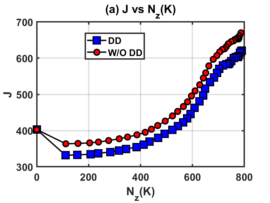
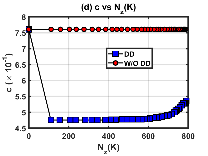
Figure 3: Case B (a), (b), (c), (d) show JJ, SBWS_{\text{BW}}, τo\tau_{o} and cc vs Nz​(𝐊)N_{z}(\mathbf{K}) where NzN_{z} is the number of zero elements of 𝐊\mathbf{K}. ‘DD’ and ‘W/O DD’ indicate Algorithm 1 and constant-delay algorithm respectively.

5.2 Delay-Design with Bandwidth Constraints

We next validate Algorithm 1. To illustrate its benefits, we compare it to an algorithm that consists of only the inner ADMM loop, referred to as the constant-delay algorithm. Both algorithms start from (𝐊∗,τo∗,τd∗)∈𝕂(\mathbf{K}^{*},\tau^{*}_{o},\tau^{*}_{d})\in\mathbb{K}. The delays τo∗\tau^{*}_{o} and τd∗\tau^{*}_{d} are kept constant throughout the constant-delay algorithm. In Case B, we present the simulations for a randomly generated LTI model 𝐀∈ℝ30×30{\mathbf{A}}\in\mathbb{R}^{30\times 30} and 𝐁=𝐁w=𝐐=𝐑=𝐈n\mathbf{B}=\mathbf{B}_{w}=\mathbf{Q}=\mathbf{R}=\mathbf{I}_{n}. We denote the number of zero elements of 𝐊\mathbf{K} by Nz​(𝐊)N_{z}(\mathbf{K}).

Case B: We consider a randomly generated 𝐀∈ℝ30×30\mathbf{A}\in\mathbb{R}^{30\times 30} with 900900 links in the cyber-layer, (c∗,τo∗)=(0.76,0.021)(c^{*},\tau^{*}_{o})=(0.76,0.021), mc​p=84m_{cp}=84 and mc​cm_{cc} =81=81. The initial conditions result in cm​i​n=0.475>c∗c_{min}=0.475>c^{*} from (32). However, (𝐊∗,cm​i​n)(\mathbf{K}^{*},c_{min}) is an unstable tuple, and therefore, we rely on O2.2 to co-design (𝐊,c)(\mathbf{K},c). Fig. 3 (a), (c) and (d) show that as sparsity increases, Algorithm 1 initially increases τo\tau_{o} and maintains cc to maintain optimality of JJ. As shown in Proposition 1, an increase in τo\tau_{o} decreases the bandwidth cost SBWS_{\text{BW}}. Moreover, since cc moves towards cm​i​nc_{min}, SBWS_{\text{BW}} decreases steeply for Algorithm 1. Further increase in sparsity of 𝐊\mathbf{K} causes the algorithm to decrease τo\tau_{o} and increase cc, which slows down the rate of decrease of SBWS_{\text{BW}} with respect to Nz​(𝐊)N_{z}(\mathbf{K}). Fig. 3 (a), (b) show that as a trade-off for a much lower SBWS_{\text{BW}} from Algorithm 1, we obtain JJ that is comparable to the constant-delay algorithm for all the sparsity levels.

6 Redesigning the CPS topology

Recall that the total system cost SS is composed of the bandwidth cost SBWS_{\text{BW}}, and the CN cost SCNS_{\text{CN}}. In Sec. 4, we designed an ℋ2\mathcal{H}_{2} optimal combination of sparse 𝐊\mathbf{K} and the delays τd\tau_{d} and τc\tau_{c} (i.e., bandwidths bc​pb_{cp} and bc​cb_{cc}) to decrease SBWS_{\text{BW}} while keeping SCNS_{\text{CN}} constant (i.e., keeping the topology 𝐓\mathbf{T} constant). In this section, as an additional step to Algorithm 1, we aim to further reduce the closed-loop ℋ2\mathcal{H}_{2} norm of the system by redesigning the CPS topology parameters 𝖃\boldsymbol{\mathfrak{X}}, 𝖓\boldsymbol{\mathfrak{n}}, 𝖀\boldsymbol{\mathfrak{U}} and 𝖒\boldsymbol{\mathfrak{m}} while keeping the gain matrix fixed at the sparse solution 𝐊\mathbf{K} of Algorithm 1. This redesign changes SCNS_{\text{CN}}, τd\tau_{d}, and τc\tau_{c}, which in turn changes the ℋ2\mathcal{H}_{2} norm JJ. In this process, SBWS_{\text{BW}} remains constant (i.e., the bandwidths remain fixed to the solution of Algorithm 1). Since an optimal redesign of the topology should decrease both SCNS_{\text{CN}} and JJ beyond the solution of Algorithm 1, we provide results on the existence of such an optimal topology and present a set of algorithms to obtain it.

6.1 Effect of Topology Variation on the CPS Parameters

Consider the system (5), which is implemented as a CPS following A.1-A.4. Before stating our design objective, we first discuss the effect of redesigning 𝐓\mathbf{T} with fixed 𝐊\mathbf{K}, bc​cb_{cc} and bc​pb_{cp} on the following CPS parameters.

6.1.1 Effect on the number of Communication Links

Recall from Sec. 2.2.1 and 2.2.2 that the number of inter-layer links is dependent on 𝐊\mathbf{K}, while the total number of intra-layer links are dependent on both 𝐊\mathbf{K} and 𝐓\mathbf{T}. Specifically, a non-zero i,ji,j-th off-diagonal block of the matrix 𝓚⁡(𝐊,𝐓)\boldsymbol{\mathcal{K}}(\mathbf{K},\mathbf{T}), defined in Sec. 2.2.1, represents an intra-layer link transmitting the nin_{i} states of CN ii to CN jj.

Refer to caption
Refer to caption
Figure 4: A simple diagram that depicts the change in CPS topology of Fig. 1 that occurs due to row and column permutations of 𝐊\mathbf{K}; See Example 2. Their are 99 intra-layer links in this topology compared to 1414 in Fig. 1 even though the nnz​(𝐊)\texttt{nnz}(\mathbf{K}) remains the same.
Example 2

Let us recall Example 1. For the system in Fig. 1, there are a total of ∑inoffi=14\sum_{i}{n_{\text{off}}}_{i}=14 intra-layer links. If we change the topology to 𝐓≡(𝖃=(2,1,5,7,3,4,6)𝐶𝐿𝑂𝑆𝐸\mathbf{T}\equiv\Big(\boldsymbol{\mathfrak{X}}=(2,1,5,7,3,4,6), 𝖀=(2,1,5,4,3,6)\boldsymbol{\mathfrak{U}}=(2,1,5,4,3,6), 𝖓=[1,1,1,1,1,2]T\boldsymbol{\mathfrak{n}}=[1,1,1,1,1,2]^{T}, 𝖒=[1,1𝐶𝐿𝑂𝑆𝐸,\boldsymbol{\mathfrak{m}}=[1,1, 1,1,1,1]T)1,1,1,1]^{T}\Big), then, 𝓚⁡(𝐊,𝐓)\boldsymbol{\mathcal{K}}(\mathbf{K},\mathbf{T}) is obtained as:

u∖x2⏞𝖝31⏞𝖝25⏞𝖝37⏞𝖝43⏞𝖝5\BAmulticolumn​2​c​46⏞𝖝6𝖚1​{1eghf𝖚2​{2adbc𝖚3​{3poq𝖚4​{4nlm𝖚5​{5ijk𝖚6​{6rs.\begin{array}[]{cccccccc}{{}_{u}\mkern-1.0mu\setminus\mkern-1.0mu{}^{x}}&{\overbrace{2}^{\boldsymbol{\mathfrak{x}}_{3}}}&{\overbrace{1}^{\boldsymbol{\mathfrak{x}}_{2}}}&{\overbrace{5}^{\boldsymbol{\mathfrak{x}}_{3}}}&{\overbrace{7}^{\boldsymbol{\mathfrak{x}}_{4}}}&{\overbrace{3}^{\boldsymbol{\mathfrak{x}}_{5}}}&\BAmulticolumn{2}{c}{\overbrace{4\hskip 13.6572pt6}^{\boldsymbol{\mathfrak{x}}_{6}}}\\ \\ \boldsymbol{\mathfrak{u}}_{1}\ \begin{cases}1\end{cases}&e&&g&h&f&&\\ \cline{2-8}\cr\boldsymbol{\mathfrak{u}}_{2}\ \begin{cases}2\end{cases}&&a&&d&&b&c\\ \cline{2-8}\cr\boldsymbol{\mathfrak{u}}_{3}\ \begin{cases}3\end{cases}&&&p&&&o&q\\ \cline{2-8}\cr\boldsymbol{\mathfrak{u}}_{4}\ \begin{cases}4\end{cases}&&&&n&l&m&\\ \cline{2-8}\cr\boldsymbol{\mathfrak{u}}_{5}\ \begin{cases}5\end{cases}&&&&&i&j&k\\ \cline{2-8}\cr\boldsymbol{\mathfrak{u}}_{6}\ \begin{cases}6\end{cases}&&&&&&r&s\\ \end{array}. (43)

Here, 𝐧𝐨𝐟𝐟=[0,0,1,2,2,4]{\mathbf{n}_{\mathbf{off}}}=[0,0,1,2,2,4] and therefore, the number of intra-layer links decrease from 1414 links in Example 1 to ∑inoffi=9\sum_{i}{n_{\text{off}}}_{i}=9, even though 𝐊\mathbf{K} remains the same. This effect of topology redesign on the assignment of the inter-layer and intra-layer links is shown in Fig. 4. As seen from the figure, the reassignment changes the destinations of the inter-layer links as well as both source and destinations of the intra-layer links. It, however, preserves the number of inter-layer links.

6.1.2 Effect on the Delays

From (10) and (11), it follows that varying 𝐓\mathbf{T} for a fixed (𝐊CLOSE,(\mathbf{K}, OPENbc​c,bc​p)b_{cc},b_{cp}) leads to a variation in τc​t​r=κ⁡(𝖓TCLOSE\tau_{ctr}=\kappa({\boldsymbol{\mathfrak{n}}}^{T} OPEN(𝐓)​𝐧𝐨𝐟𝐟​(𝐊,𝐓))/bc​c(\mathbf{T}){\mathbf{n}_{\mathbf{off}}}(\mathbf{K},\mathbf{T}))/b_{cc} but τd​t​r=κ⁡(nrow​(𝐊)+ncolCLOSE\tau_{dtr}=\kappa({n_{\text{row}}}(\mathbf{K})+{n_{\text{col}}} OPEN(𝐊))(\mathbf{K})) /bc​p)/b_{cp}) is kept constant (since the number of zero rows and columns will remain constant for a given 𝐊\mathbf{K}). In Algorithm 1, as 𝐓\mathbf{T} was fixed, both τd​p​r\tau_{dpr} and τc​p​r\tau_{cpr} were constant. In the current problem, however, 𝐓\mathbf{T} is the design variable, as a result of which both of these propagation delays become variable. Furthermore, we can no longer assume the per-link propagation delays for τc\tau_{c} and τd\tau_{d} to be equal as the choice of the destinations for the links is also variable. Therefore, we consider the worst case propagation delay for both, and accordingly replace the design variables τc​p​r\tau_{cpr} and τd​p​r\tau_{dpr} with maxi⁡(τc​p​ri)\max_{i}({\tau_{cpr}}_{i}) and maxi⁡(τd​p​ri)\max_{i}({\tau_{dpr}}_{i}) respectively, where τc​p​ri{\tau_{cpr}}_{i} and τd​p​ri{\tau_{dpr}}_{i} are the propagation delays in the corresponding ii-th link. This will be shown shortly when we formulate our optimization problem for the redesign.

6.1.3 Effect on the CN cost

The CN cost SCNS_{\text{CN}} consists of two parts - the rent cost SCNrS_{\text{CN}_{r}} and the computation overhead cost SCNcS_{\text{CN}_{c}}.

Assumption 1

SCNrS_{\text{CN}_{r}} is a strictly increasing function of the number of CNs 𝒩\mathcal{N}. SCNcS_{\text{CN}_{c}} is a strictly increasing function of (ni+mi)(n_{i}+m_{i}) for each CN ii.

Following Assumption 1, we define the computation overhead cost as

SCNc​(𝐓):=∑i=1𝒩(ni+mi)2,S_{\text{CN}_{c}}(\mathbf{T}):=\sum_{i=1}^{\mathcal{N}}\ (n_{i}+m_{i})^{2}, (44)

and the rent cost as

SCNr​(𝐓):={SCNcmax​𝒳(𝒩)|𝒳(𝒩)​is the 𝒩-th order statistic of random samples 𝒳i∼U⁡(0,1), i∈ℕ𝒩m},\displaystyle S_{\text{CN}_{r}}(\mathbf{T}):=\{S_{\text{CN}_{c}}^{\max}\mathcal{X}_{(\mathcal{N})}|\mathcal{X}_{(\mathcal{N})}\ \text{is the $\mathcal{N}$-th order statistic of random samples $\mathcal{X}_{i}\sim U(0,1)$, $i\in\mathbb{N}_{\mathcal{N}_{m}}$}\}, (45)

where SCNcmaxS_{\text{CN}_{c}}^{\max} =(m+n−2)2+4=(m+n-2)^{2}+4 is the maximum computation overhead cost possible for a system with mm inputs and nn states.

Refer to caption
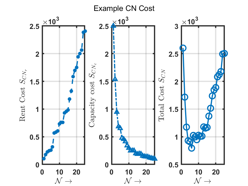
Figure 5: An example SCNS_{\text{CN}} vs 𝒩\mathcal{N} characteristics.

An example of total CN cost (SCNS_{\text{CN}}) vs. number of CNs (𝒩\mathcal{N}) for m=n=25m=n=25 is shown in Fig. 5. We can see that the SCNS_{\text{CN}} vs. 𝒩\mathcal{N} characteristics resemble a conventional marginal cost curve following the static pricing scheme used in cloud computing Aldossary et al., 2019. As the number of CNs reduces, SCNS_{\text{CN}} first decreases due to a decrease in SCNrS_{\text{CN}_{r}}. However, as 𝒩\mathcal{N} reduces further, the increase in SCNcS_{\text{CN}_{c}} overtakes the decrease in SCNrS_{\text{CN}_{r}}.

6.2 Design Objective

We next state our design objective as follows.

P2: Let the system (5) be implemented as a CPS following A.1-A.4 with maximum number of CNs 𝒩m=max⁡(m,n)\mathcal{N}_{m}=\max(m,n) CNs (Def. 1) and the initial topology denoted as 𝐓(i​n)|𝒩m\mathbf{T}^{(in)}|_{\mathcal{N}_{m}}. Let the outputs of Algorithm 1 when applied to this system be a sparse control gain matrix 𝐊∗\mathbf{K}^{*}, bandwidths bc​c∗b_{cc}^{*} and bc​p∗b_{cp}^{*}, and ℋ2\mathcal{H}_{2} norm J⁡(𝐊∗𝐶𝐿𝑂𝑆𝐸J(\mathbf{K}^{*}, 𝑂𝑃𝐸𝑁𝐓(i​n)|𝒩m)\mathbf{T}^{(in)}|_{\mathcal{N}_{m}}) 44 4 Since both τd\tau_{d} and τc\tau_{c} are functions of 𝐓\mathbf{T}, with a slight abuse of notation, we write J⁡(𝐊,𝐓)J(\mathbf{K},\mathbf{T}) in this section.. Then, assigning (𝐊,bc​c,bc​p)(\mathbf{K},b_{cc},b_{cp}) ≡\equiv (𝐊∗|𝒩m,bc​c∗|𝒩m,bc​p∗|𝒩m)(\mathbf{K}^{*}|_{\mathcal{N}_{m}},b^{*}_{cc}|_{\mathcal{N}_{m}},b^{*}_{cp}|_{\mathcal{N}_{m}}), find the optimal number of CNs 𝒩∗∈[2,𝒩m]\mathcal{N}^{*}\in[2,\mathcal{N}_{m}] and the corresponding optimal topology 𝐓∗|𝒩∗\mathbf{T}^{*}|_{\mathcal{N}^{*}} such that

  1. P2.1

    the closed-loop ℋ2\mathcal{H}_{2} norm is minimized and,

  2. P2.2

    the corresponding CN cost SCN​(𝐓∗|𝒩∗)S_{\text{CN}}(\mathbf{T}^{*}|_{\mathcal{N}^{*}}) ≤\leq SCNS_{\text{CN}} (𝐓(i​n)CLOSE(\mathbf{T}^{(in)} |𝒩m)|_{\mathcal{N}_{m}}), i.e., it remains at most the same as the CN cost for the initial topology.

The rationale behind the formulation of P2 is as follows. For a given topology 𝐓\mathbf{T}, there is a higher loss in the closed-loop ℋ2\mathcal{H}_{2} norm of (5) when block-wise sparsity is promoted in 𝐊\mathbf{K} compared to when the element-wise sparsity is promoted (Algorithm 1), assuming the same nnz​(𝐊)\texttt{nnz}(\mathbf{K}) in both the cases. However, block-wise sparsity in 𝐊\mathbf{K} is required to reduce the number of intra-layer links. Therefore, P1 focuses on promoting element-wise sparsity in 𝐊\mathbf{K}, and P2 rearranges its zero entries such that a block-wise sparse structure can be obtained. When combined with the variation in 𝐓\mathbf{T} to change the delays, this approach enables us to reduce JJ further than that obtained from Algorithm 1. We illustrate this approach in more detail in the simulation example in Sec. 7.2.

6.3 Algorithm Development

For a fixed 𝐊∗\mathbf{K}^{*}, each topology 𝐓|𝒩\mathbf{T}|_{\mathcal{N}} of the CPS (Def. 1) corresponds to an 𝒩×𝒩\mathcal{N}\times\mathcal{N} block matrix 𝓚|𝒩\boldsymbol{\mathcal{K}}|_{\mathcal{N}} through a bijective function 𝕶:(𝐊∗,𝐓|𝒩)→𝓚|𝒩\boldsymbol{\mathfrak{K}}:(\mathbf{K}^{*},\mathbf{T}|_{\mathcal{N}})\to\boldsymbol{\mathcal{K}}|_{\mathcal{N}} defined next. Let permutation matrices 𝐔∈ℝm×m\mathbf{U}\in\mathbb{R}^{m\times m} and 𝐗∈ℝn×n\mathbf{X}\in\mathbb{R}^{n\times n} be defined for a given 𝐓|𝒩=(𝖃|𝒩CLOSE\mathbf{T}|_{\mathcal{N}}=(\boldsymbol{\mathfrak{X}}|_{\mathcal{N}}, 𝖀|𝒩\boldsymbol{\mathfrak{U}}|_{\mathcal{N}}, 𝖓|𝒩\boldsymbol{\mathfrak{n}}|_{\mathcal{N}}, OPEN𝖒|𝒩)\boldsymbol{\mathfrak{m}}|_{\mathcal{N}}) as

𝐔\displaystyle\mathbf{U} :={𝐈m: permuted as ​(1,2,…,m)→𝖀},\displaystyle:=\{\mathbf{I}_{m}:\text{ permuted as }(1,2,\ldots,m)\to\boldsymbol{\mathfrak{U}}\}, (46)
𝐗\displaystyle\mathbf{X} :={𝐈n: permuted as ​(1,2,…,n)→𝖃}.\displaystyle:=\{\mathbf{I}_{n}:\text{ permuted as }(1,2,\ldots,n)\to\boldsymbol{\mathfrak{X}}\}. (47)

Then, the corresponding 𝓚|𝒩\boldsymbol{\mathcal{K}}|_{\mathcal{N}} is obtained as:

𝓚|𝒩=𝕶⁡(𝐊∗,𝐓|𝒩)=[𝐔𝐊∗​𝐗][𝖓|𝒩,𝖒|𝒩].\displaystyle\boldsymbol{\mathcal{K}}|_{\mathcal{N}}=\boldsymbol{\mathfrak{K}}(\mathbf{K}^{*},\mathbf{T}|_{\mathcal{N}})=[\mathbf{U}\mathbf{K}^{*}\mathbf{X}]_{[\boldsymbol{\mathfrak{n}}|_{\mathcal{N}},\boldsymbol{\mathfrak{m}}|_{\mathcal{N}}]}. (48)

Here, [𝐗][𝐚,𝐛][\mathbf{X}]_{[\mathbf{a},\mathbf{b}]} represents the partitioning of 𝐗\mathbf{X} using rowgroups 𝐚\mathbf{a} and colgroups 𝐛\mathbf{b} (see Example 1). Since 𝕶\boldsymbol{\mathfrak{K}} is invertible, the set of block matrices 𝓚|𝒩\boldsymbol{\mathcal{K}}|_{\mathcal{N}} that each correspond to a valid topology for 𝒩\mathcal{N} CNs can be written as:

{𝓚|𝒩}:={𝓚|𝒩:𝐓|𝒩=𝕶−1​(𝐊∗,𝓚|𝒩)​ defines a topology from Def. 1 }.\displaystyle\{\boldsymbol{\mathcal{K}}|_{\mathcal{N}}\}:=\{\boldsymbol{\mathcal{K}}|_{\mathcal{N}}:\mathbf{T}|_{\mathcal{N}}=\boldsymbol{\mathfrak{K}}^{-1}(\mathbf{K}^{*},\boldsymbol{\mathcal{K}}|_{\mathcal{N}})\text{ defines a topology from Def. \ref{def:topology} }\}. (49)

To solve P2, we first choose optimal 𝓚∗|2\boldsymbol{\mathcal{K}}^{*}|_{2}, ⋯\cdots, 𝓚∗|𝒩m\boldsymbol{\mathcal{K}}^{*}|_{\mathcal{N}_{m}} from the sets {𝓚|2}\{\boldsymbol{\mathcal{K}}|_{2}\}, ⋯\cdots, {𝓚|𝒩m}\{\boldsymbol{\mathcal{K}}|_{\mathcal{N}_{m}}\} such that their corresponding CN costs fulfill P2.2; the guidelines for this choice will be defined shortly. Out of these 𝒩m−1\mathcal{N}_{m}-1 matrices, we choose 𝓚∗|𝒩∗\boldsymbol{\mathcal{K}}^{*}|_{\mathcal{N}^{*}} as the one that corresponds to the minimum closed-loop ℋ2\mathcal{H}_{2} norm. The solution of P2 will then be obtained as 𝐓∗|𝒩∗\mathbf{T}^{*}|_{\mathcal{N}^{*}} == 𝕶−1​(𝐊∗,𝓚∗|𝒩∗)\boldsymbol{\mathfrak{K}}^{-1}(\mathbf{K}^{*},\boldsymbol{\mathcal{K}}^{*}|_{\mathcal{N}^{*}}). We begin with the steps for obtaining {𝓚|𝒩}\{\boldsymbol{\mathcal{K}}|_{\mathcal{N}}\} in (49) for 𝒩=2\mathcal{N}=2.

6.3.1 Block Diagonal Permutation

To obtain 𝓚∗|𝒩=2\boldsymbol{\mathcal{K}}^{*}|_{\mathcal{N}=2}, we first need to find 𝐔\mathbf{U} and 𝐗\mathbf{X} such that the majority of the zeros in 𝐊∗\mathbf{K}^{*} are delegated to the off-diagonal blocks 𝓚1,2\boldsymbol{\mathcal{K}}_{1,2} and 𝓚2,1\boldsymbol{\mathcal{K}}_{2,1}.

𝓚|2=[𝐔𝐊∗​𝐗][𝖓|2,𝖒|2]=[𝓚1,1𝓚1,2𝓚2,1𝓚2,2].\boldsymbol{\mathcal{K}}|_{2}=[\mathbf{U}\mathbf{K}^{*}\mathbf{X}]_{[\boldsymbol{\mathfrak{n}}|_{2},\boldsymbol{\mathfrak{m}}|_{2}]}=\begin{bmatrix}\boldsymbol{\mathcal{K}}_{1,1}&\boldsymbol{\mathcal{K}}_{1,2}\\ \boldsymbol{\mathcal{K}}_{2,1}&\boldsymbol{\mathcal{K}}_{2,2}\end{bmatrix}. (50)

This is done so that the total number of non-zero off-diagonal blocks ∑𝐧𝐨𝐟𝐟​(𝓚|𝒩=2)\sum{\mathbf{n}_{\mathbf{off}}}(\boldsymbol{\mathcal{K}}|_{\mathcal{N}=2}), i.e., the number of intra-layer links decreases. For a fixed bc​c∗b^{*}_{cc}, this can result in a decrease in the intra-layer transmission delay τc​t​r\tau_{ctr} and eventually in the closed-loop ℋ2\mathcal{H}_{2} norm.

We use the spectral partitioning method based on the Fiedler vector to carry out the block diagonal permutations, following its variant for rectangular matrices as presented in Kolda, 1998. Algorithm 2a states the steps for carrying out these permutations. Since the block sizes, i.e., 𝖓|2\boldsymbol{\mathfrak{n}}|_{2} and 𝖒|2\boldsymbol{\mathfrak{m}}|_{2} are unknown, we assign m1=floor​[m/2]m_{1}=\texttt{floor}[m/2] and n1=floor​[n/2]n_{1}=\texttt{floor}[n/2] to avoid a trivial solution. The actual block sizes are determined after obtaining 𝐔𝐊∗​𝐗\mathbf{U}\mathbf{K}^{*}\mathbf{X}, as seen next.

6.3.2 Optimal Partitioning

Once 𝐔\mathbf{U} and 𝐗\mathbf{X} are obtained from Algorithm 2a, we next search for sets of 𝖓|2\boldsymbol{\mathfrak{n}}|_{2} and 𝖒|2\boldsymbol{\mathfrak{m}}|_{2} to obtain the feasible set {𝓚|2}\{\boldsymbol{\mathcal{K}}|_{2}\}. There are (m−1)×(n−1)(m-1)\times(n-1) ways to partition 𝐔𝐊∗​𝐗\mathbf{U}\mathbf{K}^{*}\mathbf{X} as a 2×22\times 2 block matrix. For example, if m=n=3m=n=3, then 𝓚\boldsymbol{\mathcal{K}} could be partitioned into a 2×22\times 2 block matrix in the following 44 ways:

[∙⯀∙∙✶▴▴∙◆][∙⯀∙∙✶▴▴∙◆][∙⯀∙∙✶▴▴∙◆][∙⯀∙∙✶▴▴∙◆]𝖓|2[1,2][1,2][2,1][2,1]𝖒|2[1,2][2,1][1,2][2,1]\displaystyle\begin{array}[]{cccccc}&\left[\begin{array}[]{c|cc}\bullet&\sqbullet&\bullet\\ \hline\cr\bullet&\varstar&\blacktriangleup\\ \blacktriangleup&\bullet&\blackdiamond\end{array}\right]&\left[\begin{array}[]{c|cc}\bullet&\sqbullet&\bullet\\ \bullet&\varstar&\blacktriangleup\\ \hline\cr\blacktriangleup&\bullet&\blackdiamond\end{array}\right]&\left[\begin{array}[]{cc|c}\bullet&\sqbullet&\bullet\\ \hline\cr\bullet&\varstar&\blacktriangleup\\ \blacktriangleup&\bullet&\blackdiamond\end{array}\right]&\left[\begin{array}[]{cc|c}\bullet&\sqbullet&\bullet\\ \bullet&\varstar&\blacktriangleup\\ \hline\cr\blacktriangleup&\bullet&\blackdiamond\end{array}\right]\\[28.45274pt] \boldsymbol{\mathfrak{n}}|_{2}&[1,2]&[1,2]&[2,1]&[2,1]\\[14.22636pt] \boldsymbol{\mathfrak{m}}|_{2}&[1,2]&[2,1]&[1,2]&[2,1]\end{array}
Algorithm 2a Spectral Partitioning Algorithm
1: Input: Sparse matrix 𝐊∗∈ℝm×n\mathbf{K}^{*}\in\mathbb{R}^{m\times n}
2: Symmetrize 𝐊∗\mathbf{K}^{*} as 𝐊^∗=[𝟎​𝐊∗;𝐊∗T​ 0]\hat{\mathbf{K}}^{*}=[\mathbf{0}\ \mathbf{K}^{*};{\mathbf{K}^{*}}^{T}\ \mathbf{0}]
3: Compute Laplacian of 𝐊^∗\hat{\mathbf{K}}^{*} : 𝐋=𝐃−𝐊^∗\mathbf{L}=\mathbf{D}-\hat{\mathbf{K}}^{*}, where 𝐃=Diag​{d1,d2,…,dm+n}\mathbf{D}=\texttt{Diag}\{d_{1},d_{2},\ldots,d_{m+n}\} and di=∑j𝐊^i​j∗d_{i}=\sum_{j}\hat{\mathbf{K}}^{*}_{ij}
4: Find w as the eigenvector corresponding to the smallest positive eigenvalue of 𝐋\mathbf{L} or Fiedler vector
5: wf∈ℝm\texttt{w}_{f}\in\mathbb{R}^{m} and wl∈ℝn\texttt{w}_{l}\in\mathbb{R}^{n} denote first mm and last nn elements of w, respectively.
6: Sort wf\texttt{w}_{f} and wl\texttt{w}_{l} in descending order and denote the corresponding sorted indices as {i1,i2,…,im}\{i_{1},i_{2},\ldots,i_{m}\} and {j1,j2,…,jn}\{j_{1},j_{2},\ldots,j_{n}\}.
7: 𝐔:=𝐈m with rows permuted as {i1,i2,…,im} \mathbf{U}:=\text{$\mathbf{I}_{m}$ with rows permuted as $\{i_{1},i_{2},\ldots,i_{m}\}$ }
8: 𝐗:=𝐈n with rows permuted as {j1,j2,…,jm} \mathbf{X}:=\text{$\mathbf{I}_{n}$ with rows permuted as $\{j_{1},j_{2},\ldots,j_{m}\}$ }
9: Result: Permutation matrices 𝐔\mathbf{U}, 𝐗\mathbf{X}, rowgroup 𝖀={i1,i2,…,im}\boldsymbol{\mathfrak{U}}=\{i_{1},i_{2},\ldots,i_{m}\} and colgroup 𝖃={j1,j2,…,jm}\boldsymbol{\mathfrak{X}}=\{j_{1},j_{2},\ldots,j_{m}\}
Algorithm 2b Optimal Partitioning Algorithm
1: Input: Initial sparse gain matrix 𝐊∗\mathbf{K}^{*}, CN Cost SCN​(𝐓(i​n)|𝒩m)S_{\text{CN}}(\mathbf{T}^{(in)}|_{\mathcal{N}_{m}}), ℋ2\mathcal{H}_{2} norm J⁡(𝐊∗,𝐓(i​n)|𝒩m)J(\mathbf{K}^{*},\mathbf{T}^{(in)}|_{\mathcal{N}_{m}})
2: Input: [𝐔𝐊∗​𝐗][\mathbf{U}\mathbf{K^{*}}\mathbf{X}], 𝖀\boldsymbol{\mathfrak{U}} and 𝖃\boldsymbol{\mathfrak{X}} from Algorithm 2a
3: for i=1i=1 till m−1m-1 do
4:   Set 𝖒=[i,m−i]T\boldsymbol{\mathfrak{m}}=[i,m-i]^{T}
5:   for j=1j=1 till n−1n-1 do
6:    Set 𝖓=[j,n−j]T\boldsymbol{\mathfrak{n}}=[j,n-j]^{T}
7:    Set 𝐓:=(𝖃,𝖀,𝖓,𝖒)\mathbf{T}:=(\boldsymbol{\mathfrak{X}},\boldsymbol{\mathfrak{U}},\boldsymbol{\mathfrak{n}},\boldsymbol{\mathfrak{m}}) for current iteration
8:    Calculate τc​(𝐓)\tau_{c}(\mathbf{T}), τd​(𝐓)\tau_{d}(\mathbf{T}) and SC​N​(𝐓)S_{CN}(\mathbf{T})
9:    Calculate J⁡(𝐊∗,τc,τd)J(\mathbf{K}^{*},\tau_{c},\tau_{d}) for the current iter
10:     -ation’s 𝖒\boldsymbol{\mathfrak{m}} and 𝖓\boldsymbol{\mathfrak{n}}   
11: Choose the partitionings 𝖒\boldsymbol{\mathfrak{m}}, 𝖓\boldsymbol{\mathfrak{n}} for which the corresponding SC​N​(𝐓)S_{CN}(\mathbf{T}) ≤\leq SC​N​(𝐓(i​n)|𝒩m)S_{CN}(\mathbf{T}^{(in)}|_{\mathcal{N}_{m}})
12: Out of the remaining partitionings, choose the one that corresponds to the lowest ℋ2\mathcal{H}_{2} norm and set 𝐓∗|𝒩=𝐓\mathbf{T}^{*}|_{\mathcal{N}}=\mathbf{T} for that partitioning
13: Result: Topology 𝐓∗|𝒩\mathbf{T}^{*}|_{\mathcal{N}} for 𝒩\mathcal{N} number of CNs

The computation of {𝓚|2}\{\boldsymbol{\mathcal{K}}|_{2}\} is detailed in Algorithm 2b. We next discuss the variation of τc\tau_{c}, τd\tau_{d}, SCNS_{\text{CN}} over the set {𝓚|𝒩}\{\boldsymbol{\mathcal{K}}|_{\mathcal{N}}\}.

∙\bullet τd​(𝓚|𝒩)\tau_{d}(\boldsymbol{\mathcal{K}}|_{\mathcal{N}}): While τd​t​r​(𝐊∗)\tau_{dtr}(\mathbf{K}^{*}) remains constant, τd​p​r​(𝐓CLOSE\tau_{dpr}(\mathbf{T} |𝒩)|_{\mathcal{N}}) ≡τd​p​r​(𝕶−1​(𝐊∗,𝓚|𝒩))\equiv\tau_{dpr}(\boldsymbol{\mathfrak{K}}^{-1}(\mathbf{K}^{*},\boldsymbol{\mathcal{K}}|_{\mathcal{N}}))55 5 Here, 𝕶−1​(𝐊∗,𝓚|𝒩)\boldsymbol{\mathfrak{K}}^{-1}(\mathbf{K}^{*},\boldsymbol{\mathcal{K}}|_{\mathcal{N}}) is the inverse of the function 𝕶⁡(𝐊∗CLOSE\boldsymbol{\mathfrak{K}}(\mathbf{K}^{*} OPEN𝐓|𝒩)\mathbf{T}|_{\mathcal{N}}) in the argument 𝐓|𝒩\mathbf{T}|_{\mathcal{N}} for fixed 𝐊∗\mathbf{K}^{*}, as given in (48). varies over {𝓚|𝒩}\{\boldsymbol{\mathcal{K}}|_{\mathcal{N}}\}.

∙\bullet τc​(𝓚|𝒩)\tau_{c}(\boldsymbol{\mathcal{K}}|_{\mathcal{N}}): Both τc​t​r\tau_{ctr} and τc​p​r\tau_{cpr} are functions of 𝐓\mathbf{T} and therefore, can vary over {𝓚|𝒩}\{\boldsymbol{\mathcal{K}}|_{\mathcal{N}}\}. To ensure that τc​p​r\tau_{cpr} remains constant or decreases over {𝓚|𝒩}\{\boldsymbol{\mathcal{K}}|_{\mathcal{N}}\} for 𝒩<𝒩m\mathcal{N}<\mathcal{N}_{m}, we can choose an 𝒩\mathcal{N}-dimensional set of CNs (out of 𝒩m\mathcal{N}_{m}). We formally state the existence of such a set in the following lemma.

Lemma 3

Assume a CPS with parameters (𝐊∗𝐶𝐿𝑂𝑆𝐸(\mathbf{K}^{*}, bc​c∗b^{*}_{cc}, 𝑂𝑃𝐸𝑁𝒩m)\mathcal{N}_{m}) and topology 𝐓(i​n)|𝒩m\mathbf{T}^{(in)}|_{\mathcal{N}_{m}} that results in the intra-layer propagation delay τc​p​r​(𝐓(i​n)|𝒩m)\tau_{cpr}(\mathbf{T}^{(in)}|_{\mathcal{N}_{m}}). For any 𝒩≤𝒩m\mathcal{N}\leq\mathcal{N}_{m}, one can always choose an 𝒩\mathcal{N}-dimensional set of CNs such that for all topologies 𝐓|𝒩\mathbf{T}|_{\mathcal{N}}, τc​p​r​(𝐓|𝒩)≤τc​p​r​(𝐓(i​n)|𝒩m)\tau_{cpr}(\mathbf{T}|_{\mathcal{N}})\leq\tau_{cpr}(\mathbf{T}^{(in)}|_{\mathcal{N}_{m}}). ■\blacksquare

∙\bullet SCN​(𝓚|𝒩)S_{\text{CN}}(\boldsymbol{\mathcal{K}}|_{\mathcal{N}}): Rent cost SCNrS_{\text{CN}_{r}} is constant but the computation overhead cost SCNc​(𝐓|𝒩)≡SCNcS_{\text{CN}_{c}}(\mathbf{T}|_{\mathcal{N}})\equiv S_{\text{CN}_{c}} (𝕶−1​(𝓚|𝒩))(\boldsymbol{\mathfrak{K}}^{-1}(\boldsymbol{\mathcal{K}}|_{\mathcal{N}}))5 varies over {𝓚|𝒩}\{\boldsymbol{\mathcal{K}}|_{\mathcal{N}}\}.

Our objective is to find the optimal 𝓚∗|𝒩\boldsymbol{\mathcal{K}}^{*}|_{\mathcal{N}} out of {𝓚|𝒩}\{\boldsymbol{\mathcal{K}}|_{\mathcal{N}}\} that minimizes the closed-loop ℋ2\mathcal{H}_{2} norm under the constraint that the CN cost does not increase from that in Algorithm 1.

O3:𝓚∗|𝒩=\displaystyle\textbf{O3:}\ \boldsymbol{\mathcal{K}}^{*}|_{\mathcal{N}}=\ argmin{𝓚|𝒩}​J​(τc​(𝓚|𝒩),τd​(𝐓⁡(𝓚|𝒩)),𝐊∗),\displaystyle\underset{\{\boldsymbol{\mathcal{K}}|_{\mathcal{N}}\}}{\text{argmin}}\ J(\tau_{c}(\boldsymbol{\mathcal{K}}|_{\mathcal{N}}),\tau_{d}(\mathbf{T}(\boldsymbol{\mathcal{K}}|_{\mathcal{N}})),\mathbf{K}^{*}), (65)
s.t.SCN​(𝓚|𝒩)≤SCN​(𝐓(i​n)|𝒩m).\displaystyle\text{s.t.}\ \ \ S_{\text{CN}}(\boldsymbol{\mathcal{K}}|_{\mathcal{N}})\leq S_{\text{CN}}(\mathbf{T}^{(in)}|_{\mathcal{N}_{m}}). (66)

Algorithm 2 obtains 𝐓∗|2≡𝕶−1​(𝐊∗,𝓚∗|2)\mathbf{T}^{*}|_{{2}}\equiv\boldsymbol{\mathfrak{K}}^{-1}(\mathbf{K}^{*},\boldsymbol{\mathcal{K}}^{*}|_{2})5 by solving O3. This is the optimal topology that can be implemented for a 22 CN CPS. To obtain the same for 𝒩>2\mathcal{N}>2 CNs, the diagonal blocks of 𝓚|2\boldsymbol{\mathcal{K}}|_{2} are further divided into their constituent 2×22\times 2 blocks recursively by using Algorithm 2. Once all the diagonal blocks are exhausted, i.e., cannot be further divided, the off-diagonals blocks follow the same recursive division process, until we obtain 𝐓∗|𝒩m≡𝕶−1​(𝓚∗|𝒩m)\mathbf{T}^{*}|_{\mathcal{N}_{m}}\equiv\boldsymbol{\mathfrak{K}}^{-1}(\boldsymbol{\mathcal{K}}^{*}|_{\mathcal{N}_{m}}). Finally, the optimal topology from the designed 𝐓∗|2\mathbf{T}^{*}|_{2}, 𝐓∗|3\mathbf{T}^{*}|_{3}, ⋯\cdots, 𝐓∗|𝒩m\mathbf{T}^{*}|_{\mathcal{N}_{m}} is chosen such that min𝒩⁡J⁡(𝐓∗|𝒩)\min_{\mathcal{N}}J(\mathbf{T}^{*}|_{\mathcal{N}}). The optimization O3 is trivially feasible for 𝒩m\mathcal{N}_{m} CNs. We next state the proposition that derives the conditions under which O3 is feasible for any 𝒩<𝒩m\mathcal{N}<\mathcal{N}_{m}.

Proposition 2

Assume a CPS with 𝒩m\mathcal{N}_{m} CNs and fixed (𝐊∗𝐶𝐿𝑂𝑆𝐸(\mathbf{K}^{*}, bc​c∗b^{*}_{cc}, 𝑂𝑃𝐸𝑁bc​p∗)b^{*}_{cp}) has a topology 𝐓(i​n)|𝒩m\mathbf{T}^{(in)}|_{\mathcal{N}_{m}}, intra-link transmission delay τc​t​r​(𝐓(i​n)|𝒩m)\tau_{ctr}(\mathbf{T}^{(in)}|_{\mathcal{N}_{m}}), and CN cost SCN​(𝐓(i​n)𝐶𝐿𝑂𝑆𝐸S_{\text{CN}}(\mathbf{T}^{(in)} |𝒩m)|_{\mathcal{N}_{m}}). Let Algorithm 2 be used to obtain a topology 𝐓∗|𝒩\mathbf{T}^{*}|_{\mathcal{N}} for 𝒩<𝒩m\mathcal{N}<\mathcal{N}_{m} such that the fraction of the total non-zero off-diagonal blocks in 𝓚⁡(𝐊∗,𝐓∗|𝒩)\boldsymbol{\mathcal{K}}(\mathbf{K}^{*},\mathbf{T}^{*}|_{\mathcal{N}}) is less than or equal to that in 𝓚⁡(𝐊∗,𝐓∗|𝒩m)\boldsymbol{\mathcal{K}}(\mathbf{K}^{*},\mathbf{T}^{*}|_{\mathcal{N}_{m}}), i.e.,

∑i𝒩noffi​(𝐊∗,𝐓∗|𝒩)𝒩⁡(𝒩−1)≤∑i𝒩mnoffi​(𝐊∗,𝐓(i​n)|𝒩m)𝒩m​(𝒩m−1).\frac{\sum_{i}^{\mathcal{N}}{n_{\text{off}}}_{i}(\mathbf{K}^{*},\mathbf{T}^{*}|_{\mathcal{N}})}{\mathcal{N}(\mathcal{N}-1)}\leq\frac{\sum_{i}^{\mathcal{N}_{m}}{n_{\text{off}}}_{i}(\mathbf{K}^{*},\mathbf{T}^{(in)}|_{\mathcal{N}_{m}})}{\mathcal{N}_{m}(\mathcal{N}_{m}-1)}. (67)

When n≤mn\leq m, there always exists an optimal number of CNs 𝒩∗<𝒩m\mathcal{N}^{*}<\mathcal{N}_{m} for which τc​t​r​(𝐓∗|𝒩∗)<τc​t​r​(𝐓(i​n)𝐶𝐿𝑂𝑆𝐸\tau_{ctr}(\mathbf{T}^{*}|_{\mathcal{N}^{*}})<\tau_{ctr}(\mathbf{T}^{(in)} |𝒩m)|_{\mathcal{N}_{m}}) and SCN​(𝐓∗|𝒩∗)S_{\text{CN}}(\mathbf{T}^{*}|_{\mathcal{N}^{*}}) ≤\leq SCN​(𝐓(i​n)|𝒩m)S_{\text{CN}}(\mathbf{T}^{(in)}|_{\mathcal{N}_{m}}). When n>mn>m. then this result holds if n≤12​m​(m−1)n\leq\frac{1}{2}m(m-1). ■\blacksquare

Lemma 3 and Proposition 2 provide sufficient conditions under which intra-layer delay τc​(𝐓∗|𝒩∗)\tau_{c}(\mathbf{T}^{*}|_{\mathcal{N}^{*}}) <τc​(𝐓(i​n)CLOSE<\tau_{c}(\mathbf{T}^{(in)} |𝒩m)|_{\mathcal{N}_{m}}) for some 𝒩∗\mathcal{N}^{*} <𝒩m<\mathcal{N}_{m}. If the increase in the corresponding τd​(𝐓∗|𝒩∗)\tau_{d}(\mathbf{T}^{*}|_{\mathcal{N}^{*}}) is limited such that (τc​(𝐓∗|𝒩∗)+τd​(𝐓∗|𝒩∗))(\tau_{c}(\mathbf{T}^{*}|_{\mathcal{N}^{*}})+\tau_{d}(\mathbf{T}^{*}|_{\mathcal{N}^{*}})) << (τc​(𝐓(i​n)|𝒩m)+τd​(𝐓(i​n)|𝒩m))(\tau_{c}(\mathbf{T}^{(in)}|_{\mathcal{N}_{m}})+\tau_{d}(\mathbf{T}^{(in)}|_{\mathcal{N}_{m}})), one can obtain J⁡(𝐓∗|𝒩∗)<J⁡(𝐓(i​n)|𝒩m)J(\mathbf{T}^{*}|_{\mathcal{N}^{*}})<J(\mathbf{T}^{(in)}|_{\mathcal{N}_{m}}). Otherwise, one should stick to the initial topology 𝐓(i​n)|𝒩m\mathbf{T}^{(in)}|_{\mathcal{N}_{m}}. Note that τc​p​r​(𝐓∗|𝒩∗)\tau_{cpr}(\mathbf{T}^{*}|_{\mathcal{N}^{*}}) may also be lesser than the initial value τc​p​r​(𝐓(i​n)|𝒩m)\tau_{cpr}(\mathbf{T}^{(in)}|_{\mathcal{N}_{m}}), as shown in Lemma 3. This can result in a further decrease in the overall delay τc​(𝐓∗|𝒩∗)+τd​(𝐓∗|𝒩∗)\tau_{c}(\mathbf{T}^{*}|_{\mathcal{N}^{*}})+\tau_{d}(\mathbf{T}^{*}|_{\mathcal{N}^{*}}).

Refer to caption
Refer to caption
Refer to caption

(a) 𝐓(i​n)|𝒩m=30\mathbf{T}^{(in)}|_{\mathcal{N}_{m}=30}           (b) 𝐓∗|𝒩=4\mathbf{T}^{*}|_{\mathcal{N}=4}              (c) 𝐓∗|𝒩=11\mathbf{T}^{*}|_{\mathcal{N}=11}

Refer to caption
Refer to caption
Refer to caption

(d) 𝐓∗|𝒩m=20\mathbf{T}^{*}|_{\mathcal{N}_{m}=20}            (e) 𝐓∗|𝒩=28\mathbf{T}^{*}|_{\mathcal{N}=28}              (f) 𝐓∗|𝒩=30\mathbf{T}^{*}|_{\mathcal{N}=30}

▴\blacktriangleup Actuator       ∙\bullet Sensor       ⯀\sqbullet CN       −⁣−-- Inter-layer link carrying 𝐮⁡(t)\mathbf{u}(t)

⋯\cdots Inter-layer link carrying 𝐱⁡(t)\mathbf{x}(t)     −⋅−-\cdot- Intra-layer link carrying 𝐱⁡(t)\mathbf{x}(t)

Figure 6: Case B: (a) shows the initial topology 𝐓(i​n)|𝒩m\mathbf{T}^{(in)}|_{\mathcal{N}_{m}} for 𝒩m=30\mathcal{N}_{m}=30 CNs used in Algorithm 1. The optimal topologies for 𝒩=4\mathcal{N}=4, 1111, 2020, 2828 and 3030 obtained from Algorithm 2 are shown in (b), (c), (d), (e) and (f) respectively.

7 Examples

We apply Algorithm 2 to the simulation example of Case B presented in Sec. 5. A sparse 𝐊∗\mathbf{K}^{*} obtained from Algorithm 1 with the corresponding topology 𝐓(i​n)|𝒩m=30\mathbf{T}^{(in)}|_{\mathcal{N}_{m}=30} is used as the input to Algorithm 2. The values of 𝖃(i​n)|30\boldsymbol{\mathfrak{X}}^{(in)}|_{30}, 𝖀(i​n)|30\boldsymbol{\mathfrak{U}}^{(in)}|_{30}, 𝖓(i​n)|30\boldsymbol{\mathfrak{n}}^{(in)}|_{30} and 𝖒(i​n)|30\boldsymbol{\mathfrak{m}}^{(in)}|_{30} for this initial topology are randomly chosen and given in negi (2021). Moreover, the values of τd​(𝐓(i​n)|30)\tau_{d}(\mathbf{T}^{(in)}|_{30}), τc​(𝐓(i​n)|30)\tau_{c}(\mathbf{T}^{(in)}|_{30}), SCN​(𝐓(i​n)|30)S_{\text{CN}}(\mathbf{T}^{(in)}|_{30}) and J⁡(𝐊∗CLOSE,J(\mathbf{K}^{*}, OPEN𝐓(i​n)|30)\mathbf{T}^{(in)}|_{30}) are used to normalize the corresponding τd​(𝐓∗|𝒩)\tau_{d}(\mathbf{T}^{*}|_{\mathcal{N}}), τc​(𝐓∗|𝒩)\tau_{c}(\mathbf{T}^{*}|_{\mathcal{N}}), SCN​(𝐓∗|𝒩)S_{\text{CN}}(\mathbf{T}^{*}|_{\mathcal{N}}) and J⁡(𝐊∗,𝐓∗|𝒩)J(\mathbf{K}^{*},\mathbf{T}^{*}|_{\mathcal{N}}) for optimal topologies 𝐓∗|𝒩\mathbf{T}^{*}|_{\mathcal{N}} obtained as the outputs of Algorithm 2. For e.g., a normalized τc​(𝐓∗|𝒩)=0.8\tau_{c}(\mathbf{T}^{*}|_{\mathcal{N}})=0.8 means that for some 𝒩<𝒩m\mathcal{N}<\mathcal{N}_{m}, Algorithm 2 obtains a topology with 20%20\% less intra-layer delay compared to the initial topology.

7.1 Applying Algorithm 2 to Case B

The input to Algorithm 2 is a sparse 𝐊∗∈ℝ30×30\mathbf{K}^{*}\in\mathbb{R}^{30\times 30} with nnz=131\texttt{nnz}=131. Fig. 6 (a) shows the initial topology 𝐓(i​n)|30\mathbf{T}^{(in)}|_{30}, while Fig. 6 (b) - (f) show the optimal topologies 𝐓∗|𝒩\mathbf{T}^{*}|_{\mathcal{N}} obtained as the output of Algorithm 2 for 𝒩=4\mathcal{N}=4, 1111, 2020, 2828 and 3030, respectively. In these figures, the size of the square representing a CN is directly proportional to the number of states and inputs associated with it. Thus, these figures show how Algorithm 2 modifies the number of states and inputs associated with each CN to satisfy O3 as 𝒩\mathcal{N} changes. Furthermore, they show the subset of 𝒩\mathcal{N} chosen out of 𝒩m\mathcal{N}_{m} CNs to fulfill Lemma 3. Fig. 7 shows that Algorithm 2 guarantees a lower value of the closed-loop ℋ2\mathcal{H}_{2} norm for all 𝒩≤𝒩m\mathcal{N}\leq\mathcal{N}_{m} compared to J⁡(𝐊∗,𝐓(i​n)|𝒩m)J(\mathbf{K}^{*},\mathbf{T}^{(in)}|_{\mathcal{N}_{m}}). For the optimal topologies, any potential increase in τd​p​r\tau_{dpr} is compensated by the decrease in τc​t​r\tau_{ctr}, as seen for 𝒩=24\mathcal{N}=24. The CN cost SCNS_{\text{CN}} decreases continuously from 𝒩=30\mathcal{N}=30 until 𝒩=15\mathcal{N}=15, after which it starts increasing again as the sharp rise in SCNcS_{\text{CN}_{c}} overshadows the decrease in the cost of renting a lower number of CNs. The main message conveyed by Fig. 7 is that if one desires the lowest JJ such that SCN≤SCN​(𝐓(i​n)|𝒩m)S_{\text{CN}}\leq S_{\text{CN}}(\mathbf{T}^{(in)}|_{\mathcal{N}_{m}}), then one can choose the optimal topology 𝐓∗|𝒩\mathbf{T}^{*}|_{\mathcal{N}} obtained for 𝒩=2\mathcal{N}=2; however, if the goal is to obtain the lowest SCNS_{\text{CN}} such that J≤J⁡(𝐓(i​n)|𝒩m)J\leq J(\mathbf{T}^{(in)}|_{\mathcal{N}_{m}}), then one must choose the optimal topology corresponding to 𝒩=4\mathcal{N}=4.

Refer to caption
Figure 7: Case B: Comparison of normalized JJ, SS, τd\tau_{d} and τo\tau_{o} between different designed topologies 𝐓∗|2\mathbf{T}^{*}|_{2}, 𝐓∗|3\mathbf{T}^{*}|_{3}, ⋯\cdots 𝐓∗|30\mathbf{T}^{*}|_{30}. The normalization is with respect to the corresponding parameter values of the initially given topology.

7.2 Algorithm 2 vs Block-Sparse Algorithm of Negi and Chakrabortty, 2020b

Note that our approach is to first promote element-wise sparsity in the initial 𝐊∗\mathbf{K}^{*} using Algorithm 1, and then divide it into 𝒩=2,3,…,\mathcal{N}=2,3,\ldots, 𝒩m\mathcal{N}_{m} blocks using Algorithm 2. If one wants to directly promote block-wise sparsity in 𝐊∗\mathbf{K}^{*} for any number of blocks 𝒩\mathcal{N}, then one needs to know the corresponding initial block-structure a priori. We can use the block-structure obtained from Algorithm 2 for each 𝒩\mathcal{N} as that initial given structure and use the algorithm proposed in our recent paper Negi and Chakrabortty, 2020b to carry out direct block-sparsity promotion in 𝐊∗\mathbf{K}^{*}. The corresponding SBWS_{\text{BW}}, SCNS_{\text{CN}} and JJ values obtained are compared with the output of Algorithm 2 in Fig. 8. While SBWS_{\text{BW}} is held constant in Algorithm 2 (since it is already optimized in Algorithm 1), the SBWS_{\text{BW}} for block-sparse algorithm increases steeply as 𝒩\mathcal{N} increases. On the other hand, SCNS_{\text{CN}} for a given 𝒩\mathcal{N} is the same for both the algorithms because of the same corresponding block-structures. However, the ℋ2\mathcal{H}_{2} norm obtained through Algorithm 2 in each case is lower than that obtained through direct block-sparsity promotion for all 𝒩\mathcal{N}. The reason is that the latter must collectively sparsify an entire block as a result of which the ℋ2\mathcal{H}_{2} norm becomes more conservative. Our element-wise sparsification approach in Algorithm 1 manages to avoid this conservatism.

Refer to caption
Figure 8: Comparison of SBWS_{\text{BW}}, SCNS_{\text{CN}} and JJ between Algorithm 2 output and direct block-sparsity promotion in 𝐊∗\mathbf{K}^{*} for Case B

8 Conclusion

This paper presented the co-design of network delays and sparse controller for LTI systems to improve their ℋ2\mathcal{H}_{2} performance. Bandwidth cost constraint is imposed to ensure finite bandwidth distribution among the communication links. The challenges of co-design borne out of implicit functional relationships between the delays, the sparse controller, and the ℋ2\mathcal{H}_{2}-norm are overcome by a hierarchical algorithm, where the inner loop and outer loop are based on ADMM and SDP relaxations, respectively. Additional algorithms are derived for carrying out structural modifications in the sparse controller to manipulate the number and computation overhead of CNs such that both the ℋ2\mathcal{H}_{2} norm and the price of renting the agents are further reduced, at the cost of foregoing privacy of information. Numerical simulations show the effectiveness of the designs and bring out interesting observations about the relationship between the delays, sparsity, and ℋ2\mathcal{H}_{2} performance of the closed-loop system.

Appendix

8.1 Proof of Lemma 1

The i​jij-th block of 𝐀~\tilde{\mathbf{A}} is given as:

𝐀~i​j={∑k=1,k≠jN1θj−θk​𝐈n,i∈ℕN−1,i=j1θj−θi​∏m=1,m≠j,iNθi−θmθj−θm​𝐈n,i∈ℕN−1,i≠j𝐀,i=N,j∈ℕN−1.\tilde{\mathbf{A}}_{ij}=\begin{cases}\sum\limits_{k=1,\ k\neq j}^{N}\frac{1}{\theta_{j}-\theta_{k}}\mathbf{I}_{n},\hskip 48.36958pti\in\mathbb{N}_{N-1},i=j\\ \frac{1}{\theta_{j}-\theta_{i}}\prod\limits_{m=1,\ m\neq j,i}^{N}\frac{\theta_{i}-\theta_{m}}{\theta_{j}-\theta_{m}}\mathbf{I}_{n},\ \ \ i\in\mathbb{N}_{N-1},\ i\neq j\\ \mathbf{A},\hskip 110.96556pti=N,j\in\mathbb{N}_{N-1}.\end{cases} (68)

Substituting (14) in (68), the diagonal and off-diagonal block matrices of the first N−1N-1 block rows are given by:

𝐀~i​i=1τo​∑k=1,k≠iNai​k​𝐈n,𝐀~j​i=aj​iτo​∏m=1,m≠j,iNaj​mai​m​𝐈n,\displaystyle\tilde{\mathbf{A}}_{ii}=\frac{1}{\tau_{o}}\sum\limits_{k=1,\ k\neq i}^{N}a_{ik}\mathbf{I}_{n},\ \tilde{\mathbf{A}}_{ji}=\frac{a_{ji}}{\tau_{o}}\prod\limits_{m=1,\ m\neq j,i}^{N}\frac{a_{jm}}{a_{im}}\mathbf{I}_{n}, (69a)
ai​k=−(sin⁡(OPEN(2​N−i−k)​π)2​(N−1))​sin⁡((k−i)​π2​(N−1)))−1,\displaystyle a_{ik}=-\left({\sin\left(\frac{(2N-i-k)\pi)}{2(N-1)}\right)\sin\left(\frac{(k-i)\pi}{2(N-1)}\right)}\right)^{-1}, (69b)

where i,j∈{1,…,N}i,j\in\{1,\ldots,N\}. Therefore, 𝚲\boldsymbol{\Lambda} can be written as:

𝚲i​j={𝐀~i​j,i=1,…,N−1,j=1,…,N,𝟎,i=N,j=1,…,N.\displaystyle\boldsymbol{\Lambda}_{ij}=\begin{cases}\tilde{\mathbf{A}}_{ij},\ \ \ \ \ i=1,\ldots,N-1,\ j=1,\ldots,N,\\ \mathbf{0},\ \ \ \ \ \ i=N,\ j=1,\ldots,N.\end{cases} (70)

The proof follows from (68), (69) and (70). ■\blacksquare

8.2 Proof of Lemma 2

From (15) and (16), 𝐍d\mathbf{N}_{d} can be written as:

𝐍d=[l1​(−τd),…,lN​(−τd)]T⊗𝐈n.\displaystyle\mathbf{N}_{d}=[l_{1}(-\tau_{d}),\ldots,l_{N}(-\tau_{d})]^{T}\otimes\mathbf{I}_{n}. (71)

Let ϑk=cos⁡((N−k−1)​πN−1)\vartheta_{k}=\cos\left(\frac{(N-k-1)\pi}{N-1}\right) for k={0,…,N−1}k=\{0,\ldots,N-1\}. Using (14), (15a) and c=τd/τoc=\nicefrac{{\tau_{d}}}{{\tau_{o}}} we can write

lj​(−τd)=∏m=1,m≠jN−c−0.5​(ϑm−1−1)0.5​(ϑj−1−ϑm−1).\displaystyle l_{j}(-\tau_{d})=\prod\limits_{m=1,\ m\neq j}^{N}\frac{-c-0.5(\vartheta_{m-1}-1)}{0.5(\vartheta_{j-1}-\vartheta_{m-1})}. (72)

Using (71) and (72), 𝐍d\mathbf{N}_{d} can be rewritten in the form of (23) where the jj-th row of 𝚪\boldsymbol{\Gamma} contains the coefficients of lj​(−τd)l_{j}(-\tau_{d}). From (72), lj​(−τd)l_{j}(-\tau_{d}) is a product of N−1N-1 affine terms in cc whose coefficients are only dependent on NN, and therefore, 𝚪\boldsymbol{\Gamma} is a constant for constant NN. ■\blacksquare

8.3 Proof of Theorem 1

The proof of uniqueness of solution of (19) and differentiability of 𝐏\mathbf{P} utilizes Lemma 1 and 2, and follows procedure similar to Theorem 2.1 and Lemma 3.1 in Rautert and Sachs, 1997, respectively. Specifically, 𝐏′(τo)∂τo\mathbf{P}^{{}^{\prime}}(\tau_{o})\partial\tau_{o}, 𝐏′(c)∂c\mathbf{P}^{{}^{\prime}}(c)\partial c and 𝐏′(𝐊)dK\mathbf{P}^{{}^{\prime}}(\mathbf{K})dK follow as solutions of the following Lyapunov equations:

𝐀c​lT𝐏′(τo)∂τo+𝐏′(τo)∂τo𝐀c​l=∂τoτo2(𝚲T𝐏+𝐏𝚲),\displaystyle\mathbf{A}_{cl}^{T}\ \mathbf{P}^{{}^{\prime}}(\tau_{o})\partial\tau_{o}+\mathbf{P}^{{}^{\prime}}(\tau_{o})\partial\tau_{o}\ \mathbf{A}_{cl}=\frac{\partial\tau_{o}}{\tau^{2}_{o}}(\boldsymbol{\Lambda}^{T}\mathbf{P}+\mathbf{P}\boldsymbol{\Lambda}), (73)
𝐀c​lT𝐏′(c)∂c+𝐏′(c)∂c𝐀c​l=𝐍∂d′c𝐊dT𝐆+𝐆T𝐊d∂cT𝐍dT′,\displaystyle\mathbf{A}_{cl}^{T}\ \mathbf{P}^{{}^{\prime}}(c)\partial c+\mathbf{P}^{{}^{\prime}}(c)\partial c\ \mathbf{A}_{cl}=\mathbf{N}{{}^{\prime}}_{d}\partial c\mathbf{K}^{T}_{d}\mathbf{G}+\mathbf{G}^{T}\mathbf{K}_{d}\partial c^{T}{\mathbf{N}^{T}_{d}}^{{}^{\prime}}, (74)
𝐀c​lT𝐏′(𝐊)∂𝐊+𝐏′(𝐊)∂𝐊𝐀c​l=−𝐙d−𝐙dT−𝐙o−𝐙oT,\displaystyle\mathbf{A}_{cl}^{T}\mathbf{P}^{{}^{\prime}}(\mathbf{K})\partial\mathbf{K}+\mathbf{P}^{{}^{\prime}}(\mathbf{K})\partial\mathbf{K}\ \mathbf{A}_{cl}=-\mathbf{Z}_{d}-\mathbf{Z}^{T}_{d}-\mathbf{Z}_{o}-\mathbf{Z}^{T}_{o}, (75)

where 𝐙d=𝐍dT​(∂𝐊∘𝓘d)​𝐆\mathbf{Z}_{d}=\mathbf{N}^{T}_{d}(\partial\mathbf{K}\circ\boldsymbol{\mathcal{I}}_{d})\mathbf{G} and 𝐙o\mathbf{Z}_{o} == 𝐍oT\mathbf{N}^{T}_{o} (∂𝐊CLOSE(\partial\mathbf{K} ∘\circ OPEN𝓘o)​𝐆\boldsymbol{\mathcal{I}}_{o})\mathbf{G}. The partial derivative of J⁡(𝐊)J(\mathbf{K}) is J′​(𝐊)​∂𝐊=Tr​(𝓑T​𝐏′CLOSEJ^{\prime}(\mathbf{K})\partial\mathbf{K}=\text{Tr}(\boldsymbol{\mathcal{B}}^{T}\mathbf{P}^{\prime} (𝐊)𝓑)=Tr(∇J(𝐊)T∂𝐊)(\mathbf{K})\boldsymbol{\mathcal{B}})=\text{Tr}(\nabla J(\mathbf{K})^{T}\partial\mathbf{K}), where ∂𝐊∈ℝm×n\partial\mathbf{K}\in\mathbb{R}^{m\times n}. Post-multiplying (75) with 𝐋\mathbf{L} and taking its trace, we obtain

Tr(∂𝐊T∇J(𝐊))=Tr(∂𝐊dT𝐆𝐋𝐍d+∂𝐊oT𝐆𝐋𝐍o),\displaystyle\text{Tr}(\partial\mathbf{K}^{T}\nabla J(\mathbf{K}))=\text{Tr}\big(\partial\mathbf{K}_{d}^{T}\mathbf{G}\mathbf{L}\mathbf{N}_{d}+\partial\mathbf{K}_{o}^{T}\mathbf{G}\mathbf{L}\mathbf{N}_{o}\big), (76)

where ∂𝐊d=∂𝐊∘𝓘d\partial\mathbf{K}_{d}=\partial\mathbf{K}\circ\boldsymbol{\mathcal{I}}_{d} and ∂𝐊o=∂𝐊∘𝓘o\partial\mathbf{K}_{o}=\partial\mathbf{K}\circ\boldsymbol{\mathcal{I}}_{o}. Using the property Tr​((𝐗∘𝐘)T​𝐙)=Tr​(𝐗T​(𝐘∘𝐙))\text{Tr}((\mathbf{X}\circ\mathbf{Y})^{T}\mathbf{Z})=\text{Tr}(\mathbf{X}^{T}(\mathbf{Y}\circ\mathbf{Z})) (Schott, 2016, Prob. 8.37), where 𝐗,𝐘,𝐙∈ℝm×n\mathbf{X},\mathbf{Y},\mathbf{Z}\in\mathbb{R}^{m\times n} in (76), we get (27). Using (73) and (74), and a similar procedure as above, we obtain

J′​(τo)=−1τo2​Tr​(𝚲T​𝐏𝐋+𝐋𝐏​𝚲),\displaystyle J^{\prime}(\tau_{o})=-\frac{1}{\tau_{o}^{2}}\text{Tr}(\boldsymbol{\Lambda}^{T}\mathbf{P}\mathbf{L}+\mathbf{L}\mathbf{P}\boldsymbol{\Lambda}), (77)
J′(c)=Tr(𝐍d′𝐊dT𝐆𝐋+𝐋𝐆T𝐊d𝐍d′T).\displaystyle J^{\prime}(c)=\text{Tr}(\mathbf{N}^{{}^{\prime}}_{d}\mathbf{K}_{d}^{T}\mathbf{G}\mathbf{L}+\mathbf{L}\mathbf{G}^{T}\mathbf{K}_{d}{\mathbf{N}^{{}^{\prime}}_{d}}^{T}). (78)

We can subsequently obtain (26) from (77) and (78). ■\blacksquare

8.4 Proof of Theorem 2

Using ϕ0\boldsymbol{\phi}_{0}, ϕ1\boldsymbol{\phi}_{1}, ψ0\psi_{0}, 𝐀1\mathbf{A}_{1} and Δ​𝐂~\Delta\tilde{\mathbf{C}} as stated in the theorem, we define ϕ\boldsymbol{\phi} and ψ\psi using Lemma 1 as:

ϕ=ϕ0+ϕ1+ϕ2,ϕ2=𝐀1T​Δ​𝐏+Δ​𝐏𝐀1T,\displaystyle\boldsymbol{\phi}=\boldsymbol{\phi}_{0}+\boldsymbol{\phi}_{1}+\boldsymbol{\phi}_{2},\ \boldsymbol{\phi}_{2}=\mathbf{A}_{1}^{T}\Delta\mathbf{P}+\Delta\mathbf{P}\mathbf{A}_{1}^{T},
𝝍=𝝍0+𝝍1,𝝍1=Δ​𝐂~T​𝐑​Δ​𝑪~.\displaystyle\boldsymbol{\psi}=\boldsymbol{\psi}_{0}+\boldsymbol{\psi}_{1},\ \boldsymbol{\psi}_{1}=\Delta\tilde{\mathbf{C}}^{T}\mathbf{R}\Delta\tilde{\boldsymbol{C}}. (79)

The equation ϕ+𝝍=0\boldsymbol{\phi}+\boldsymbol{\psi}=0 is equivalent to (19) for (𝐊,ωo,c∗)(\mathbf{K},\omega_{o},c^{*}) with ωo=1/τo\omega_{o}=\nicefrac{{1}}{{\tau_{o}}} and therefore, (𝐊,ωo,c∗)(\mathbf{K},\omega_{o},c^{*}) is a stabilizing tuple if ϕ+𝝍⪯0\boldsymbol{\phi}+\boldsymbol{\psi}\preceq 0 is satisfied. This inequality will be satisfied by ϕ\boldsymbol{\phi} and 𝝍\boldsymbol{\psi} if they satisfy λm​a​x​(ϕ)+λm​a​x​(𝝍)⪯0\lambda_{max}(\boldsymbol{\phi})+\lambda_{max}(\boldsymbol{\psi})\preceq 0 (Horn and Johnson, 2013, Theorem 4.3.1 (Weyl)). Therefore, the following inequality is a sufficient condition for stability:

ϕ0+ϕ1+𝝍0+λm​a​x​(ϕ2)+λm​a​x​(𝝍1)⪯0.\displaystyle\boldsymbol{\phi}_{0}+\boldsymbol{\phi}_{1}+\boldsymbol{\psi}_{0}+\lambda_{max}(\boldsymbol{\phi}_{2})+\lambda_{max}(\boldsymbol{\psi}_{1})\preceq 0. (80)

Equation (80) can be equivalently written as:

ϕ0+ϕ1+𝝍0+α​I⪯0,α≥λm​a​x​(ϕ2)+λm​a​x​(𝝍1).\displaystyle\boldsymbol{\phi}_{0}+\boldsymbol{\phi}_{1}+\boldsymbol{\psi}_{0}+\alpha I\preceq 0,\ \alpha\geq\lambda_{max}(\boldsymbol{\phi}_{2})+\lambda_{max}(\boldsymbol{\psi}_{1}). (81)

Following (Horn and Johnson, 2013, Theorem 4.3.50) and (Goldberg and Tadmor, 1982, Theorem 1.2), |λm​a​x|\lambda_{max} (ϕ2)|≤2​‖𝐀1T​Δ​𝐏‖(\boldsymbol{\phi}_{2})|\leq 2\|\mathbf{A}^{T}_{1}\Delta\mathbf{P}\|, |λm​a​x​(𝝍1)|=‖𝐑1/2​Δ​𝐂~‖2|\lambda_{max}(\boldsymbol{\psi}_{1})|=\|\mathbf{R}^{\nicefrac{{1}}{{2}}}\Delta\tilde{\mathbf{C}}\|^{2}. Therefore, (28) yields the necessary α\alpha for satisfying (81). ■\blacksquare

8.5 Proof of Theorem 3

Let ϕ=∑i=04ϕi\boldsymbol{\phi}=\sum_{i=0}^{4}\boldsymbol{\phi}_{i} where ϕ2=𝐀1​Δ​𝐋+Δ​𝐋𝐀1T\boldsymbol{\phi}_{2}=\mathbf{A}_{1}\Delta\mathbf{L}+\Delta\mathbf{L}\mathbf{A}^{T}_{1}, ϕ3\boldsymbol{\phi}_{3} =𝐀2​𝐋∗+𝐋∗​𝐀2T=\mathbf{A}_{2}\mathbf{L}^{*}+\mathbf{L}^{*}\mathbf{A}^{T}_{2}, ϕ4=𝐀2​Δ​𝐋+Δ​𝐋𝐀2T\boldsymbol{\phi}_{4}=\mathbf{A}_{2}\Delta\mathbf{L}+\Delta\mathbf{L}\mathbf{A}^{T}_{2} and 𝐀2=−𝓑​Δ​𝐊d​Δ​𝐍dT\mathbf{A}_{2}=-\boldsymbol{\mathcal{B}}\Delta\mathbf{K}_{d}\Delta\mathbf{N}^{T}_{d}. The equation ϕ+𝓑​𝓑T=0\boldsymbol{\phi}+\boldsymbol{\mathcal{B}}\boldsymbol{\mathcal{B}}^{T}=0 is equivalent to (20) for (𝐊,τo∗,c)(\mathbf{K},\tau^{*}_{o},c), and ϕ+𝓑​𝓑T⪯0\boldsymbol{\phi}+\boldsymbol{\mathcal{B}}\boldsymbol{\mathcal{B}}^{T}\preceq 0 implies that (𝐊,τo∗,c)(\mathbf{K},\tau^{*}_{o},c) is a stabilizing tuple. The rest of the proof can be obtained through similar arguments as Theorem 2.

8.6 Derivation of (36)

Let 𝐤 =vec​(𝐊)\accentset{\rule{3.27773pt}{0.8pt}}{\mathbf{k}}=\texttt{vec}({\mathbf{K}}). Using the property vec​(𝐀𝐁𝐂)=(𝐂T⊗𝐀)​𝐁\texttt{vec}(\mathbf{ABC})=(\mathbf{C}^{T}\otimes\mathbf{A})\mathbf{B}, on (39), we obtain the following:

(𝓣d​d​(𝐤 ∘𝐯d)+𝓣o​d​(𝐤 ∘𝐯o))∘𝐯d+(𝓣d​o​(𝐤 ∘𝐯d)CLOSE\displaystyle(\boldsymbol{\mathcal{T}}_{dd}(\accentset{\rule{3.27773pt}{0.8pt}}{\mathbf{k}}\circ\mathbf{v}_{d})+\boldsymbol{\mathcal{T}}_{od}(\accentset{\rule{3.27773pt}{0.8pt}}{\mathbf{k}}\circ\mathbf{v}_{o}))\circ\mathbf{v}_{d}+(\boldsymbol{\mathcal{T}}_{do}(\accentset{\rule{3.27773pt}{0.8pt}}{\mathbf{k}}\circ\mathbf{v}_{d})
OPEN+𝓣o​o​(𝐤 ∘𝐯o))∘𝐯o+ρ⁡(𝐤 ∘𝐯d)+ρ⁡(𝐤 ∘𝐯o)=μ.\displaystyle+\boldsymbol{\mathcal{T}}_{oo}(\accentset{\rule{3.27773pt}{0.8pt}}{\mathbf{k}}\circ\mathbf{v}_{o}))\circ\mathbf{v}_{o}+\rho(\accentset{\rule{3.27773pt}{0.8pt}}{\mathbf{k}}\circ\mathbf{v}_{d})+\rho(\accentset{\rule{3.27773pt}{0.8pt}}{\mathbf{k}}\circ\mathbf{v}_{o})=\mu. (82)

Since 𝐯d\mathbf{v}_{d} and 𝐯o\mathbf{v}_{o} are binary vectors, (𝓣d​d​(𝐤 ∘𝐯d))∘𝐯d=((𝓣d​d∘𝐕^dT)​𝐤 )∘𝐯d(\boldsymbol{\mathcal{T}}_{dd}(\accentset{\rule{3.27773pt}{0.8pt}}{\mathbf{k}}\circ\mathbf{v}_{d}))\circ\mathbf{v}_{d}=\big((\boldsymbol{\mathcal{T}}_{dd}\circ\hat{\mathbf{V}}^{T}_{d})\accentset{\rule{3.27773pt}{0.8pt}}{\mathbf{k}}\big)\circ\mathbf{v}_{d}. Furthermore, ((𝓣d​d∘𝐕^dT)​𝐤 )∘𝐯d=(𝐕^d∘𝓣d​d∘𝐕^dT)​𝐤 \big((\boldsymbol{\mathcal{T}}_{dd}\circ\hat{\mathbf{V}}^{T}_{d})\accentset{\rule{3.27773pt}{0.8pt}}{\mathbf{k}}\big)\circ\mathbf{v}_{d}=(\hat{\mathbf{V}}_{d}\circ\boldsymbol{\mathcal{T}}_{dd}\circ\hat{\mathbf{V}}^{T}_{d})\accentset{\rule{3.27773pt}{0.8pt}}{\mathbf{k}}. Substituting this in (82),

(𝐕^d∘𝓣d​d∘𝐕^dT+𝐕^d∘𝓣o​d∘𝐕^oT+𝐕^oCLOSE\displaystyle(\hat{\mathbf{V}}_{d}\circ\boldsymbol{\mathcal{T}}_{dd}\circ\hat{\mathbf{V}}^{T}_{d}+\hat{\mathbf{V}}_{d}\circ\boldsymbol{\mathcal{T}}_{od}\circ\hat{\mathbf{V}}^{T}_{o}+\hat{\mathbf{V}}_{o}
∘𝓣d​o∘𝐕^dT+𝐕^o∘𝓣o​o∘𝐕^oT+ρIn2)𝐤 =μ.\displaystyle\circ\boldsymbol{\mathcal{T}}_{do}\circ\hat{\mathbf{V}}^{T}_{d}+\hat{\mathbf{V}}_{o}\circ\boldsymbol{\mathcal{T}}_{oo}\circ\hat{\mathbf{V}}^{T}_{o}+\rho I_{n^{2}})\accentset{\rule{3.27773pt}{0.8pt}}{\mathbf{k}}=\mu. (83)

We get (40) from above, thereby completing the proof. ■\blacksquare

8.7 Proof of Proposition 1

1) The delay ratio c=τdτoc=\frac{\tau_{d}}{\tau_{o}} can only be theoretically perturbed between 00 and 11 as τd≤τo\tau_{d}\leq\tau_{o}. Due to τd​p​r≠0\tau_{dpr}\neq 0 and τc​p​r≠0\tau_{cpr}\neq 0, cc can only be perturbed in the open interval (τd​p​rτo∗,1−τc​p​rτo∗)(\frac{\tau_{dpr}}{\tau_{o}^{*}},1-\frac{\tau_{cpr}}{\tau_{o}^{*}}) if τo=τo∗\tau_{o}=\tau_{o}^{*} is kept constant. The minimum value of this interval is obtained when τd​t​r=0\tau_{dtr}=0 and the maximum value is obtained when τc​t​r=0\tau_{ctr}=0.

Let c∗c^{*} be perturbed to c∈c\in [τd​p​r/τo∗,1−(τc​p​r/τo∗)]\left[{\tau_{dpr}}/{\tau_{o}^{*}},1-({\tau_{cpr}}/{\tau_{o}^{*}})\right] resulting in a cost SBW​(c)S_{\text{BW}}(c). Then, δ​SBW​(c)\delta S_{\text{BW}}(c) is given as:

=\displaystyle= SBW​(c)−SBW∗\displaystyle S_{\text{BW}}(c)-S_{\text{BW}}^{*} (84)
=\displaystyle= 2​mc​p​nc​p∗c​τo∗−τd​p​r+mc​c​nc​c∗(1−c)​τo∗−τc​p​r−SBW∗\displaystyle\frac{2m_{cp}n_{cp}^{*}}{c\tau_{o}^{*}-\tau_{dpr}}+\frac{m_{cc}n_{cc}^{*}}{(1-c)\tau_{o}^{*}-\tau_{cpr}}-S_{\text{BW}}^{*} (85)
=\displaystyle= (SBW∗​τo∗2)⏟p1​c2+(τo∗​(−SBW∗​(τo∗+(τd​p​r−τc​p​r))−2​mc​p​nc​p∗+mc​c​ncc∗))⏟q1​c+((SBW∗​τd​p​r+2​mc​p​nc​p∗)​(τo∗−τc​p​r)−mc​c​ncc∗​τd​p​r)⏟r1(−τo∗2)⏟p2​c2+(τo∗​(τo∗+(τd​p​r−τc​p​r)))⏟q2​c+(−τd​p​r​(τo∗−τc​p​r))⏟r2.\displaystyle\dfrac{\begin{multlined}\underbrace{\Big(S_{\text{BW}}^{*}{\tau_{o}^{*}}^{2}\Big)}_{p_{1}}c^{2}+\underbrace{\Big(\tau_{o}^{*}\big(-S_{\text{BW}}^{*}(\tau_{o}^{*}+(\tau_{dpr}-\tau_{cpr}))-2m_{cp}n_{cp}^{*}+m_{cc}n_{\text{cc}}^{*}\big)\Big)}_{q_{1}}c\\ \\ +\underbrace{\Big(\big(S_{\text{BW}}^{*}\tau_{dpr}+2m_{cp}n_{cp}^{*}\big)\big(\tau_{o}^{*}-\tau_{cpr}\big)-m_{cc}n_{\text{cc}}^{*}\tau_{dpr}\Big)}_{r_{1}}\end{multlined}}{\underbrace{\Big(-{\tau_{o}^{*}}^{2}\Big)}_{p_{2}}c^{2}+\underbrace{\Big(\tau_{o}^{*}\big(\tau_{o}^{*}+(\tau_{dpr}-\tau_{cpr})\big)\Big)}_{q_{2}}c+\underbrace{\Big(-\tau_{dpr}(\tau_{o}^{*}-\tau_{cpr})\Big)}_{r_{2}}}.

Thus, the constraint δ​SBW​(c)≤0\delta S_{\text{BW}}(c)\leq 0 can be written as:

(p1−p2)​c2+(q1−q2)​c+(r1−r2)≤0⟹δ​SBW​(c)≤0.\displaystyle(p_{1}-p_{2})c^{2}+(q_{1}-q_{2})c+(r_{1}-r_{2})\leq 0\ \implies\ \delta S_{\text{BW}}(c)\leq 0. (89)

Since p1−p2=(SBW∗+1)​τo∗2>0p_{1}-p_{2}=(S_{\text{BW}}^{*}+1){\tau_{o}^{*}}^{2}>0, δ​SBW​(c)≤0\delta S_{\text{BW}}(c)\leq 0 is a convex constraint w.r.t cc.

2) Keeping c=c∗c=c^{*} constant, we can write:

c∗=τd∗τo∗=c=τdτo=τd​t​r+τd​p​rτd​t​r+τd​p​r+τc​t​r+τc​p​r,\displaystyle c^{*}=\frac{\tau_{d}^{*}}{\tau_{o}^{*}}=c=\frac{\tau_{d}}{\tau_{o}}=\frac{\tau_{dtr}+\tau_{dpr}}{\tau_{dtr}+\tau_{dpr}+\tau_{ctr}+\tau_{cpr}}, (90)
⟹\displaystyle\implies\ τc​t​r=c ∗​(τd​t​r+τd​p​r)c∗−τc​p​r,\displaystyle\tau_{ctr}=\frac{\accentset{\rule{3.27773pt}{0.8pt}}{c}^{*}(\tau_{dtr}+\tau_{dpr})}{c^{*}}-\tau_{cpr}, (91)
⟹\displaystyle\implies\ c∗​τc​t​r−c ∗​τd​t​r=c ∗​τd​p​r−c∗​τc​p​r.\displaystyle c^{*}\tau_{ctr}-\accentset{\rule{3.27773pt}{0.8pt}}{c}^{*}\tau_{dtr}=\accentset{\rule{3.27773pt}{0.8pt}}{c}^{*}\tau_{dpr}-c^{*}\tau_{cpr}. (92)

Thus, τo∗=τc​t​r∗+τd​t​r∗+τc​p​r+τc​p​r\tau_{o}^{*}=\tau^{*}_{ctr}+\tau^{*}_{dtr}+\tau_{cpr}+\tau_{cpr} is perturbed to τo=τc​t​r+τd​t​r+τc​p​r+τc​p​r\tau_{o}=\tau_{ctr}+\tau_{dtr}+\tau_{cpr}+\tau_{cpr} such that (92) is true. The constraint δ​SBW​(τo)\delta S_{\text{BW}}(\tau_{o}) is written as:

=\displaystyle=\ SBW​(τo)−SBW∗\displaystyle S_{\text{BW}}(\tau_{o})-S_{\text{BW}}^{*} (93)
=\displaystyle=\ 2​mc​p​nc​p∗c∗​τo−τd​p​r+mc​c​nc​c∗c ∗​τo−τc​p​r−SBW∗\displaystyle\frac{2m_{cp}n_{cp}^{*}}{c^{*}\tau_{o}-\tau_{dpr}}+\frac{m_{cc}n_{cc}^{*}}{\accentset{\rule{3.27773pt}{0.8pt}}{c}^{*}\tau_{o}-\tau_{cpr}}-S_{\text{BW}}^{*} (94)
=\displaystyle=\ (−SBW∗​c∗​c ∗)⏟p3​τo2+(2​mc​p​nc​p∗​c ∗+mc​c​nc​c∗​c∗+SBW∗​(c∗​τc​p​r+c ∗​τd​p​r))⏟q3​τo+(−SBW∗​τd​p​r​τc​p​r−2​mc​p​nc​p∗​τc​p​r−mc​c​nc​c∗​τd​p​r)⏟r3(c∗​c ∗)⏟p4​τo2+(−c∗​τc​p​r−c ∗​τd​p​r)⏟q4​τo+(τd​p​r​τc​p​r)⏟r4.\displaystyle\dfrac{\begin{multlined}\underbrace{\Big(-S_{\text{BW}}^{*}c^{*}\accentset{\rule{3.27773pt}{0.8pt}}{c}^{*}\Big)}_{p_{3}}\tau^{2}_{o}+\underbrace{\Big(2m_{cp}n^{*}_{cp}\accentset{\rule{3.27773pt}{0.8pt}}{c}^{*}+m_{cc}n^{*}_{cc}c^{*}+S_{\text{BW}}^{*}(c^{*}\tau_{cpr}+\accentset{\rule{3.27773pt}{0.8pt}}{c}^{*}\tau_{dpr})\Big)}_{q_{3}}\tau_{o}\\ \\ +\underbrace{\Big(-S_{\text{BW}}^{*}\tau_{dpr}\tau_{cpr}-2m_{cp}n^{*}_{cp}\tau_{cpr}-m_{cc}n^{*}_{cc}\tau_{dpr}\Big)}_{r_{3}}\end{multlined}}{\underbrace{\Big(c^{*}\accentset{\rule{3.27773pt}{0.8pt}}{c}^{*}\Big)}_{p_{4}}\tau^{2}_{o}+\underbrace{\Big(-c^{*}\tau_{cpr}-\accentset{\rule{3.27773pt}{0.8pt}}{c}^{*}\tau_{dpr}\Big)}_{q_{4}}\tau_{o}+\underbrace{\Big(\tau_{dpr}\tau_{cpr}\Big)}_{r_{4}}}.

Thus, the constraint δ​SBW​(τo)≤0\delta S_{\text{BW}}(\tau_{o})\leq 0 can be written as:

(p3−p4)​τo2+(q3−q4)​τo+(r3−r4)≤0⟹δ​SBW​(τo)≤0.\displaystyle(p_{3}-p_{4})\tau_{o}^{2}+(q_{3}-q_{4})\tau_{o}+(r_{3}-r_{4})\leq 0\ \implies\ \delta S_{\text{BW}}(\tau_{o})\leq 0. (98)

Since p3−p4=−(SBW∗+1)​c∗​c ∗<0p_{3}-p_{4}=-(S_{\text{BW}}^{*}+1)c^{*}\accentset{\rule{3.27773pt}{0.8pt}}{c}^{*}<0, δ​SBW​(τo)≤0\delta S_{\text{BW}}(\tau_{o})\leq 0 is a concave constraint w.r.t τo\tau_{o}.

8.8 Proof of Lemma 3

There are a total of 𝒩m=max⁡(m,n)\mathcal{N}_{m}=\max(m,n) CNs available in the cyber-layer of a given CPS. To implement any topology 𝐓|𝒩\mathbf{T}|_{\mathcal{N}} for a given 𝐊∗\mathbf{K}^{*}, one needs to choose a subset of 𝒩\mathcal{N} CNs out of these 𝒩m\mathcal{N}_{m} CNs. Let these subsets be denoted as V|𝒩V|_{\mathcal{N}}, 𝒩={1,⋯,𝒩m}\mathcal{N}=\{1,\cdots,\mathcal{N}_{m}\}. For example, any topology for 𝒩=4\mathcal{N}=4 CNs will be implemented over the set V|4V|_{4}. Let ℓi,j=ℓj,i\ell_{i,j}=\ell_{j,i} be the physical length of the edge between CN ii and jj. We can then define a superset of physical lengths of the intra-layer links that will be utilized by a topology 𝐓|𝒩\mathbf{T}|_{\mathcal{N}} as:

𝕷|𝒩:={ℓi,j(=ℓj,i):i,j∈V|𝒩}.\boldsymbol{\mathfrak{L}}|_{\mathcal{N}}:=\{\ell_{i,j}(=\ell_{j,i})\ :\ i,j\in V|_{\mathcal{N}}\}. (99)

Since for a given 𝐓|𝒩\mathbf{T}|_{\mathcal{N}}, we assume the worst case intra-layer link propagation delay as given in Sec. 6.1.2, τc​p​r​(𝐓|𝒩)\tau_{cpr}(\mathbf{T}|_{\mathcal{N}}) is a function of max⁡(𝕷|𝒩)\max(\boldsymbol{\mathfrak{L}}|_{\mathcal{N}}) written as:

τc​p​r​(𝐓|𝒩)=κ¯​max⁡(𝕷|𝒩),κ¯=1/c,\tau_{cpr}(\mathbf{T}|_{\mathcal{N}})=\bar{\kappa}\max(\boldsymbol{\mathfrak{L}}|_{\mathcal{N}}),\ \bar{\kappa}=1/{\texttt{c}}, (100)

where c is the speed of light in the intra-layer link medium (Bertsekas et al., 1992). Let ℓp,q=max⁡(⋃𝒩𝕷|𝒩)\ell_{p,q}=\max\left(\bigcup\limits_{\mathcal{N}}\boldsymbol{\mathfrak{L}}|_{\mathcal{N}}\right) be the largest link length between any two CNs. Thus, we can infer

τc​p​r​(𝐓(i​n)|𝒩m)=κ¯​max⁡(𝕷|𝒩m)=κ¯​max⁡(⋃𝒩𝕷|𝒩)=ℓp,q.\displaystyle\tau_{cpr}(\mathbf{T}^{(in)}|_{\mathcal{N}_{m}})=\bar{\kappa}\max(\boldsymbol{\mathfrak{L}}|_{\mathcal{N}_{m}})=\bar{\kappa}\ \max\left(\bigcup_{\mathcal{N}}\boldsymbol{\mathfrak{L}}|_{\mathcal{N}}\right)=\ell_{p,q}. (101)

One can choose the subset of 𝒩m−1\mathcal{N}_{m}-1 CNs to implement a topology 𝐓|𝒩m−1\mathbf{T}|_{\mathcal{N}_{m}-1} as V|𝒩m−1=V|𝒩m/pV|_{\mathcal{N}_{m}-1}=V|_{\mathcal{N}_{m}}/p, i.e., all CNs except CN pp (or qq) that corresponds to the source/destination of the link with the largest length in 𝕷|𝒩m\boldsymbol{\mathfrak{L}}|_{\mathcal{N}_{m}}. Therefore, the corresponding link length superset becomes max⁡(𝕷|𝒩m−1)≤ℓp,q\max(\boldsymbol{\mathfrak{L}}|_{\mathcal{N}_{m}-1})\leq\ell_{p,q}. Clearly, for this choice of 𝒩m−1\mathcal{N}_{m}-1 CNs, τc​p​r​(𝐓|𝒩m−1)≤τc​p​r​(𝐓(i​n)|𝒩m)\tau_{cpr}(\mathbf{T}|_{\mathcal{N}_{m}-1})\leq\tau_{cpr}(\mathbf{T}^{(in)}|_{\mathcal{N}_{m}}). We can apply a similar logic for any 𝒩<𝒩m\mathcal{N}<\mathcal{N}_{m} and choose V|2V|_{\mathcal{2}}, V|3V|_{\mathcal{3}}, ⋯\cdots,V|𝒩m−1V|_{\mathcal{N}_{m}-1}, V|𝒩mV|_{\mathcal{N}_{m}} such that

max⁡(𝕷|2)≤max⁡(𝕷|3)≤⋯≤max⁡(𝕷|𝒩m−1)≤max⁡(𝕷|𝒩m),\displaystyle\max(\boldsymbol{\mathfrak{L}}|_{2})\leq\max(\boldsymbol{\mathfrak{L}}|_{3})\leq\cdots\leq\max(\boldsymbol{\mathfrak{L}}|_{\mathcal{N}_{m}-1})\leq\max(\boldsymbol{\mathfrak{L}}|_{\mathcal{N}_{m}}), (102)
⟹\displaystyle\implies\ τc​p​r​(𝐓|2)≤τc​p​r​(𝐓|3)≤⋯≤τc​p​r​(𝐓|𝒩m−1)≤τc​p​r​(𝐓|𝒩m)=τc​p​r​(𝐓(i​n)|𝒩m).\displaystyle\tau_{cpr}(\mathbf{T}|_{2})\leq\tau_{cpr}(\mathbf{T}|_{3})\leq\cdots\leq\tau_{cpr}(\mathbf{T}|_{\mathcal{N}_{m}-1})\leq\tau_{cpr}(\mathbf{T}|_{\mathcal{N}_{m}})=\tau_{cpr}(\mathbf{T}^{(in)}|_{\mathcal{N}_{m}}). (103)

8.9 Proof of Proposition 2

We use the shorthand ∑𝐚|b\sum\mathbf{a}|b for ∑i=1𝒩𝐚i​(𝐊∗CLOSE\sum_{i=1}^{\mathcal{N}}\mathbf{a}_{i}(\mathbf{K}^{*}, OPEN𝐓∗|b)\mathbf{T}^{*}|_{b}) and b =b−1\accentset{\rule{3.27773pt}{0.8pt}}{b}=b-1 for any 𝐚∈ℝ𝒩\mathbf{a}\in\mathbb{R}^{\mathcal{N}} and b∈ℝb\in\mathbb{R} for this proof. Using (67), for some 𝒩<𝒩m\mathcal{N}<{\mathcal{N}_{m}} we can write

𝒩m​𝒩 m𝒩​𝒩 ≤∑𝐧𝐨𝐟𝐟|𝒩m∑𝐧𝐨𝐟𝐟|𝒩\displaystyle\frac{{\mathcal{N}_{m}}\accentset{\rule{3.27773pt}{0.8pt}}{\mathcal{N}}_{m}}{\mathcal{N}\accentset{\rule{3.27773pt}{0.8pt}}{\mathcal{N}}}\leq\frac{\sum{\mathbf{n}_{\mathbf{off}}}|_{{\mathcal{N}_{m}}}}{\sum{\mathbf{n}_{\mathbf{off}}}|_{\mathcal{N}}} (104)
⟹\displaystyle\implies\ 𝒩m​𝒩 m𝒩​𝒩 ≤∑𝐧𝐨𝐟𝐟|𝒩m​∑𝖓|𝒩m∑𝐧𝐨𝐟𝐟|𝒩​∑𝖓|𝒩,\displaystyle\frac{{\mathcal{N}_{m}}\accentset{\rule{3.27773pt}{0.8pt}}{\mathcal{N}}_{m}}{\mathcal{N}\accentset{\rule{3.27773pt}{0.8pt}}{\mathcal{N}}}\leq\ \frac{\sum{\mathbf{n}_{\mathbf{off}}}|_{{\mathcal{N}_{m}}}\sum\boldsymbol{\mathfrak{n}}|_{{\mathcal{N}_{m}}}}{\sum{\mathbf{n}_{\mathbf{off}}}|_{\mathcal{N}}\sum\boldsymbol{\mathfrak{n}}|_{\mathcal{N}}}, (105)
⟹\displaystyle\implies\ 𝒩m​𝒩 m​ncc|𝒩𝒩​𝒩 ≤ncc|𝒩m+(∑inoffi|𝒩m)​(∑j≠inj|𝒩m),\displaystyle\frac{{\mathcal{N}_{m}}\accentset{\rule{3.27773pt}{0.8pt}}{\mathcal{N}}_{m}n_{\text{cc}}|_{\mathcal{N}}}{\mathcal{N}\accentset{\rule{3.27773pt}{0.8pt}}{\mathcal{N}}}\leq\ n_{\text{cc}}|_{\mathcal{N}_{m}}+\left(\sum\limits_{i}{n_{\text{off}}}_{i}|_{{\mathcal{N}_{m}}}\right)\left(\sum\limits_{j\neq i}n_{j}|_{{\mathcal{N}_{m}}}\right), (106)

where ncc|𝒩=𝖓|𝒩T​𝐧𝐨𝐟𝐟|𝒩n_{\text{cc}}|_{\mathcal{N}}={\boldsymbol{\mathfrak{n}}|_{\mathcal{N}}}^{T}{\mathbf{n}_{\mathbf{off}}}|_{\mathcal{N}}. From (106), ncc|𝒩≤ncc|𝒩mn_{\text{cc}}|_{\mathcal{N}}\leq n_{\text{cc}}|_{\mathcal{N}_{m}} is true for some 𝒩<𝒩m{\mathcal{N}}<\mathcal{N}_{m} for any given 𝐧𝐨𝐟𝐟|𝒩m{\mathbf{n}_{\mathbf{off}}}|_{{\mathcal{N}_{m}}} and 𝖓|𝒩m\boldsymbol{\mathfrak{n}}|_{{\mathcal{N}_{m}}} if

𝒩m​𝒩 m𝒩​𝒩 ≥ 1+(∑noffi|𝒩m​∑j≠inj|𝒩m)ncc|𝒩m.\frac{{\mathcal{N}_{m}}\accentset{\rule{3.27773pt}{0.8pt}}{\mathcal{N}}_{m}}{\mathcal{N}\accentset{\rule{3.27773pt}{0.8pt}}{\mathcal{N}}}\geq\ 1+\frac{\left(\sum{n_{\text{off}}}_{i}|_{{\mathcal{N}_{m}}}\sum_{j\neq i}n_{j}|_{{\mathcal{N}_{m}}}\right)}{n_{\text{cc}}|_{\mathcal{N}_{m}}}. (107)

The maximum value of RHS in (107) is nn; we prove this in (C3) shortly. Therefore, we can rewrite (107) as:

𝒩m​𝒩 m𝒩​𝒩 ≥n.\displaystyle\frac{{\mathcal{N}_{m}}\accentset{\rule{3.27773pt}{0.8pt}}{\mathcal{N}}_{m}}{\mathcal{N}\accentset{\rule{3.27773pt}{0.8pt}}{\mathcal{N}}}\geq\ n. (108)

We will now prove the theorem separately for the cases n≤mn\leq m and n>mn>m.

(C1) Case n≤mn\leq m

If the following constraints are satisfied for any n,mn,m with n≤mn\leq m:

n≥𝒩⁡(𝒩−1)+1,𝒩∈[2,n],\displaystyle n\geq\ {\mathcal{N}}({\mathcal{N}}-1)+1,\ \ {\mathcal{N}}\in\ [2,n], (109)

then, from (108), the theorem is true. Clearly the above constraints are satisfied for any n≥2n\geq 2. Therefore, the theorem is proven for the case n≤mn\leq m.

(C2) Case n>mn>m

Since n>mn>m, 𝒩m=m{\mathcal{N}_{m}}=m and 𝒩∈[2,m]{\mathcal{N}}\in[2,m]. We can thus rewrite (107) as:

m⁡(m−1)𝒩⁡(𝒩−1)≥\displaystyle\frac{m(m-1)}{{\mathcal{N}}({\mathcal{N}}-1)}\geq n.\displaystyle\ n. (110)

Therefore, using (110) and simple algebra, we can conclude that the above constraints will be satisfied simultaneously, i.e., the theorem is valid only when m≤n≤(m⁡(m−1))/2m\leq n\leq({m(m-1)})/{2} for the case n>mn>m.

(C3) Proof for the maximum value of the RHS in (107)

We need to prove that the maximum value of RHS of (107) is nn. To do that, we write the RHS of (107) as 1+ϕ1+\phi and prove that the maximum value of ϕ=n−1\boldsymbol{\phi}=n-1, i.e.,

max𝒩m≥2ϕ=(∑inoffi|𝒩m​∑j,j≠inj|𝒩m𝖓|𝒩mT​𝐧𝐨𝐟𝐟|𝒩m)=n−1,\underset{{\mathcal{N}_{m}}\geq 2}{\text{max}}\ \ \phi=\left(\frac{\sum_{i}{n_{\text{off}}}_{i}|_{{\mathcal{N}_{m}}}\sum_{j,\ j\neq i}n_{j}|_{{\mathcal{N}_{m}}}}{{\boldsymbol{\mathfrak{n}}|_{{\mathcal{N}_{m}}}^{T}}{{\mathbf{n}_{\mathbf{off}}}|_{{\mathcal{N}_{m}}}}}\right)=n-1, (111)

given that ∑ini|𝒩m=n\sum_{i}n_{i}|_{{\mathcal{N}_{m}}}=n, ni|𝒩m∈[1,n−𝒩m]n_{i}|_{{\mathcal{N}_{m}}}\in[1,n-\mathcal{N}_{m}] and noffi|𝒩m∈[0,𝒩m−1]{n_{\text{off}}}_{i}|_{{\mathcal{N}_{m}}}\in[0,{\mathcal{N}_{m}}-1]. For ease of notation, we write 𝐧𝐨𝐟𝐟|𝒩m=[noff1,noff2,…,noff𝒩m]T{\mathbf{n}_{\mathbf{off}}}|_{\mathcal{N}_{m}}=[{n_{\text{off}}}_{1},{n_{\text{off}}}_{2},\ldots,{n_{\text{off}}}_{\mathcal{N}_{m}}]^{T} and 𝖓|𝒩m=[n1,n2,…,n𝒩m]T\boldsymbol{\mathfrak{n}}|_{\mathcal{N}_{m}}=[n_{1},n_{2},\ldots,n_{\mathcal{N}_{m}}]^{T}. Substituting n𝒩m=n−∑inin_{\mathcal{N}_{m}}=n-\sum_{i}n_{i} in (111), we can write

ϕ=(∑i𝒩m−1noffi​(n−ni))+noff𝒩m​∑i𝒩m−1ni∑i=1𝒩m−1noffi​ni+n​noff𝒩m−noff𝒩m​∑i=1𝒩m−1ni.\displaystyle\phi=\frac{\big(\sum_{i}^{\mathcal{N}_{m}-1}{n_{\text{off}}}_{i}(n-n_{i})\big)+{n_{\text{off}}}_{\mathcal{N}_{m}}\sum_{i}^{\mathcal{N}_{m}-1}n_{i}}{\sum_{i=1}^{\mathcal{N}_{m}-1}{n_{\text{off}}}_{i}n_{i}+n{n_{\text{off}}}_{\mathcal{N}_{m}}-{n_{\text{off}}}_{\mathcal{N}_{m}}\sum_{i=1}^{\mathcal{N}_{m}-1}n_{i}}. (112)

Let Δ​noffi=noff𝒩m−noffi\Delta{n_{\text{off}}}_{i}={n_{\text{off}}}_{\mathcal{N}_{m}}-{n_{\text{off}}}_{i} ∀\forall ii. Then, we can write:

ϕ=(∑i=1𝒩m−1noffi)​n+∑i=1𝒩m−1ni​Δ​noffin​noff𝒩m−∑i=1𝒩m−1ni​Δ​noffi.\phi=\frac{(\sum_{i=1}^{\mathcal{N}_{m}-1}{n_{\text{off}}}_{i})n+\sum_{i=1}^{\mathcal{N}_{m}-1}n_{i}\Delta{n_{\text{off}}}_{i}}{n{n_{\text{off}}}_{\mathcal{N}_{m}}-\sum_{i=1}^{\mathcal{N}_{m}-1}n_{i}\Delta{n_{\text{off}}}_{i}}. (113)

Substituting noffi=noff𝒩m−noffi{n_{\text{off}}}_{i}={n_{\text{off}}}_{\mathcal{N}_{m}}-{n_{\text{off}}}_{i} ∀\forall i∈ℕ𝒩mi\in\mathbb{N}_{\mathcal{N}_{m}} in (113):

ϕ=(𝒩m−1)​n​noff𝒩m+∑i=1𝒩m−1(ni−n)​Δ​noffin​noff𝒩m−∑i=1𝒩m−1(ni−n)​Δ​noffi.\phi=\frac{(\mathcal{N}_{m}-1)n{n_{\text{off}}}_{\mathcal{N}_{m}}+\sum_{i=1}^{\mathcal{N}_{m}-1}(n_{i}-n)\Delta{n_{\text{off}}}_{i}}{n{n_{\text{off}}}_{\mathcal{N}_{m}}-\sum_{i=1}^{\mathcal{N}_{m}-1}(n_{i}-n)\Delta{n_{\text{off}}}_{i}}. (114)

To maximize ϕ{\phi}, we need to choose noffi{n_{\text{off}}}_{i}, i∈ℕ𝒩mi\in\mathbb{N}_{\mathcal{N}_{m}} such that we maximize ∑i=1𝒩m−1\sum_{i=1}^{\mathcal{N}_{m}-1} (ni−n)(n_{i}-n) Δ​noffi\Delta{n_{\text{off}}}_{i} and ∑i=1𝒩m−1\sum_{i=1}^{\mathcal{N}_{m}-1} nin_{i} Δ​noffi\Delta{n_{\text{off}}}_{i}, which is only possible if we choose nin_{i} and Δ​noffi\Delta{n_{\text{off}}}_{i} ∀\forall i∈ℕ𝒩m−1i\in\mathbb{N}_{\mathcal{N}_{m}-1} to be maximum. Therefore, we assume in (114) that ∑i=1𝒩m−1ni=n−1\sum_{i=1}^{\mathcal{N}_{m}-1}n_{i}=n-1 and Δ​noffi=𝒩m−1\Delta{n_{\text{off}}}_{i}=\mathcal{N}_{m}-1 ∀\forall i∈ℕ𝒩m−1i\in\mathbb{N}_{\mathcal{N}_{m}-1}. Substituting these in (114):

max⁡ϕ=n​(𝒩m−1)2+(𝒩m−1)​((∑i=1𝒩m−1ni)−(𝒩m−1)​n)n⁡(𝒩m−1)−(∑i=1𝒩m−1ni)​(𝒩m−1)\displaystyle\max{\phi}=\frac{n(\mathcal{N}_{m}-1)^{2}+(\mathcal{N}_{m}-1)((\sum_{i=1}^{\mathcal{N}_{m}-1}n_{i})-(\mathcal{N}_{m}-1)n)}{n(\mathcal{N}_{m}-1)-(\sum_{i=1}^{\mathcal{N}_{m}-1}n_{i})(\mathcal{N}_{m}-1)} (115)
max⁡ϕ=(𝒩m−1)​n+(n−1−(𝒩m−1)​n)n−(n−1)=n−1.\displaystyle\max\ {\phi}=\frac{(\mathcal{N}_{m}-1)n+(n-1-(\mathcal{N}_{m}-1)n)}{n-(n-1)}=n-1.

Therefore, (111) is proved. Since RHS of (107) is 1+ϕ1+\phi, its maximum value is nn.

Refer to caption
Figure 9: Block Structure 𝓚⁡(𝐊∗,𝐓(i​n)|𝒩m=30)\boldsymbol{\mathcal{K}}(\mathbf{K}^{*},\mathbf{T}^{(in)}|_{\mathcal{N}_{m}=30})

8.10 Initial Conditions for Example in Section 7

The obtained sparse 𝐊∗\mathbf{K}^{*} from Algorithm 1 for Case B has nnz​(𝐊∗)=556\texttt{nnz}(\mathbf{K}^{*})=556. The initial topology 𝐓(i​n)|𝒩m=30\mathbf{T}^{(in)}|_{\mathcal{N}_{m}=30} is randomly chosen as:

𝖃(i​n)|𝒩m={30, 20, 22, 1, 25, 18, 11, 24, 16, 2, 28, 26, 3, 5, 7, 4, 10, 12, 6, 21, 27, 9, 15, 19,\displaystyle\boldsymbol{\mathfrak{X}}^{(in)}|_{\mathcal{N}_{m}}=\{30,\ 20,\ 22,\ 1,\ 25,\ 18,\ 11,\ 24,\ 16,\ 2,\ 28,\ 26,\ 3,\ 5,\ 7,\ 4,\ 10,\ 12,\ 6,\ 21,\ 27,\ 9,\ 15,\ 19,
8, 17, 23, 13, 29, 14}\displaystyle\hskip 341.43306pt8,\ 17,\ 23,\ 13,\ 29,\ 14\} (116)
𝖀(i​n)|𝒩m={26, 15, 24, 12, 9, 1, 13, 27, 8, 10, 22, 11, 5, 23, 16, 20, 6, 14, 19, 25, 7, 17, 4, 21,\displaystyle\boldsymbol{\mathfrak{U}}^{(in)}|_{\mathcal{N}_{m}}=\{26,\ 15,\ 24,\ 12,\ 9,\ 1,\ 13,\ 27,\ 8,\ 10,\ 22,\ 11,\ 5,\ 23,\ 16,\ 20,\ 6,\ 14,\ 19,\ 25,\ 7,\ 17,\ 4,\ 21,
18, 2, 3, 29, 28, 30}\displaystyle\hskip 312.9803pt18,\ 2,\ 3,\ 29,\ 28,\ 30\} (117)
𝖓(i​n)|𝒩m=[1,1,1,⋯,1,1]T∈ℤ30,𝖒(i​n)|𝒩m=[1,1,1,⋯,1,1]T∈ℤ30\displaystyle\boldsymbol{\mathfrak{n}}^{(in)}|_{\mathcal{N}_{m}}=[1,1,1,\cdots,1,1]^{T}\in\mathbb{Z}^{30},\ \ \boldsymbol{\mathfrak{m}}^{(in)}|_{\mathcal{N}_{m}}=[1,1,1,\cdots,1,1]^{T}\in\mathbb{Z}^{30} (118)

The corresponding block structure 𝓚⁡(𝐊∗,𝐓(i​n)|𝒩m=30)\boldsymbol{\mathcal{K}}(\mathbf{K}^{*},\mathbf{T}^{(in)}|_{\mathcal{N}_{m}=30}) is given in Fig. 9.

References

  • Aldossary et al., (2019) Aldossary, M., Djemame, K., Alzamil, I., Kostopoulos, A., Dimakis, A., and Agiatzidou, E. (2019). Energy-aware cost prediction and pricing of virtual machines in cloud computing environments. Future Generation Computer Systems, 93:442–459.
  • Arastoo et al., (2014) Arastoo, R., Motee, N., and Kothare, M. V. (2014). Optimal sparse output feedback control design: a rank constrained optimization approach. arXiv preprint arXiv:1412.8236.
  • Barrera and Garcia, (2015) Barrera, J. and Garcia, A. (2015). Dynamic incentives for congestion control. IEEE Trans. Automat. Contr., 60(2):299–310.
  • Bertsekas et al., (1992) Bertsekas, D. P., Gallager, R. G., and Humblet, P. (1992). Data networks, volume 2. Prentice-Hall International, New Jersey.
  • Boyd et al., (2011) Boyd, S., Parikh, N., Chu, E., Peleato, B., and Eckstein, J. (2011). Distributed optimization and statistical learning via the alternating direction method of multipliers. Found. Trends Mach., 3(1).
  • Bresch-Pietri and Krstic, (2009) Bresch-Pietri, D. and Krstic, M. (2009). Adaptive trajectory tracking despite unknown input delay and plant parameters. Automatica, 45(9):2074–2081.
  • Candes et al., (2008) Candes, E. J., Wakin, M. B., and Boyd, S. P. (2008). Enhancing sparsity by reweighted ℓ1\ell_{1} minimization. Journal of Fourier analysis and applications, 14(5):877–905.
  • Geromel et al., (1989) Geromel, J., Yamakami, A., and Armentano, V. (1989). Structural constrained controllers for discrete-time linear systems. Journal of optimization theory and applications, 61(1):73–94.
  • Goldberg and Tadmor, (1982) Goldberg, M. and Tadmor, E. (1982). On the numerical radius and its applications. Linear Algebra Appl., 42:263–284.
  • Gu et al., (2003) Gu, K., Chen, J., and Kharitonov, V. L. (2003). Stability of time-delay systems. Springer Science & Business Media.
  • Hale et al., (2015) Hale, M. T., Nedić, A., and Egerstedt, M. (2015). Cloud-based centralized/decentralized multi-agent optimization with communication delays. In 2015 54th IEEE Conference on Decision and Control (CDC), pages 700–705. IEEE.
  • Heemels et al., (2010) Heemels, W. M. H., Teel, A. R., Van de Wouw, N., and Nesic, D. (2010). Networked control systems with communication constraints: Tradeoffs between transmission intervals, delays and performance. IEEE Transactions on Automatic control, 55(8):1781–1796.
  • Hespanha et al., (2007) Hespanha, J. P., Naghshtabrizi, P., and Xu, Y. (2007). A survey of recent results in networked control systems. Proceedings of the IEEE, 95(1):138–162.
  • Horn and Johnson, (2013) Horn, R. A. and Johnson, C. R. (2013). Matrix analysis. Cambridge university press.
  • Kelly et al., (1998) Kelly, F. P., Maulloo, A. K., and Tan, D. K. (1998). Rate control for communication networks: shadow prices, proportional fairness and stability. Journal of the Operational Research society, 49(3):237–252.
  • Kolda, (1998) Kolda, T. G. (1998). Partitioning sparse rectangular matrices for parallel processing. In International Symposium on Solving Irregularly Structured Problems in Parallel, pages 68–79. Springer.
  • Lian et al., (2017) Lian, F., Chakrabortty, A., and Duel-Hallen, A. (2017). Game-theoretic multi-agent control and network cost allocation under communication constraints. IEEE J. Sel. Areas Commun., 35(2).
  • Lin et al., (2013) Lin, F., Fardad, M., and Jovanović, M. R. (2013). Design of optimal sparse feedback gains via the alternating direction method of multipliers. IEEE Trans. Autom. Control, 58(9).
  • Liu and Chopra, (2012) Liu, Y.-C. and Chopra, N. (2012). Control of robotic manipulators under input/output communication delays: Theory and experiments. IEEE Transactions on Robotics, 28(3):742–751.
  • (20) Negi, N. and Chakrabortty, A. (2020a). Co-designing delays with sparse controller for bandwidth-constrained cyber-physical systems. In 2020 Annual American Control Conference (ACC). IEEE.
  • (21) Negi, N. and Chakrabortty, A. (2020b). Sparsity-promoting optimal control of cyber–physical systems over shared communication networks. Automatica, 122:109217.
  • Rautert and Sachs, (1997) Rautert, T. and Sachs, E. W. (1997). Computational design of optimal output feedback controllers. SIAM J Optim, 7(3).
  • Schott, (2016) Schott, J. R. (2016). Matrix analysis for statistics. John Wiley & Sons.
  • Sinopoli et al., (2003) Sinopoli, B., Sharp, C., Schenato, L., Schaffert, S., and Sastry, S. S. (2003). Distributed control applications within sensor networks. Proceedings of the IEEE, 91(8):1235–1246.
  • Vanbiervliet et al., (2011) Vanbiervliet, J., Michiels, W., and Jarlebring, E. (2011). Using spectral discretisation for the optimal h2 design of time-delay systems. International Journal of Control, 84(2):228–241.
  • Wytock and Kolter, (2013) Wytock, M. and Kolter, J. Z. (2013). A fast algorithm for sparse controller design. arXiv preprint arXiv:1312.4892.
  • Xin et al., (2011) Xin, Y., Baldine, I., Chase, J., Beyene, T., Parkhurst, B., and Chakrabortty, A. (2011). Virtual smart grid architecture and control framework. In 2011 IEEE International Conference on Smart Grid Communications (SmartGridComm), pages 1–6. IEEE.
  • Youcef-Toumi and Wu, (1992) Youcef-Toumi, K. and Wu, S.-T. (1992). Input/output linearization using time delay control. Journal of dynamic systems, measurement, and control, 114(1):10–19.