Tilted Nonparametric Regression Function Estimation
Abstract
This paper provides the theory about the convergence rate of the tilted version of linear smoother. We study tilted linear smoother, a nonparametric regression function estimator, which is obtained by minimizing the distance to an infinite order flat-top trapezoidal kernel estimator. We prove that the proposed estimator achieves a high level of accuracy. Moreover, it preserves the attractive properties of the infinite order flat-top kernel estimator. We also present an extensive numerical study for analysing the performance of two members of the tilted linear smoother class named tilted Nadaraya-Watson and tilted local linear in the finite sample. The simulation study shows that tilted Nadaraya-Watson and tilted local linear perform better than their classical analogs in some conditions in terms of Mean Integrated Squared Error (MISE). Finally, the performance of these estimators as well as the conventional estimators were illustrated by curve fitting to COVID-19 data for 12 countries and a dose-response data set.
Keywords— Tilted estimators; Nonparametric regression function estimation; Rate of convergence; Infinite order flat top kernels
1 Introduction
Let the regression model be
| (1.1) |
where , are the data pairs, the design variable , and are independent, ’s are independent and identically distributed (iid) errors with zero mean and variance . The regression function and are unknown. In this paper, we will focus on a nonparametric approach to estimate . The main subject of this study is a class of nonparametric estimators called linear smoother. Nadaraya-Watson estimator and local linear estimator are two prevailing members of this class of estimators. An estimator of , is said to be a linear smoother if it can be written in a form of linear function of weighted sample. Let the weight-vector be
Then the linear smoother can be written as
| (1.2) |
where , see Buja et al. [1]. Nadaraya-Watson estimator and local linear estimator can be written as a form of linear smoother with the following weight functions. The weight functions for Nadaraya-Watson smoother, see Nadaraya [2], Watson [3], are
| (1.3) |
For the standard local linear smoother the weight functions are defined as follows,
| (1.4) |
where is a kernel function. The kernel function depends on the bandwidth, or smoothing, parameter and assigns weights to the observations according to the distance to the target point , see McMurry and Politis, [4]. The small values of cause the neighboring points of to have the larger influence on the estimate leading to curvature changes in the estimated curve. The larger values of imply that the distanced data points will have the same effect as the neighboring points on the local fit, resulting in a smoother estimate. Thus finding an optimal is the essential task in the estimation procedure, see Wasserman [5]. One of the ways finding the optimal is by minimising the leave-one-out cross validation score function, [5]. The leave-one-out cross validation score is defined by
| (1.5) |
where is obtained from (1.2) by omitting the pair . In this work, we will present the tilted versions of linear smoother. A tilting technique applied to an empirical distribution, leads to replacing data weights from uniform distribution by from general multinomial distribution over data. Hall and Yao [6] studied asymptotic properties of the tilted regression estimator with autoregressive errors using generalized empirical likelihood method, which typically involves solving a non-linear and high dimensional optimization problem. Grenander [7] introduced a tilted method to impose restrictions on the density estimates. There are two approaches to estimating of the tilting parameters: Empirical likelihood and Distance Measure based approaches. The empirical likelihood-based method is a semi-parametric method which provides a convenience of adding a parametric model through estimating equations. Owen [8] proposed an empirical likelihood to be used as an alternative to the likelihood ratio tests, and derived its asymptotic distribution. Chen [9], Zhang [10], Schick et al. [11], Müller et al. [12] further developed the empirical likelihood-based method for estimating the tilting parameters. Chen [9] applied the empirical likelihood method to estimate the tilting parameters under the constraints on the shape of distribution. In his kernel-based estimator, was replaced by the weights obtained from the empirical likelihood method. In [9] it was proved that the proposed estimator has a smaller variance than the conventional kernel estimators. Schick et al.[11], also used the similar approach obtaining the consistent tilted estimator with higher efficiency than that of conventional estimators in the autoregression framework. In contrast in the Distance Measure approach, the tilted estimators are defined by minimizing distances, conditional to various types of constraints. Hall and Presnell [13], Hall and Huang [14], Carroll et al. [15], Doosti and Hall [16], Doosti et al. [17] used the setup-specific Distance Measure approaches for estimating the tilting parameters. Carroll [15], proposed a new approach for density function estimation, and regression function estimation as well as hypothesis testing under shape constraints in the model with measurement errors. A tilting method used in [15] led to curve estimators under some constraints. Doosti and Hall [16] introduced a new higher order nonparametric density estimator, using tilting method, where they used -metric between the proposed estimator and a consistent ’Sinc’ kernel based estimator. Doosti et al. [17], have introduced a new way of choosing the bandwidth and estimating the tilted parameters based on the cross-validation function. In [17], it was shown that the proposed density function estimator had improved efficiency and was more cost-effective than the conventional kernel-based estimators studied in this paper.
In this work, we propose a new tilted version of a linear smoother which is obtained by minimising the distance to a comparator estimator. The comparator estimator is selected to be an infinite order flat-top kernel estimator. This class of estimators is characterized by a Fourier transform, which is flat near the origin and infinitely differentiable elsewhere, see [18]. We prove that the tilted estimators achieve a high level of accuracy, yet preserving the attractive properties of an infinite-order flat-top kernel estimator.
The rest of this paper contains the additional four sections and Appendix. In the Section 2, we provide the notation, definitions and preliminary results. The Section 2 also includes the definition of an infinite-order estimator, as a comparator estimator. Section 3 contains the main results formulated in Theorems 1-3. We present a simulation study in the Section 4. The real data applications are provided in the Section 5. The proof of the main theorem is accommodated in the Appendix.
2 Notation and preliminary results
Definition 2.1.
A general infinite order flat-top kernel is defined
| (2.1) |
where is the Fourier transform of kernel , and is a fixed constant.
and is not unique and it should be chosen to make , , and integrable [4].
2.1 Infinite order flat-top kernel regression estimator
Let be a linear smoother
| (2.2) |
where
and is an infinite order flat top kernel from (2.1), also see McMurry and Politis [4]. The trapezoidal kernel
is an infinite order flat top kernel satisfying Definition 2.1 since the Fourier transform of is
2.2 Tilted linear smoother
We define tilted linear smoother as follows
| (2.3) |
where ’s are tilting parameters, and . The bandwidth parameter and the vector of tilting parameters , are to be estimated. In Section 4, we evaluate the performance of tilted versions of Nadaraya-Watson (1.2) and standard local linear estimators (1.3) in finite samples.
3 Main results
Let be the tilted linear smoother from (2.3) for the regression function , where is a vector of unknown parameters. Further from (2.2) will be used as a comparator estimator of , can be any estimator with an optimal convergence rate [18]. We will estimate by minimising the distance between and preserving the convergence rate of , provided the following assumptions hold
- (a)
- (b)
There exists such that and possess the same convergence rates, i.e. ,
where converges to 0 as n tends to , e.g. for some . A further discussion on the assumptions (a)-(b) can be found in Doosti and Hall, [16].
We define as the solution to the optimisation problem as
| (3.1) |
subject to the constraints for the bandwidth parameter and vector introduced in Section 2.2.
In Theorem 1, we show that the convergence rate of and is .
Theorem 1.
If the assumptions (a)-(b) hold then for any which fulfills (3.1) we have
Proof.
Due to Assumption (a), there exists such that
in which the first equation is a result of the triangle inequality, and specifically from the fact that
| (3.2) |
see assumption, part(a). If is as in assumption 1, part (2) then
| (3.3) |
Together, results (3.2) and (3.3) imply Theorem 1. ∎
Theorem 1 implies that the convergence rate of estimator coincides with that of with the bandwidth parameter replaced by its ‘plug-in’ type estimate similar to that from [4] and [18].
The regression function , where is a class of regression functions, if
| (3.4) |
subject to existence of .
Theorem 2.
If (3.4) holds for regression functions from then
| (3.5) |
Theorem 2 states that and converge to uniformly in .
Let be iid random variables with probability density function (pdf) and be its kernel based density function estimator
and .
Suppose that (c) - (d) hold for and , Fourier transforms for and , respectively,
- (c)
are real numbers;
- (d)
- (e)
For constants , and the derivatives exist, and , and either
- (1)
for all , or
- (2)
for all and .
- (1)
- (f)
Under assumption (e)-(1), as , so that , and under assumption (e)-(2), , where and are defined in (e)-(2).
Assumption (c)-(f) are reasonable and considered in tilted density function estimation in [16]. It is anticipated that , where converges to 0 slower than as shown in Theorem 3. Next we formulate the assumption using the first term of the expression in the left hand side of (3.4)
| (3.6) |
Theorem 3.
Let (a)-(f) be valid and be defined in (3.1).
- I.
If in addition then
- II.
If the assumptions in (e) hold uniformly for and obtain (3.6) then (3.5) is valid.
The proof of Theorem 3 is given in the Appendix.
4 Simulation study
We present the results of simulation study of the performance of tilted estimators in various settings. Data were generated using exponential function and sin regression functions with normal and uniform design distributions. Four samples of sizes were sampled from the population with regression errors which had standard deviations . In the setting for each set of and we generated 500 data sets. The Median Integrated Squared Error (MISE) was estimated using the Monte Carlo method. The leave-one-out cross validation score from (1.5) was employed to choose the optimal bandwidths for Nadaraya-Watson and local linear estimators, [5]. For an infinite order flat-top kernel estimator, bandwidth was selected using the rule of thumb introduced by McMurry and Politis [4] as part of ’iosmooth’. The bandwidth parameters for tilted estimators were estimated using our suggested procedure. The exponential regression function . The design densities were taken to be uniform on and . The Integrated Squared Error (ISE) was calculated over the interval . The sin regression function was paired with the uniform design density on . The ISE has been calculated over and , the latter is chosen for addressing boundary effect.
In Table 1 we provide the MISEs for the proposed estimators, the comparator estimator, and the conventional estimators. Data were generated using regression function along with normal design density and normal distribution for the error term. It is evident that for moderate sample size (n=200) and a large sample size (n=1000) and for the medium standard deviation (0.5 and 0.7), the tilted estimators outperformed other estimators. Moreover, for larger sample size, as standard deviation of error terms increases, the MISE of tilted estimators decreases.
| IO | NW | LL | NW p4 | NW p10 | LL p4 | LL p10 | ||
| 60 | 0.3 | 0.2070 | 0.0861 | 0.1422 | 0.1676 | 0.1194 | 0.1566 | |
| 0.5 | 0.2771 | 0.1630 | 0.2152 | 0.2294 | 0.1930 | 0.2203 | ||
| 0.7 | 0.3755 | 0.2710 | 0.3039 | 0.3275 | 0.3009 | 0.3223 | ||
| 1 | 0.5888 | 0.4626 | 0.5055 | 0.5597 | 0.5042 | 0.5261 | ||
| 1.5 | 1.1451 | 0.9115 | 0.9576 | 1.0860 | 0.9590 | 1.0620 | ||
| 2 | 1.9295 | 1.5667 | 1.6168 | 1.7774 | 1.6119 | 1.7292 | ||
| 100 | 0.3 | 0.0814 | 0.0571 | 0.0609 | 0.06478 | 0.05156 | 0.0595 | |
| 0.5 | 0.1382 | 0.1044 | 0.1131 | 0.1168 | 0.1055 | 0.1107 | ||
| 0.7 | 0.2233 | 0.1649 | 0.1879 | 0.1903 | 0.1744 | 0.1846 | ||
| 1 | 0.3955 | 0.2842 | 0.3343 | 0.3616 | 0.3166 | 0.3480 | ||
| 1.5 | 0.8122 | 0.5757 | 0.6764 | 0.7340 | 0.6802 | 0.7217 | ||
| 2 | 1.4227 | 0.9750 | 1.1569 | 1.3134 | 1.1310 | 1.2404 | ||
| 200 | 0.3 | 0.04982 | 0.02886 | 0.03518 | 0.0435 | 0.0293 | 0.0377 | |
| 0.5 | 0.0740 | 0.0632 | 0.0553 | 0.0589 | 0.0640 | 0.05780 | ||
| 0.7 | 0.1071 | 0.1092 | 0.0907 | 0.0936 | 0.08777 | 0.0867 | ||
| 1 | 0.1743 | 0.2046 | 0.1526 | 0.1568 | 0.1528 | 0.1527 | ||
| 1.5 | 0.3395 | 0.43460 | 0.3022 | 0.3232 | 0.3007 | 0.3165 | ||
| 2 | 0.5732 | 0.7590 | 0.5068 | 0.5470 | 0.4991 | 0.5310 | ||
| 1000 | 0.3 | 0.02481 | 0.0121 | 0.0127 | 0.0222 | 0.0101 | 0.0187 | |
| 0.5 | 0.0293 | 0.0173 | 0.0197 | 0.0194 | 0.0251 | 0.0225 | ||
| 0.7 | 0.0353 | 0.0287 | 0.0288 | 0.02748 | 0.0304 | 0.0277 | ||
| 1 | 0.0502 | 0.0494 | 0.0466 | 0.0443 | 0.0435 | 0.04245 | ||
| 1.5 | 0.0825 | 0.08977 | 0.0812 | 0.0799 | 0.0776 | 0.0814 | ||
| 2 | 0.1279 | 0.1442 | 0.1254 | 0.1292 | 0.1299 | 0.1246 |
In Table 2, we provide the MISEs for simulated data using the exponential regression function With the uniform design density and the random normal error term. For fixed sample size, as the standard deviation increases, the tilted estimators otperform others. Although, for large sample sizes, the conventional estimators tend to perform better than tilted estimators. For smaller sample sizes and the moderate standard deviation levels, the tilted N-W estimator remains superior to the conventional estimators at some extent.
| IO | NW | LL | NW p4 | NW p10 | LL p4 | LL p10 | ||
| 60 | 0.3 | 0.1559 | 0.0566 | 0.1308 | 0.1529 | 0.1237 | 0.1470 | |
| 0.5 | 0.1980 | 0.1362 | 0.1724 | 0.1953 | 0.1690 | 0.1901 | ||
| 0.7 | 0.2515 | 0.2098 | 0.2316 | 0.2492 | 0.2406 | 0.2433 | ||
| 1 | 0.3588 | 0.3697 | 0.3599 | 0.3650 | 0.3691 | 0.3608 | ||
| 1.5 | 0.6530 | 0.6281 | 0.6821 | 0.6520 | 0.6676 | 0.6692 | ||
| 2 | 1.0524 | 0.9892 | 2.2171 | 1.0597 | 1.0287 | 1.0287 | ||
| 100 | 0.3 | 0.1195 | 0.0442 | 0.1034 | 0.1191 | 0.0982 | 0.1156 | |
| 0.5 | 0.1432 | 0.0914 | 0.1253 | 0.1426 | 0.1218 | 0.1372 | ||
| 0.7 | 0.1781 | 0.1443 | 0.1607 | 0.1766 | 0.1581 | 0.1695 | ||
| 1 | 0.2490 | 0.2324 | 0.2438 | 0.2305 | 0.2469 | 0.2497 | 0.2460 | |
| 1.5 | 0.4165 | 0.4366 | 0.5221 | 0.4144 | 0.4373 | 0.4198 | ||
| 2 | 0.6487 | 0.6780 | 0.8402 | 0.6371 | 0.6619 | 0.6401 | ||
| 200 | 0.3 | 0.0991 | 0.0232 | 0.0891 | 0.0997 | 0.0833 | 0.0972 | |
| 0.5 | 0.1089 | 0.0470 | 0.0993 | 0.1086 | 0.0944 | 0.1063 | ||
| 0.7 | 0.1256 | 0.0822 | 0.1172 | 0.1253 | 0.1107 | 0.1228 | ||
| 1 | 0.1577 | 0.1351 | 0.1533 | 0.1589 | 0.1554 | 0.1590 | ||
| 1.5 | 0.2401 | 0.2542 | 0.3349 | 0.2416 | 0.2587 | 0.2426 | ||
| 2 | 0.3568 | 0.3878 | 0.4218 | 0.3534 | 0.3938 | 0.3573 | ||
| 1000 | 0.3 | 0.0801 | 0.0058 | 0.0776 | 0.0800 | 0.0724 | 0.0797 | |
| 0.5 | 0.0823 | 0.01286 | 0.0790 | 0.0825 | 0.0718 | 0.0819 | ||
| 0.7 | 0.0853 | 0.0207 | 0.0801 | 0.0845 | 0.07170 | 0.0843 | ||
| 1 | 0.0922 | 0.0359 | 0.0830 | 0.0917 | 0.0728 | 0.0895 | ||
| 1.5 | 0.1080 | 0.0716 | 0.0972 | 0.1074 | 0.0911 | 0.1041 | ||
| 2 | 0.1294 | 0.1286 | 0.1209 | 0.1308 | 0.1235 | 0.1271 |
Table 3 presents the MISEs for the simulated data using sin function with uniform design density and normal random errors. For fixed sample size and moderate standard deviations 0.5 and 0.7, the tilted estimators perform better than conventional estimators. For sample size n=1000 with and increasing standard deviation, the tilted estimators demonstrate better performance over others.
| IO | NW | LL | NW p4 | NW p10 | LL p4 | LL p10 | ||
| 60 | 0.3 | 0.04034 | 0.0286 | 0.0234 | 0.0315 | 0.0331 | 0.0264 | |
| 0.5 | 0.0663 | 0.0638 | 0.0570 | 0.0585 | 0.0597 | 0.0534 | ||
| 0.7 | 0.1085 | 0.1329 | 0.0971 | 0.0969 | 0.0897 | 0.090 | ||
| 1 | 0.1958 | 0.1703 | 0.1731 | 0.1749 | 0.1714 | 0.1692 | ||
| 1.5 | 0.4036 | 0.2652 | 0.3616 | 0.3718 | 0.3600 | 0.3604 | ||
| 2 | 0.7003 | 0.3958 | 0.6198 | 0.6463 | 0.6203 | 0.6307 | ||
| 100 | 0.3 | 0.0222 | 0.0166 | 0.0193 | 0.0197 | 0.0130 | 0.0152 | |
| 0.5 | 0.0371 | 0.0326 | 0.0286 | 0.0348 | 0.0349 | 0.0308 | ||
| 0.7 | 0.0595 | 0.0533 | 0.0560 | 0.0554 | 0.0506 | 0.0517 | ||
| 1 | 0.1054 | 0.0936 | 0.1008 | 0.1004 | 0.0989 | 0.09720 | ||
| 1.5 | 0.2183 | 0.1728 | 0.2078 | 0.2072 | 0.2067 | 0.2032 | ||
| 2 | 0.3784 | 0.2985 | 0.3520 | 0.3580 | 0.3573 | 0.3549 | ||
| 200 | 0.3 | 0.0123 | 0.0093 | 0.0070 | 0.0112 | 0.0114 | 0.0080 | |
| 0.5 | 0.0191 | 0.0190 | 0.0161 | 0.0195 | 0.0194 | 0.0150 | ||
| 0.7 | 0.0299 | 0.0306 | 0.0273 | 0.0308 | 0.0296 | 0.0260 | ||
| 1 | 0.0522 | 0.0492 | 0.0494 | 0.0533 | 0.0517 | 0.0484 | ||
| 1.5 | 0.1073 | 0.1043 | 0.1046 | 0.1048 | 0.1044 | 0.1011 | ||
| 2 | 0.1830 | 0.1432 | 0.1770 | 0.1789 | 0.1812 | 0.1752 | ||
| 1000 | 0.3 | 0.0056 | 0.0023 | 0.0019 | 0.0046 | 0.0051 | 0.0027 | |
| 0.5 | 0.0070 | 0.0049 | 0.0042 | 0.0065 | 0.0066 | 0.0043 | ||
| 0.7 | 0.0089 | 0.0082 | 0.0071 | 0.0091 | 0.0091 | 0.0064 | ||
| 1 | 0.0132 | 0.0145 | 0.0127 | 0.01402 | 0.01346 | 0.0108 | ||
| 1.5 | 0.0234 | 0.0254 | 0.0241 | 0.0250 | 0.0242 | 0.0212 | ||
| 2 | 0.0376 | 0.0424 | 0.0386 | 0.0404 | 0.0388 | 0.0369 |
For studying boundary effect the results provided in Table 3 and 4 were evaluated under the identical experimental specifications except the MISEs in Table 4 were evaluated over [0.15,0.85]. According to the results when the sample size and standard deviation increased, the tilted estimators demonstrated improved performance.
| IO | NW | LL | NW p4 | NW p10 | LL p4 | LL p10 | ||
| 60 | 0.3 | 0.0261 | 0.0182 | 0.0143 | 0.0201 | 0.0213 | 0.0184 | |
| 0.5 | 0.0461 | 0.0421 | 0.0327 | 0.03747 | 0.0394 | 0.0365 | ||
| 0.7 | 0.0740 | 0.0791 | 0.0628 | 0.0638 | 0.05783 | 0.0618 | ||
| 1 | 0.1315 | 0.1130 | 0.1189 | 0.1209 | 0.1095 | 0.1184 | ||
| 1.5 | 0.2736 | 0.1468 | 0.2519 | 0.2610 | 0.2420 | 0.2513 | ||
| 2 | 0.4747 | 0.2646 | 0.4271 | 0.4508 | 0.4215 | 0.4406 | ||
| 100 | 0.3 | 0.0132 | 0.0101 | 0.0108 | 0.0109 | 0.0082 | 0.0096 | |
| 0.5 | 0.0233 | 0.0194 | 0.0201 | 0.0207 | 0.0173 | 0.0197 | ||
| 0.7 | 0.0380 | 0.0307 | 0.0340 | 0.0346 | 0.0308 | 0.0331 | ||
| 1 | 0.0688 | 0.0562 | 0.0626 | 0.0641 | 0.0587 | 0.0626 | ||
| 1.5 | 0.1459 | 0.0943 | 0.1319 | 0.1365 | 0.1270 | 0.1349 | ||
| 2 | 0.2536 | 0.1750 | 0.2304 | 0.2391 | 0.2228 | 0.2362 | ||
| 200 | 0.3 | 0.0063 | 0.0054 | 0.0044 | 0.0054 | 0.0054 | 0.0049 | |
| 0.5 | 0.0112 | 0.0121 | 0.0095 | 0.0100 | 0.0102 | 0.0097 | ||
| 0.7 | 0.0183 | 0.01733 | 0.0164 | 0.0162 | 0.0166 | 0.0164 | ||
| 1 | 0.0330 | 0.0296 | 0.0300 | 0.0298 | 0.0307 | 0.0302 | ||
| 1.5 | 0.0679 | 0.0627 | 0.0636 | 0.0653 | 0.0610 | 0.0645 | ||
| 2 | 0.1160 | 0.0834 | 0.1116 | 0.1125 | 0.1094 | 0.1132 | ||
| 1000 | 0.3 | 0.0013 | 0.0014 | 0.0012 | 0.0011 | 0.0011 | 0.0010 | |
| 0.5 | 0.0022 | 0.0028 | 0.0026 | 0.0019 | 0.0018 | 0.0018 | ||
| 0.7 | 0.0035 | 0.0045 | 0.0044 | 0.0032 | 0.0033 | 0.0031 | ||
| 1 | 0.0064 | 0.0089 | 0.0077 | 0.0060 | 0.0062 | 0.0060 | ||
| 1.5 | 0.0136 | 0.0152 | 0.0144 | 0.0126 | 0.0131 | 0.0130 | ||
| 2 | 0.0236 | 0.0247 | 0.0229 | 0.0219 | 0.0229 | 0.0225 |
It is a known fact that the performance of Nadaraya-Watson estimator deteriorates near edges, [19]. This effect is often referred to as a boundary problem. The results presented in Table 3 and 4, illustrate that the for scenarios and the tilted Nadaraya-Watson estimator outperformed its classical counterpart. From the boxplots in Figure 1 it is evident that the tilted estimators have smaller median ISEs. The extreme values of the ISEs for the tilted estimators are smaller than these of the conventional estimators. Similarity between the ISE distributions and their spreads of the IO and tilted estimators can also be seen in Figure 1.
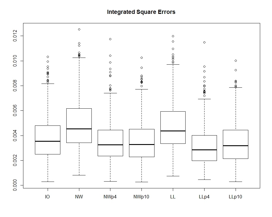
In this simulation study for carrying out the MISE analysis, we had 500 replications done using Monte Carlo method. For MISE evaluation at each combination of an estimator, a function, a standard deviation and for a fixed sample size we had to solve the optimization problem. For the numerical implementation, we used the parallel computing technique in R facilitated through ’snow’, ’doparallel’, and ’foreach’ packages.
5 Real data
In this section, we study the performance of tilted estimators in the real data environment.
5.1 COVID-19 Data
The tilted N-W estimator along with two other kernel-based estimators are being used for a curve fitting to the COVID-19 data. We shall apply the tilted N-W estimator approach to daily confirmed new cases and number of daily death for 12 countries including Iran, Australia, Italy, Belgium, Germany, Spain, Brazil, United Kingdom, Canada, Chile, South Africa and United States of America, from 23 February 2020 to 28 October 2020, downloaded from https://www.ecdc.europa.eu. The logarithmic transformation has been applied, and when the number of deaths or new confirmed cases were zero we altered these observations by a positive value eliminating the associated singularity issue. The optimal bandwidth for each Nadaraya-Watson estimator was found through minimization of relevant cross-validation function, [5], at the same time we kept the bandwidth fixed for an infinite order flat-top kernel (IO) estimator which was found using Mcmurry and Politis’ rule of thumb, [4]. Along with the tilted N-W estimator, we applied the NW, and IO estimators. The tilted NW estimator performed the best in terms of the Mean Square Errors (MSE). Table 5 and 6 provide the MSE for each estimator for the confirmed new cases and number of deaths. In terms of minimising the MSE, the tilted NW estimator ranked first, followed by IO and N-W estimators. Slightly, improved performance of the tilted NW estimator is attributed to the lower MSE components at the edges versus other kernel-based regression function estimators which are generally known for so-called "edge effect", [20]. Figures 2 and 3 shows curve fit to the daily confirmed cases and daily deaths respectively.

| Country | IO | NW | NW p4 |
|---|---|---|---|
| Iran | 324 | 326 | |
| Australia | 5.48 | 5.41 | |
| Italy | 445 | 1590 | |
| Belgium | 2357 | 3071 | |
| Germany | 641 | 1029 | |
| Spain | 41621 | 41754 | |
| Brazil | 108590 | 108246 | |
| United Kingdom | 1789 | 2083 | |
| Canada | 175 | 183 | |
| Chile | 6040 | 6685 | |
| South Africa | 1158 | 1403 | |
| United States of America | 43910 | 46512 |
| Country | IO | NW | NW p4 |
|---|---|---|---|
| Iran | 1.36 | 1.39 | |
| Australia | 0.0225 | 0.0223 | |
| Italy | 1.97 | 3.66 | |
| Belgium | 0.0699 | 0.3077 | |
| Germany | 0.71 | 0.82 | |
| Spain | 37.74 | 37.92 | |
| Brazil | 63.99 | 64.21 | |
| United Kingdom | 13.57 | 14.50 | |
| Canada | 0.40 | 0.47 | |
| Chile | 9.10 | 9.73 | |
| South Africa | 3.32 | 3.50 | |
| United States of America | 201.39 | 205.98 |

5.2 Dose-Response data
The dose-response data refers to a study of phenylephrine effects on rat corpus cavernosum strips. This data first appeared in Boroumand et al. [21] where the dose-response curves to phenylephrine (0.1 to 300 ) were obtained by applying the robust four-parameter logistic (4PL) regression. Here we have used a tilted smoother approach to dose-response curve fitting. In terms of Mean Square Errors (MSEs) the tilted local linear estimators performed better than local linear, infinite order flat-top kernel estimators including the robust 4PL model. The fitted dose-response curves using the tilted local linear, local linear, infinite order flat-top kernel estimator, and 4PL model are plotted in Figure 4. The corresponding MSEs are listed in the caption of Figure 4.

The original dose-response data contained the outliers and the standard 4PL model had a poor fit. Due to this we compared the performance of the tilted estimator with the robust 4PL model. The tilted local linear estimator outperformed the robust 4PL model in terms of MSE.
Acknowledgement
This research was undertaken with the assistance of resources and services from the National Computational Infrastructure (NCI), which is supported by the Australian Government. This research forms part of the first author’s PhD thesis approved by the ethics committee of Mashhad University of Medical Sciences with the project code 971017.
References
- [1] Andreas Buja, Trevor Hastie and Robert Tibshirani “Linear smoothers and additive models” In The Annals of Statistics JSTOR, 1989, pp. 453–510
- [2] Elizbar Nadaraya “On estimating regression” In Theory of Probability & Its Applications 9.1 SIAM, 1964, pp. 141–142
- [3] Geoffrey Watson “Smooth regression analysis” In Sankhyā: The Indian Journal of Statistics, Series A JSTOR, 1964, pp. 359–372
- [4] Timothy McMurry and Dimitris Politis “Nonparametric regression with infinite order flat-top kernels” In Journal of Nonparametric Statistics 16.3-4 Taylor & Francis, 2004, pp. 549–562
- [5] Larry Wasserman “All of nonparametric statistics” Springer Science & Business Media, 2006
- [6] Peter Hall and Qiwei Yao “Data tilting for time series” In Journal of the Royal Statistical Society: Series B (Statistical Methodology) 65.2 Wiley Online Library, 2003, pp. 425–442
- [7] Ulf Grenander “On the theory of mortality measurement: part ii” In Scandinavian Actuarial Journal 1956.2 Taylor & Francis, 1956, pp. 125–153
- [8] Art Owen “Empirical likelihood ratio confidence intervals for a single functional” In Biometrika 75.2 Oxford University Press, 1988, pp. 237–249
- [9] Song Chen “Empirical likelihood-based kernel density estimation” In Australian Journal of Statistics 39.1 Wiley Online Library, 1997, pp. 47–56
- [10] Biao Zhang “A note on kernel density estimation with auxiliary information” In Communications in Statistics-Theory and Methods 27.1 Taylor & Francis, 1998, pp. 1–11
- [11] Anton Schick and Wolfgang Wefelmeyer “Improved density estimators for invertible linear processes” In Communications in Statistics—Theory and Methods 38.16-17 Taylor & Francis, 2009, pp. 3123–3147
- [12] Ursula Müller, Anton Schick and Wolfgang Wefelmeyer “Weighted residual-based density estimators for nonlinear autoregressive models” In Statistica Sinica JSTOR, 2005, pp. 177–195
- [13] Peter Hall and Brett Presnell “Intentionally biased bootstrap methods” In Journal of the Royal Statistical Society: Series B (Statistical Methodology) 61.1 Wiley Online Library, 1999, pp. 143–158
- [14] Peter Hall and Li-Shan Huang “Nonparametric kernel regression subject to monotonicity constraints” In Annals of Statistics JSTOR, 2001, pp. 624–647
- [15] Raymond Carroll, Aurore Delaigle and Peter Hall “Testing and estimating shape-constrained nonparametric density and regression in the presence of measurement error” In Journal of the American Statistical Association 106.493 Taylor & Francis, 2011, pp. 191–202
- [16] Hassan Doosti and Peter Hall “Making a non-parametric density estimator more attractive, and more accurate, by data perturbation” In Journal of the Royal Statistical Society: Series B (Statistical Methodology) 78.2 Wiley Online Library, 2016, pp. 445–462
- [17] Hassan Doosti, Peter Hall and Jorge Mateu “Nonparametric tilted density function estimation: A cross-validation criterion” In Journal of Statistical Planning and Inference 197 Elsevier, 2018, pp. 51–68
- [18] Timothy McMurry and Dimitris Politis “Minimally biased nonparametric regression and autoregression” In REVSTAT–Statistical Journal 6.2 Citeseer, 2008, pp. 123–150
- [19] Wendy Martinez and Angel Martinez “Computational statistics handbook with MATLAB. Vol. 22” CRC press, 2007
- [20] Peter Hall and Thomas Wehrly “A geometrical method for removing edge effects from kernel-type nonparametric regression estimators” In Journal of the American Statistical Association 86.415 Taylor & Francis Group, 1991, pp. 665–672
- [21] Farzaneh Boroumand, Alireza Akbarzade, Farid Zayeri and Hediye Faghir “Application of Outlier Robust Nonlinear Mixed Effect Estimation in Examining the Effect of Phenylephrine in Rat Corpus Cavernosum” In Iranian Journal of Pharmaceutical Sciences 12.3 Iranian Association of Pharmaceutical Scientists, 2016, pp. 47–54
Appendix A Proof of Theorem 3
In this section we provide proof of Theorem 3 for tilted Nadaraya-Watson estimator as a form of tilted linear smoother from (2.3). The result for tilted local linear smoother can be proved analogously.
Proof.
Let where and is a smooth function, which is equivalent for continuous . For simplicity, we replace by then
thus for normalising so that we need to multiply the estimator (2.3) by . The factor is negligibly small. We choose such that in (2.3) is unbiased estimator for , i.e
From (A.1) we have
| (A.2) |
where
and . It can be shown that the left-hand side of (A.2) is converging to
We have
multiplying both sides by and integrating over , we deduce
by changing variable , we have
| (A.3) |
if kernel holds the assumption (c) and meet the assumption (d), then
| (A.4) |
with from (A.3), then in unbiased. Next we show that satisfies .
If the assumption (e) relaxed then there exist and , for all , , and then for unbiased
| (A.5) |
So can be written as
We recall that
- (f)
Under the assumption (e)-(1), as , so that , and under assumption (e)-(2), , where and are defined in (e)-(2).
Then under the assumption (e)-(1) and (f), we have that thus . Consequently, there exists as such that for some large since . Next, by replacing in the right-hand side of (A.5), we have a new form of (A.5) which is true for specific choice of defined at (A.3), and considering in the case of (2.3):
| (A.6) |
For this version of , does not satisfy. However, this issue can be fixed by normalisation similar to that done in the first paragraph of the proof.
Property (A.6) implies part I of Theorem 3 and part II can be concluded under uniformity of (A.6) over .
Under assumption (e)-(2) and (A.4), for , defining , we have for
so, if and , then
| (A.7) |
it means that whenever , .
In the first paragraph of the proof, we showed that . Then we found an upper bound for in (A.7) when . Now, we want to show that the probability of being out of this interval is almost zero which means for all , .
Assumption (e)-(2) implies that
| (A.8) |
Using (f), , or equivalently, , where exists. We choose so that ; or for simplicity, , then ; let , where , so
for all . Therefore by (A.8),
for all . ∎