Microscopic Patterns in the 2D Phase-Field-Crystal Model
Abstract
Using the recently developed theory of rigorously validated numerics, we address the Phase-Field-Crystal (PFC) model at the microscopic (atomistic) level. We show the existence of critical points and local minimizers associated with “classical” candidates, grain boundaries, and localized patterns. We further address the dynamical relationships between the observed patterns for fixed parameters and across parameter space, then formulate several conjectures on the dynamical connections (or orbits) between steady states.
1 Introduction
The Phase-Field-Crystal (PFC) model introduced in [1] is a gradient system capable of modeling a variety of solid-state phenomena. In its simplest form, the PFC energy can be written as
defined on phase-fields satisfying the phase constraint
The parameter represents inverse temperature such that models maximum disorder. Coupled with this energy is its conservative gradient flow which entails the sixth-order PFC equation
Note that the PFC model shares its energy with the Swift-Hohenberg equation [2], which is simply the gradient flow of . From linear stability analysis applied to single Fourier mode Ansatz, we find three main candidate global minimizers that divide parameter space, see the appendices. In the hexagonal lattice regime, 2D-simulations of the PDE starting with random noise quickly produce atoms that arrange into small patches of hexagonal lattices with random orientations. These patches grow and interact with each other, forming grains of hexagonal lattices of atoms with a particular orientation. The morphology and evolution of these grains have features resembling those in polycrystalline materials (cf. Figure 1).


In particular, it has recently been shown that statistics of many of experimentally observed (universal) grain boundary distributions are accurately captured by data amassed from simulations of this simple PFC equation [5, 4]. While here we will mostly work with this vanilla PFC formulation, we note that a family of PFC-like equations can be derived from Density-Functional-Theory [6] to obtain more complicated models capable of simulating eutectic and dendritic solidification [7] and graphene structures [8, 9].
In this article, we address the PFC model and its steady states at the “microscopic” level - the local atomic arrangement. We believe that such an investigation of microscopic pattern-formation capabilities of PFC is not only of mathematical interest but is also necessary to construct “designer” models for polycrystalline behaviour. For example, varying the parameters in the energy lead to more complicated states than simple lamellar and hexagonal. These include localized patterns in the “glassy regime” - the transition at the liquid (constant) and solid (hexagonal) transitions - and “globules” at large .
With the exception of the constant (liquid) state (cf. [10]), it is difficult to prove any theorem on the exact nature of steady states, local and global minimizers to this diffuse interface problem. What exists in the physics literature is numerical simulations, standard linear stability analysis, and Ansatz-driven energy comparisons. The recently developed theory of rigorously validated numerics (cf. [11, 12, 13, 14, 15]) now provides a powerful new tool to bridge what can be observed numerically with rigorous statements on pattern morphology. In a nutshell this approach can be summarized as follows: Given an approximate steady state, we use the Contraction Mapping Theorem to imply the existence and local uniqueness of an exact steady state within a controlled distance of the approximation. This notion of closeness is strong enough to imply further useful results, including closeness in energy and stability results. In this paper we use this new approach to address the following aspects of the PFC model:
- •
Are the “classical” candidates obtained from linear stability analysis close to actual local minimizers?
- •
Are the stable yet complicated patterns observed numerically indeed critical points in the PFC energy landscape? For example, are grain boundaries steady states or simply metastable states?
- •
What are the dynamical relationships between the observed patterns for fixed parameters and across parameter space?
Based upon our results we formulate several conjectures on the connections (or orbits) between steady states. Taken as a whole, our work presents the first step into a rigorous analysis of the rich PFC energy landscape.
The outline of this paper is as follows. We first setup the PFC equation in Fourier space and discuss the application of the framework of rigorous computations. We then verify the existence of important steady states of the PFC equation, including localized patterns and grain boundaries. With these states in hand, we address the energy landscape of PFC with a discussion on conjectures for connections (or connecting orbits) between steady states. Finally, we presents results in one-parameter numerical continuation to outline some interesting features of the bifurcation diagram of PFC.
2 PFC steady states in Fourier space
We begin by writing the equation in Fourier space to obtain a coupled system of equations for the Fourier coefficients of steady states. We will be slightly more general and consider functionals of the form
where is a linear differential operator acting on elements of a suitable function space. In particular,
where is the secondary wavelength of two-mode PFC. Taking the gradient flow of , we obtain the PFC-like equation .
For simplicity, we let be the rectangular domain with periodic boundary conditions. We let
where are the number of atoms lined up in the -axes. The main parameters of the problem are then , and the domain size is given by .
Let be the Fourier coefficients of and let be the time derivative. Inserting this expansion into the PFC equation results in an infinite system of equations of the form thanks to orthogonality. The steady states may then be found numerically by solving up to some truncation order . We will see later that it is imperative to isolate the zeros of ; the continuous translational and rotational symmetries of PFC must then be broken. The simplest way to do so in this context is to also enforce Neumann boundary conditions. It is convenient to write so that the symmetry and reality conditions become .
This choice allows us to simplify a complex Fourier series into the cosine expansion
where is a weight matrix defined by
The Fourier coefficients of are given by the elementwise product where
is the Fourier representation of the Laplacian. Inserting these expressions into the PFC equation and equating Fourier modes, we obtain
where denotes the discrete convolution and the linear terms combining and are
Note that the Fourier component picks out the average phase so it is fixed to : this is consistent with thanks to . To keep track of the phase constraint directly in , we replace its first trivial component by , resulting in:
The operator then represents the PFC dynamics in the sense that its zeros correspond to steady states of the PFC equation. A numerical advantage of the reduced expansion is that we effectively only have to compute a quarter of the full Fourier series. Obviously, this means we are not treating PFC in full generality over and will have to address this later. As an aside, the equivalent for Swift-Hohenberg is simply hence its entry is nonzero and average phase is not conserved.
3 Overview of rigorously validated numerics
We present a brief overview of the recent framework of rigorously validated numerics for dynamical systems, see sources including [11, 12, 13, 14] and [15] for a survey of techniques for PDEs.
Consider the Newton-like operator , where is a suitable inverse to the derivative . On the one hand, if is a contraction on a closed ball, the contraction mapping theorem gives the existence and uniqueness of a zero of within this ball. On the other hand, the repeated application of (allowing to vary with ) should converge to this fixed point. We can then numerically compute an approximate steady state for which up to numerical precision. If in addition we are able to show that is a contraction around , then we immediately have the existence of an exact steady state close to in an appropriate metric. This relationship is made clear by the radii polynomial theorem, so-called for reasons that will become clear shortly. To illustrate the method, we specialize the theorem to the case applicable to PFC, but see [17, 18, 19, 20] for different approaches and [21, 22] for an application to Ohta-Kawasaki functional in 2D and 3D, respectively. Given Banach spaces , we use the notation for the space of bounded linear operators from to , and for the open ball of radius around .
Theorem 1.
Consider Banach spaces , a point and let , . Suppose is Fréchet differentiable on and is injective. In addition, suppose
where are positive constants and is a positive polynomial in . Construct the radii polynomial
| (1) |
If for some , then there exists a unique for which .
The proof of this formulation is given in appendix B, where we show a correspondence between the sign of the radii polynomial and the contraction constant of : if can be found, is a contraction and the Newton iteration starting at must converge to some . This proves not only the existence of the exact steady states but also gives control on its location in with respect to a known point. In practice, one finds an interval of radii for which is negative; gives the maximum distance between while gives the minimum distance between and another zero of . The zeros of must therefore be isolated for consistency.
Each bound may be understood intuitively: being small indicates that is a good approximation of while being small indicates that is a good approximation for , and so on. These bounds may be simplified analytically but must necessarily be computed numerically. Therefore, we ensure that our numerical computations go in the same direction as the required inequalities by using interval arithmetic [23], a formalized approach to deal with numerical errors. We used the interval arithmetic package INTLAB for MATLAB, see [24, 25], to ensure that the radii polynomial approach is numerically rigorous.
This approach allows us to prepare numerical tools that can both find candidate steady states and compute the radii if they exist. If so, we immediately have a proof that this candidate provides a good handle on an actual steady state of the PFC equation.
4 Radii polynomial approach for PFC
Let us now apply these ideas to PFC by first computing and the Newton operator. Let represent the differentiation indices applied to . The derivative of is if and otherwise, so we use the Kronecker delta notation to write
For other values of , the linear terms similarly give
The derivative of the nonlinear triple convolution can be computed by differentiating with respect to all four identified by symmetry. This algebraic computation is somewhat tedious but the result can be written succinctly as
so that the full derivative of is:
and the convolutions may be viewed as infinite matrices whose “top-left” entry is the coefficient while the derivative is an infinite 4-tensor. To implement the Newton method numerically, such objects must be truncated to order such that whenever either or is greater than . This results in the matrices while the derivative becomes the 4-tensor . Note that the -convolution of has support by definition.
We now introduce the Banach space framework. Let and define as the space of sequences with finite norm
The restriction of using the symmetry condition is
over which the norm simplifies to
where is a weight matrix that forces the fast exponential decay of the Fourier coefficients. The space can easily be shown to be Banach and the 2D discrete convolution forms a Banach algebra over it, immediate results from the triangle inequality and the fact that .
Let now have the same meaning as before, with outside of thanks to the truncation. Let and denote by the numerical inverse of . We define approximate operators as
which can be thought of as block tensors containing or its inverse paired with the linear terms as the main “diagonal” of the second block. If is an invertible matrix,11 1 The numerical method will fail if is almost singular, so this is the case in practice. so is and it is thus injective. The inverse of is not however because only up to numerical inversion errors.
Note that map to a space with less regularity than because of the unbounded terms arising from real space derivatives; is a space where sequences have finite norm. However, the operator products against are bounded on thanks to the fast decay of . Thus, we say that “lifts” the regularity of the other operators back to , allowing statements such as or .
We show in appendix C how to simplify the bounds into expressions that can be evaluated numerically. This allows us to write down the radii polynomial , noting that , hence the polynomial is cubic with non-negative coefficients except for maybe the linear term. We have , and for large . As a consequence, if is strictly negative for some positive , there must exist exactly two strictly positive roots defining the interval where the proof is applicable. When this is satisfied, the radii polynomial theorem gives that
- 1.
There exists an exact solution of in .
- 2.
This solution is unique in .
Thus, when the radii polynomial is computed using interval arithmetic and has exactly two real non-negative roots, the zero computed numerically with the Newton iteration is close to an actual steady state of the PFC equation. Note the important fact that the ball is in so a priori, only the Fourier coefficients are controlled. Thanks to however, we show in appendix D that this control translates into closeness in energy and in real space norms. In particular, the distance in value between the phase fields corresponding to is at most .
Further, we show in appendix E that the stability of in is controlled by the eigenvalues of . It is important to observe that this matrix will always have a positive eigenvalue because of the trivial condition . This is not indicative of instability in the context of the gradient flow because is fixed. We shall see later that this unstable direction can be used to compute a branch of solutions in parameter continuation. For now however, we call the number of positive eigenvalues, minus , the Morse index of , indicating how many unstable directions are available to a given steady state for fixed parameters.
The procedure to numerically investigate the steady states of the PFC equation is as follows:
- •
Starting from a given initial condition, the Newton iteration is run until it converges up to numerical precision.
- •
Then, the radii polynomial of the numerical guess is computed and its roots are tested.
- •
If the proof succeeds, we can characterize an exact steady state in value, in energy and compute its stability in . The parameters can be adjusted until the proof succeeds with a trade-off between the computational effort and closeness in .
5 Rigorous results on small domains
We now have a complete framework for finding verified steady states along with their energetic and stability properties. This allows us to understand the behavior of the PFC system for a given choice of , with three important caveats:
- •
We cannot guarantee that we have found all steady states and therefore the global minimizer. Indeed, we may only hope to cover a reasonable portion of the underlying space by sampling initial conditions randomly.
- •
The size of must be balanced with to keep as small as possible, keeping in mind that is ultimately bounded above by the distance between two steady states. In particular, large domains and large increase the contribution of high frequency Fourier modes, hence the truncation order can become large even for domains containing only atoms. This limits our results to small domains so our analysis is “small scale” in nature.
- •
The Neumann boundary conditions restrict us to a “quadrant” of . While the existence of a steady state, the energy bound and instability obviously extend to , stability does not as there may be unstable directions in the other three Fourier series that are missed by the current method.
For the last point, we sometimes observe that translational shifts have a different Morse index in . This is observed for example with the stripes states, see Fig. 3 (a). In this sense, we only provide a lower bound for Morse indices in .
5.1 Verification of the candidate minimizers
The candidate global minimizers (constant, stripes, atoms and donuts states) introduced in appendix A have trivial Fourier coefficients by construction, given by
where represent amplitudes that optimize the PFC energy calculation. Note that differs between the atoms and donuts states.
To illustrate the approach, we first applied the verification program starting at the atoms state constructed for , and . The Newton iteration was used to obtain for which the radii polynomial was tested with , resulting in . The distance between and is , indeed smaller than .
The difference is mainly captured by new Fourier modes: we find that the main Fourier coefficients differ by while the largest new Fourier modes are . Moreover, the distance in the (numerical) sup norm between the two phase fields is approximately which is again smaller than the distance, consistent with the bound.
This approach was repeated for the other candidates and for a few other choices of the PFC parameters in the hexagonal regime, with truncation adjusted to . The results are presented in Table 1, showing that such simple candidates capture well the leading behavior. Note that the agreement decreases with increasing : compare the size of to .
| Ansatz | Morse index | ||||
Constant
![[Uncaptioned image]](2102.02338v1/Graphics/Small_Constant.png)
|
4 | ||||
| 16 | |||||
| 16 | |||||
Stripes
![[Uncaptioned image]](2102.02338v1/Graphics/Small_Stripes.png)
|
0 | ||||
| 7 | |||||
| 11 | |||||
Atoms
![[Uncaptioned image]](2102.02338v1/Graphics/Small_Atoms.png)
|
0 | ||||
| 0 | |||||
| 0 | |||||
Donuts
![[Uncaptioned image]](2102.02338v1/Graphics/Small_Donuts.png)
|
3 | ||||
| 12 | |||||
| 16 |
5.2 Steady states in the hexagonal lattice regime
The Newton iteration can detect new steady states regardless of stability as it is based on criticality instead of minimality. This allows us to find steady states that are observed only momentarily or even locally during a PFC simulation. Table 2 presents a few of the distinct steady states found for , , and . Starting at random initial coefficient matrices, the Newton iteration converges in 15 to 50 steps. The four main ansatz were also explicitly tested, as only the atoms state could be reached from random initial conditions.
| Visualization | Morse index | Count | ||
![[Uncaptioned image]](2102.02338v1/Graphics/SS_LargeDomain_1.png)
|
||||
![[Uncaptioned image]](2102.02338v1/Graphics/SS_LargeDomain_3.png)
|
||||
![[Uncaptioned image]](2102.02338v1/Graphics/SS_LargeDomain_8.png)
|
||||
![[Uncaptioned image]](2102.02338v1/Graphics/SS_LargeDomain_22.png)
|
||||
![[Uncaptioned image]](2102.02338v1/Graphics/SS_LargeDomain_42.png)
|
Note that the energy of the exact steady states can be compared from Table 2: for instance, the energy of the exact atoms state is bounded away from the others so it is guaranteed to be the best candidate global minimizer out of the observed steady states at the current parameter values.
The second and third states presented in the table clearly display two grains of the same orientation but with boundary atoms meeting “head-to-head.” This is essentially an intermediate in the grains slipping on one another that is stabilized by the restrictions of the boundary conditions. Such states then represent a grain boundary that is stable, at least in . When PFC simulations [26] are initialized at these states, the flow appears to be stable for thousands of steps then suddenly goes to the hexagonal lattice, meaning there are unstable directions in the rest of . Nevertheless, the fact remains that grain boundaries can be steady states.
5.3 Steady states in the localized patterns regime
Table 3 presents some steady states found for , , and . In this regime, localized or coexistence patterns are observed in PFC simulations, some of which we can confirm to be steady states: note in particular the existence of a “single atom” state. We see here that the global minimizer cannot be of the four main ansatz. We observe two atoms states with different amplitudes and stability, highlighting the fact that the “linear” candidate is no longer appropriate as increases and nonlinear effects begin to dominate the energy.
Similar results have been obtained previously for a version of Swift-Hohenberg with broken symmetry, see [27, 28].
| Visualization | Morse index | ||
![[Uncaptioned image]](2102.02338v1/Graphics/SS_Localized_0.png)
|
|||
![[Uncaptioned image]](2102.02338v1/Graphics/SS_Localized_2.png)
|
|||
![[Uncaptioned image]](2102.02338v1/Graphics/SS_Localized_7.png)
|
|||
![[Uncaptioned image]](2102.02338v1/Graphics/SS_Localized_5.png)
|
|||
![[Uncaptioned image]](2102.02338v1/Graphics/SS_Localized_6.png)
|
|||
|
|
5.4 Steady states for the large regime
Table 4 shows a selection of steady states found in the large regime, , , and . In this regime, the microscopic organization is lost as constant patches of phase form, with value close to , meaning that the double well term of the PFC functional dominates the oscillation term.
| Visualization | Morse index | ||
![[Uncaptioned image]](2102.02338v1/Graphics/SS_LargeBeta_1.png)
|
|||
![[Uncaptioned image]](2102.02338v1/Graphics/SS_LargeBeta_2.png)
|
|||
![[Uncaptioned image]](2102.02338v1/Graphics/SS_LargeBeta_3.png)
|
|||
![[Uncaptioned image]](2102.02338v1/Graphics/SS_LargeBeta_5.png)
|
5.5 Phase diagram with verified steady states
The framework allows us to construct a “rigorous” phase diagram for PFC. Here the adjective “rigorous” does not mean that we have identified the ground state; but rather that the respective candidate state has been rigorously verified in its parameter regime. To this end, one must construct a “patchwork” of split in regions in which we have a proof that a given state is a global minimizer. For now, we restrict ourselves to proving that one of the steady states near the known candidate minimizers has lower energy than all other known steady states at given points. Further, our attempt is somewhat limited by the small domains we can access. Nevertheless, this construction is useful and does indicate rigorously where the candidates cannot be global minimizers.
Our approach is as follows: we discretize the parameter space to some desired accuracy and for each point, we test the four ansatz and several other candidates obtained from random initial coefficients. When one of the four ansatz has verified lower energy than the others, up to translational symmetries, we label that point accordingly and otherwise leave the point blank. Fig. 2 (a) shows the resulting diagram for small parameter values with , , . At each point, trials of the Newton iteration were tried and verified rigorously. Note that the points below could have been skipped since the constant state is known to be the global minimizer in that regime [10]. This diagram matches the one obtained in the appendices with linear stability analysis.
Fig. 2 (b) shows the phase diagram near where localized patterns have been observed. The domain is the same size but to accommodate the larger . At each point, trials were tried and verified, leading to points that have lower energy than the atoms or constant states. This indeed shows the existence of a region where localized patterns are more energetically favourable. This region gives an estimate of the full coexistence region that ultimately cannot be made explicit without more refined techniques.


5.6 Rigorous results for two-mode PFC
As a final example, Table 5 shows three verified steady states for two-mode PFC with , , , and . Note that here, to fit the symmetry of the square lattice. The second state shows two grains slipping on each other; in contrast, especially to the result for hexagonal lattices, the third state is a grain boundary with non-zero misorientation. Here, the rectangular domains with Neumann boundary conditions can support the geometry of the square lattice at and rotations, so we can observe their coexistence. Since this result can be extended to larger domains by simple tiling operations, we conclude that straight grain boundaries can be steady states even in infinite domains where boundary conditions cannot “help” stabilizing such defects.
Moreover, this grain boundary was observed to be (numerically) stable in two-mode PFC simulations in the sense that small random perturbations of the phase field always converged back to the grain boundary state. This is not a rigorous proof of stability in , but it gives a good indication that grain boundaries are likely to be stable features in the PFC model.
| Visualization | Morse index | ||
![[Uncaptioned image]](2102.02338v1/Graphics/SS_Square_1.png)
|
|||
![[Uncaptioned image]](2102.02338v1/Graphics/SS_Square_2.png)
|
|||
![[Uncaptioned image]](2102.02338v1/Graphics/SS_Square_3.png)
|
6 Connections between steady states
Suppose represent two steady states, we say that there is a connection (or a connecting orbit) from to if there exists a solution with the property that
More precisely, the connecting orbit leaves the unstable manifold of and ends up in the stable manifold of . Since the PFC equation is a gradient flow, there cannot exist non-trivial homoclinic connections so there is a natural hierarchy of steady states expressed through heteroclinic connections. This concept is extremely useful to “visualize” the energy landscape.
States with Morse index are stable (for fixed parameters) and are thus at the bottom of the hierarchy. Those states with Morse index have one unstable direction, so there are two distinct perturbations that lead away from the state. For states with Morse index , two unstable directions span infinitely many such perturbations, and so on. To detect connections, we propose to initialize a PFC flow near an unstable steady state offset by such perturbations. If the flow becomes close enough to another known steady states, we stop and propose a conjectured connection between the two steady states. This procedure often allows us to find unknown steady states: when the flow stagnates, the Newton iteration can be run and often converges in very few steps to a steady state that can be verified. Alternatively, we could check for inclusion in the target ball, but this is a very restrictive criterion that limits our numerical investigation, especially when obtaining connections to unstable states. We use the PFC scheme detailed in [26].
While we cannot for the moment prove such claims because “parameterizing” the infinite dimensional stable manifold of the unstable steady states is highly non-trivial, we are aware of some preliminary work in this direction [29]. That said, computer-assisted proofs of connecting orbits from saddle points to asymptotically stable steady states in parabolic PDEs are starting to appear [30, 31, 32].
We first consider the standard parameters and use the very small domain . This choice is made to ensure that the constant state has Morse index in to simplify the visualization. We find seven steady states: both possible translations of the atoms, stripes and donuts state, and the trivial constant state. Following the program described above, we can construct the “connection diagram” shown in Fig. 3 (a) with the arrows indicating that a connection was found from a state to the other. Note in particular that the stable stripes state to the right numerically decays into the appropriately shifted hexagonal lattices, but this is a slow process as the sine modes must grow out of numerical noise. This clearly shows that our method cannot be used to guarantee stability in because it cannot depend on translational shifts.


We also propose a visualization method for such diagrams shown in Fig. 3 (b). Take for example the constant state with its two unstable directions given by the coefficients and . We place the constant state at the origin and plot radial lines along linear combination of the unstable directions. The line length corresponds to the number of PFC steps needed to approach the target steady states. In addition, we can color the points along the line as a function of energy to indicate energetic relationships. A variant would be to show the energy as the -component of a surface; essentially giving an indirect visualization of the energy landscape through 2D unstable manifolds. In particular, this diagram clarifies the relationships between the steady states. For instance, the stripes states are formed by adding the mode to the constant state while the donuts are combinations of the atoms and stripes states.
We now consider the localized patterns regime to illustrate these ideas with states of high Morse index. We do not attempt to build a higher dimensional visualization, but simply attempt to recover the “pathways” between the highly unstable hexagonal lattice with Morse index towards stable steady states. This is visualized in the connection diagram of Fig. 4 (a) which includes a few states of Table 3. In (b), we plot the energy along the PFC flow starting from the index 2 state; this plot can be thought of as one of the rays in a diagram like Fig. 3 (b). Note that along the flow, the energy decreases in “steps” corresponding to changes in topology, i.e. the formation (or removal) of atoms. In this process, we could not verify that these intermediates are steady states since the Newton iteration always converged to the endpoint; we then suppose they are short-lived “metastable” states.
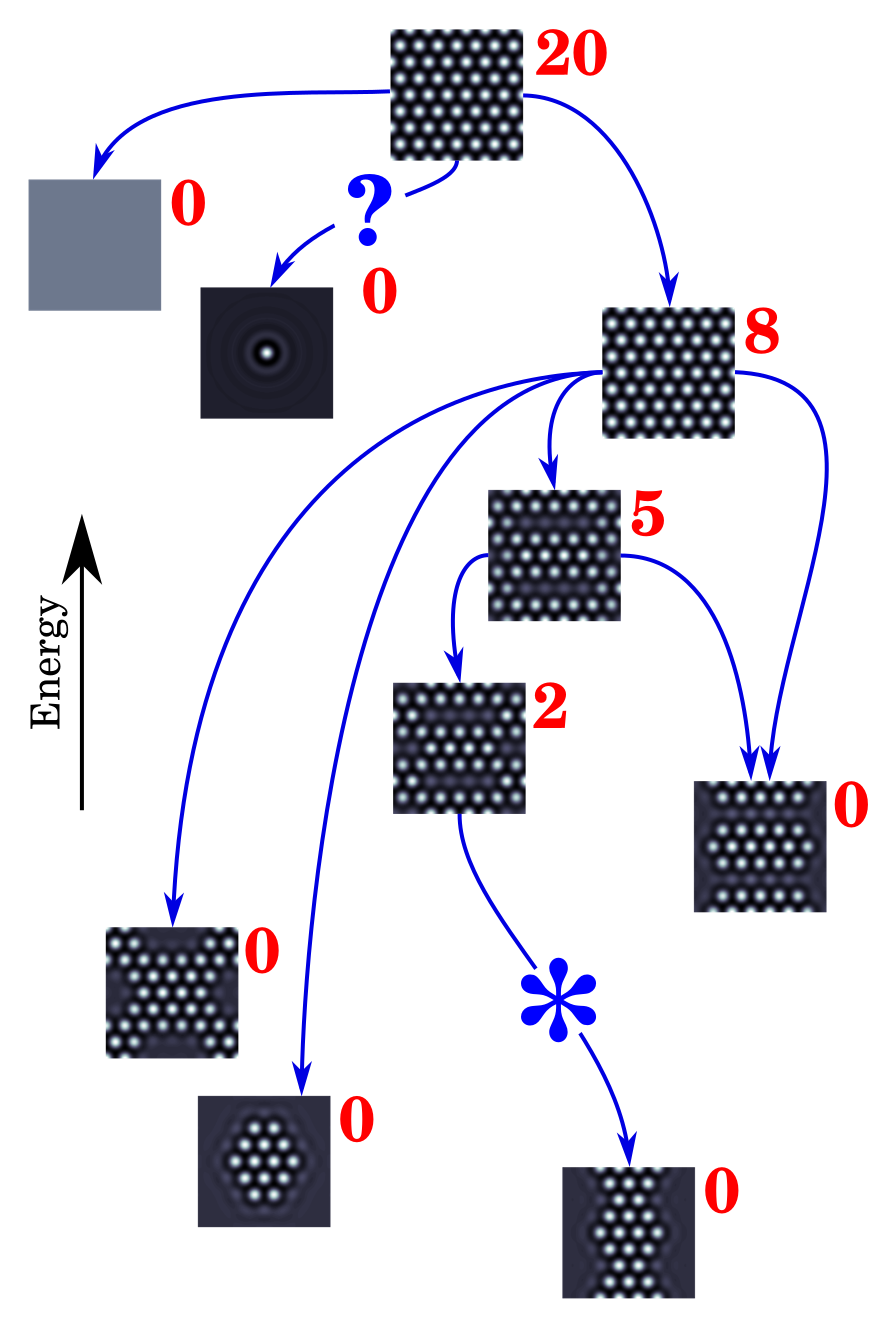

It is difficult to obtain perturbations that can flow to desired steady states, especially when they are unstable; see how only a few directions reach the Morse index states in Fig. 3 (b). Indeed, unless “trivial” combinations of the unstable direction happen to go to an unstable state, we are unlikely to find such connections numerically. Similarly, our attempts to find a perturbation that connects the starting lattice to the single atom state were unfruitful.
7 Parameter continuation for steady states
A verified steady state for some parameter is usually part of a family of steady states representing a “phase” of matter. In fact, the candidate minimizers defined in appendix A as functions of approximate such families, or branches in the bifurcation diagram. In this context, we can construct such branches by starting at a known steady state, vary and find the closest steady state at this new parameter value.
Several verified techniques exist for following branches, see [33] and [21] for an application to Ohta-Kawasaki. We use non-verified pseudo-arclength continuation [34] in . Note that the unstable direction that is to followed is precisely given by the one corresponding to the “fixed” condition and this is one of the reasons that we chose to enforce this directly in the formulation of . As a possible extension, 2D manifolds can be constructed in 2-parameter continuation when both parameters are allowed to vary, see [35].
Fig. 5 shows the norm (a) and offset energy (b) of the main ansatz at are plotted as functions of . The domain is kept small with to keep the bifurcation diagram as simple as possible. The atoms and donuts branches are actually the same since we can continue the branches through the folds at . This branch intersects the checkers state at and the constant and stripes states at . The energy plot (b) clearly shows that the donuts state is the “proper” hexagonal lattice for . We note that varying simply causes the branches to dilate. For example, we expect the 2D hexagonal steady states manifold to be a “conic” figure-eight.


Other “new” branches will appear for larger domains or higher . In particular, Fig. 6 shows the atoms/donuts branch and the single atom branch in the localized patterns regime near with . Again, (a) shows the norm and (b) shows the energy of the phase field as functions of . The hexagonal lattice traces out its usual figure-eight pattern while the single atom (and other localized states in general) traces out a complicated looping path. Such branches illustrate the “snaking” phenomenon previously observed in modified Swift-Hohenberg equations that support such localized patterns, see [27] for example. We observe that the path loops on itself in one direction as the single atom evolves into a localized pattern with , then atoms before looping back with a rotation. In the other direction, the branch moves towards the transition between the hexagonal and constant states where it again loops back. This computation is difficult because the truncation must remain large and the pseudo-arclength step size must remain small; if the step size is larger than , the branch breaks away towards the hexagonal lattice solution.


8 Conclusion
We surveyed the basic properties of the PFC equation as a dynamical system in the framework of rigorous numerics. Thanks to an application of the radii polynomial approach, we were able to verify the existence of steady states close to numerically computed approximations. This provided us with important verified information as to the behavior of the energy landscape, especially in terms of energetic relationships between steady states. We were also able to provide partial stability results with the caveat that they only applied to the cosine Fourier series. The Morse indices given were lower bounds in - thus those steady states with Morse index higher than 0 must be unstable in .
Such ideas were applied in various regimes of the PFC equation to verify that certain important patterns are steady states (as opposed to metastable intermediates) including single atoms, other localized patterns and grain boundaries. In particular, we showed that two-mode PFC supports a non-zero misorientation grain boundary steady state that we expect to be stable. We also showed the construction of the phase diagram with our fully nonlinear approach.
Finally, we used such results to further investigate the energy landscape through connections or orbits and through parameter continuation. Connections reveal the energetic and dynamical relationships between steady states, highlighting the behavior of unstable patterns as they reach states with lower energy. Continuation is especially useful to understand how the important states evolve across parameter space, highlighting the surprising behavior of the hexagonal lattice patterns and the snaking behavior of localized patterns.
Our work suggests several interesting directions for future work. On one hand, our connection results could be made rigorous with a technique to prove orbits from unstable to stable manifolds. This is a complicated problem because the stable manifold is infinite dimensional and special techniques must be applied to properly parameterize its “dominant” submanifold. On the other, our continuation results could also be made rigorous or extended to 2-parameter continuation to reveal more interesting behavior. Alternatively, parameter continuation could be applied to the domain size, for example to investigate problems in elasticity.
References
- [1] K. R. Elder, M. Katakowski, M. Haataja, and M. Grant, “Modeling elasticity in crystal growth,” Physical Review Letters, vol. 88, p. 245701, 2002.
- [2] J. Swift and P. C. Hohenberg, “Hydrodynamic fluctuations at the convective instability,” Physical Review A, vol. 15, pp. 319–328, 1977.
- [3] G. Martine La Boissonière and R. Choksi, “Atom based grain extraction and measurement of geometric properties,” Modelling and Simulation in Materials Science and Engineering, vol. 26, no. 3, p. 035001, 2018.
- [4] G. Martine La Boissonière, R. Choksi, K. Barmak, and S. Esedoḡlu, “Statistics of grain growth: experiment versus the Phase-Field-Crystal and Mullins models,” Materialia, p. 100280, 2019.
- [5] R. Backofen, K. Barmak, K. E. Elder, and A. Voigt, “Capturing the complex physics behind universal grain size distributions in thin metallic films,” Acta Materialia, vol. 64, pp. 72–77, 2014.
- [6] H. Emmerich, H. Löwen, R. Wittkowski, T. Gruhn, G. I. Tóth, G. Tegze, and L. Gránásy, “Phase-field-crystal models for condensed matter dynamics on atomic length and diffusive time scales: an overview,” Advances in Physics, vol. 61, no. 6, pp. 665–743, 2012.
- [7] M. Greenwood, N. Ofori-Opoku, J. Rottler, and N. Provatas, “Modeling structural transformations in binary alloys with phase field crystals,” Physical Review B, vol. 84, no. 6, p. 064104, 2011.
- [8] M. Seymour and N. Provatas, “Structural phase field crystal approach for modeling graphene and other two-dimensional structures,” Physical Review B, vol. 93, p. 035447, 2016.
- [9] P. Hirvonen, M. M. Ervasti, Z. Fan, M. Jalalvand, M. Seymour, S. M. V. Allaei, N. Provatas, A. Harju, K. R. Elder, and T. Ala-Nissila, “Multiscale modeling of polycrystalline graphene: a comparison of structure and defect energies of realistic samples from phase field crystal models,” Physical Review B, vol. 94, no. 3, p. 035414, 2016.
- [10] D. Shirokoff, R. Choksi, and J.-C. Nave, “Sufficient conditions for global minimality of metastable states in a class of non-convex functionals: a simple approach via quadratic lower bounds,” Journal of Nonlinear Science, vol. 25, no. 3, pp. 539–582, 2015.
- [11] H. Koch, A. Schenkel, and P. Wittwer, “Computer-assisted proofs in analysis and programming in logic: a case study,” SIAM Review, vol. 38, no. 4, pp. 565–604, 1996.
- [12] M. T. Nakao, “Numerical verification methods for solutions of ordinary and partial differential equations,” Numerical Functional Analysis and Optimization, vol. 22, no. 3-4, pp. 321–356, 2001.
- [13] W. Tucker, Validated numerics: a short introduction to rigorous computations. Princeton University Press, 2011.
- [14] J. B. van den Berg and J. P. Lessard, “Rigorous numerics in dynamics,” Notices of the American Mathematical Society, vol. 62, no. 9, pp. 1057–1061, 2015.
- [15] J. Gómez-Serrano, “Computer-assisted proofs in PDE: a survey,” SeMA Journal, pp. 1–26, 2018.
- [16] K. A. Wu, A. Adland, and A. Karma, “Phase-field-crystal model for FCC ordering,” Physical Review E, vol. 81, no. 6, p. 061601, 2010.
- [17] S. Day, J.-P. Lessard, and K. Mischaikow, “Validated continuation for equilibria of PDEs,” SIAM Journal on Numerical Analysis, vol. 45, no. 4, pp. 1398–1424, 2007.
- [18] A. Hungria, J. P. Lessard, and J. D. Mireles James, “Rigorous numerics for analytic solutions of differential equations: the radii polynomial approach,” Mathematics of Computation, vol. 85, no. 299, pp. 1427–1459, 2016.
- [19] I. Balázs, J. B. van den Berg, J. Courtois, J. Dudás, J. P. Lessard, A. Vörös-Kiss, J. F. Williams, and X. Y. Yin, “Computer-assisted proofs for radially symmetric solutions of PDEs,” Journal of Computational Dynamics, vol. 5, no. 1-2, pp. 61–80, 2018.
- [20] J. B. van den Berg, “Introduction to rigorous numerics in dynamics: general functional analytic setup and an example that forces chaos,” Rigorous Numerics in Dynamics, Proceedings of Symposia in Applied Mathematics, vol. 74, pp. 1–25, 2017.
- [21] J. B. van den Berg and J. F. Williams, “Validation of the bifurcation diagram in the 2D Ohta-Kawasaki problem,” Nonlinearity, vol. 30, no. 4, p. 1584, 2017.
- [22] J. B. van den Berg and J. F. Williams, “Rigorously computing symmetric stationary states of the Ohta-Kawasaki problem in three dimensions,” SIAM J. Math. Anal., vol. 51, no. 1, pp. 131–158, 2017=9.
- [23] R. E. Moore, Interval analysis, vol. 4. Prentice-Hall, 1966.
- [24] S. M. Rump, “INTLAB - interval laboratory,” in Developments in Reliable Computing, pp. 77–104, Springer, 1999.
- [25] G. I. Hargreaves, “Interval analysis in MATLAB,” Numerical Algorithms, no. 2009.1, 2002.
- [26] M. Elsey and B. Wirth, “A simple and efficient scheme for phase field crystal simulation,” ESAIM: Mathematical Modelling and Numerical Analysis, vol. 47, no. 5, pp. 1413–1432, 2013.
- [27] D. J. B. Lloyd, B. Sandstede, D. Avitabile, and A. R. Champneys, “Localized hexagon patterns of the planar Swift-Hohenberg equation,” SIAM Journal on Applied Dynamical Systems, vol. 7, no. 3, pp. 1049–1100, 2008.
- [28] J. B. van den Berg, A. Deschênes, J. P. Lessard, and J. D. Mireles James, “Stationary coexistence of hexagons and rolls via rigorous computations,” SIAM Journal on Applied Dynamical Systems, vol. 14, no. 2, pp. 942–979, 2015.
- [29] J. van den Berg, J. Jaquette, and J. Mireles James, “Validated numerical approximation of stable manifolds for parabolic partial differential equations.” Preprint, 2020.
- [30] J. Cyranka and T. Wanner, “Computer-assisted proof of heteroclinic connections in the one-dimensional Ohta-Kawasaki Model,” SIAM J. Appl. Dyn. Syst., vol. 17, no. 1, pp. 694–731, 2018.
- [31] C. Reinhardt and J. D. Mireles James, “Fourier-Taylor parameterization of unstable manifolds for parabolic partial differential equations: formalism, implementation and rigorous validation,” Indag. Math. (N.S.), vol. 30, no. 1, pp. 39–80, 2019.
- [32] J. Jaquette, J.-P. Lessard, and A. Takayasu, “Global dynamics in nonconservative nonlinear Schrödinger equations.” Preprint, 2020.
- [33] J. B. van den Berg, J. P. Lessard, and K. Mischaikow, “Global smooth solution curves using rigorous branch following,” Mathematics of Computation, vol. 79, no. 271, pp. 1565–1584, 2010.
- [34] H. B. Keller, Lectures on numerical methods in bifurcation problems, vol. 79 of Tata Institute of Fundamental Research Lectures on Mathematics and Physics. Published for the Tata Institute of Fundamental Research, Bombay, 1987. With notes by A. K. Nandakumaran and Mythily Ramaswamy.
- [35] M. Gameiro, J. P. Lessard, and A. Pugliese, “Computation of smooth manifolds via rigorous multi-parameter continuation in infinite dimensions,” Foundations of Computational Mathematics, vol. 16, no. 2, pp. 531–575, 2016.
Appendices
A PFC ansatz in 2D
PFC simulations can be classified according to a small number of regimes or ansatz that represent the (expected) global minimizer. The choice of such candidates is motivated by numerical experiments but can be obtained analytically from techniques such as linear stability analysis. Consider a periodic “single Fourier mode” phase field of the form
on the rectangular domain . Inserting this ansatz into the PFC energy yields an expression that can be optimized in the three amplitudes. This procedure yields three main classes of states that are well-known in the PFC literature.
- •
The constant state .
- •
The stripes state and .
- •
The hexagonal lattice states .
In addition, we also find a “checkers state” where and are given as more complicated expressions. The two hexagonal lattices differ in energy: the positive choice is called the “donuts” state while the negative one is the “atoms” state. We can compare the energies directly to show that the checkers state is never optimal while the atoms state is more optimal than the donuts state for .
When the coefficients of two candidates are equal, they represent the same regime; for example, at , the constant, stripes and donuts states are all . Similarly, the donuts and atoms states merge at . We can also compute when states have the same energy. Such behavior occurs on transition curves of the form .
We can construct the phase diagram in Fig. 7 by labeling with the expected global minimizer. We show in the main text that this “linear” description of PFC is a good approximation, at least for small .


B Proof of the radii polynomial theorem
Proof.
Consider the Newton operator , then and any fixed point of is a zero of because is injective. The derivative of is bounded and also Fréchet differentiable since we have for any
as is the (bounded linear) Fréchet derivative of . Now suppose for some , then the radii polynomial in the main text gives
since is positive.
Let , we can use the previous inequality to bound
Pairing this with the mean value inequality for ,
hence maps to its interior thanks to the strict inequality. Similarly for ,
so is a contraction with constant and the Banach fixed-point theorem gives the result. ∎
C Computation of the radii polynomial bounds
In the following calculations, we will use usual results such as
and the following proposition to compute the norm of operators on :
Proposition 1.
Let be an operator such that whenever , then
Proof.
Let , then can be decomposed as the action of the first finite block onto for and infinitely many diagonal terms for . The norm of can then be written as the sum of two disjoint positive sums using the triangle inequality:
The second term is bounded by the trivial bound , extracting the norm of over . Similarly, the first term is bounded by
The norm of in is the supremum of the previous norm over all with unit norm, therefore the triangle inequality gives the result. ∎
The sharper result can be obtained by noting that the sums act on different subspaces of . The estimate also allows us to compute the norm of finite tensors by letting the vanish. Let us now apply these results to compute the four necessary bounds.
C.1 bound
This bound is the easiest since by construction, are approximate inverses up to numerical inversion errors. We then have
which can be evaluated using proposition 1.
C.2 bound
We must compute so that most terms will be given by the finite product . There still remain some non-zero convolution coefficients in the full : since has coefficients in each dimension, will have non-zero coefficients in each dimension. These are multiplied by the appropriate , resulting in
C.3 bound
To compute the bound, let with and consider first the effect of on ,
Fix and let where , we then have that
Note that the initial factor can instead be represented by the diagonal operator defined by . Then, using the fact that the convolution on is a Banach algebra,
where the norm of is computed using proposition 1 with the bound on the diagonal terms.22 2 This can be done since is monotone decreasing as long as either or can dominate the term. For PFC, so a sufficiently large ensures that or dominates . This condition can be checked numerically. This computation works for any , so we have
C.4 bound
For the final bound, we now consider the action of on the same vector :
Let be the tail of , i.e. the vector with the same entries as outside of and on . We then have:
Consider now the action of on the difference above. The first block of the difference will be multiplied by the inverse of while the tail will be multiplied by the appropriate , thus
using and the triangle inequality for the first term.
Let be such that whenever and otherwise. Using the Banach algebra property and the bound to bound the infinite sum, we have
which can be computed numerically once the (finitely many) have been obtained. To compute them, we now shift for a moment to and extend all vectors appropriately. Now let , then
where are the regions over which and are non-zero respectively. Since whenever either or is larger than and we only need , we obtain the overestimate that . Further, must vanish for so
for (and otherwise), which completes the computation of .
D Energy computation and real space norms
The notion of closeness between and extends to their energies. For simplicity, we only handle the basic PFC energy
We will write without relabeling when is the phase field corresponding to the Fourier coefficients . Taking the average of a Fourier series returns its constant mode such that
In the context of the radii polynomial approach, let such that
We can simplify by integrating by parts and using the periodic boundary conditions; for example,
We now use the fact that . In addition, we can overestimate and use the Banach algebra property to obtain the following bound:
The term strictly in has been left as a convolution because it is necessary to control the growth of with the bound directly. To do so, we have
which is another way to obtain the previous integration by parts result. Now, the norm of is bounded by ; each member of the sum satisfies the inequality . Overestimating , we can write
where . To evaluate this sum, we can compute the polynomial geometric series
which all converge for . Note that the sums can be evaluated by differentiating with respect to . The terms in can then be expanded and written in such a fashion and assuming that is finite, the sums can be split and separated. We have
and similarly,
| (2) |
Putting everything together, we arrive at the bound
which can now be computed numerically. This bound depends strongly on because of its influence on and the growth of . In principle, one could find an optimal that ensures the bound is as small as possible for a given and a fixed .
When the numerical errors associated to the computations are added to the energy bound, both computed with interval arithmetic, we obtain an interval that is guaranteed to contain the energy of itself. In particular, this allows us to prove which of two steady states is more optimal33 3 The energy intervals must be disjoint for such statements to hold. Otherwise, the proof parameters must be improved to tighten the intervals. strictly from numerical computations.
The previous computations illustrate some techniques that allow us to estimate the norm of (the phase field corresponding to ) in terms of . For example,
| (3) |
provides a pointwise estimate on the value of the exact steady state. Further, a simple calculation shows that Parseval’s identity holds on ; i.e. . We can then bound the norm of derivatives, for instance
using Eq. (2). Similar results can be built for the lower norms, thus providing an estimate of the form
for some constant that could be computed if necessary. Note the implicit dependence on the state itself and through . Combined with the bound, this shows that as long as , the exact steady state will be in and can differ from the numerical candidate by at most at any point in . The constant may be large, but it does not affect the pointwise agreement; this is sufficient control for our numerical investigation.
E Stability in
To complete the analysis of a given steady state , we can characterize its stability in . This is powerful because even linear results are mostly limited to trivial states but a major limitation is that this does not transfer to because is restricted to the cosine series.
Suppose we have a steady state for a verified radius , then stability is controlled by the spectrum of . This spectrum is real because we are in the context of a gradient flow; this can be seen directly from the definition of which are symmetric on interchanging indices. Assuming there are no zero eigenvalues, the positive and negative ones define the unstable and stable manifolds respectively. A steady state with only strictly negative eigenvalues is said to be stable.
While only the approximation is known in practice, it has the same signature as itself; i.e. they have exactly as many strictly positive or strictly negative eigenvalues. We compute the spectrum of in two parts. The eigenvalues of the finite block can be computed numerically and verified using interval arithmetic routines.44 4 This verification is numerically costly for large truncation order; when , we only verify the eigenvalues that are larger than some arbitrary lower bound, say Most eigenvalues can be unequivocally assigned a sign, but some may be identically or closer to than the available precision. Stability cannot be ascertained in such cases, but assuming was verified using the radii polynomial approach, must be sufficiently well-conditioned so its eigenvalues cannot be so small.
In the tail, the eigenvalues are simply equal to the diagonal terms with . Thankfully, is strictly negative for and is strictly positive as long as is sufficiently large. We then have
which can be split into a finite number of positive eigenvalues and infinitely many negative eigenvalues, assuming there are no small eigenvalues. The equivalence with follows from a homotopy argument. Let for , then
as in the proof of the radii polynomial approach. Since is a bounded operator with norm less than , is itself invertible. and thus cannot have a zero eigenvalue so that its signature must stay constant for all . This shows that have the same signature and this is in fact true over the ball of radius around .