Numerical Differentiation using local Chebyshev-Approximation
Abstract
1 Motivation
In applied mathematics, especially in optimization, functions are often only provided as so called ”Black-Boxes” provided by software packages, or very complex algorithms, which make automatic differentation very complicated or even impossible. Hence one seeks the numerical approximation of the derivative.
Unfortunately numerical differentation is a difficult task in itself, and it is well known that it is numerical instable. There are many works on this topic, including the usage of (global) Chebyshev approximations. Chebyshev approximations have the great property that they converge very fast, if the function is smooth. Nevertheless those approches have several drawbacks, since in practice functions are not smooth, and a global approximation needs many function evalutions.
Nevertheless there is hope. Since functions in real world applications are most times smooth except for finite points, corners or edges. This motivates to use a local Chebyshev approach, where the function is only approximated locally, and hence the Chebyshev approximations still yields a fast approximation of the desired function. We will study such an approch in this work, and will provide a numerical example.
Disclaimer: This work was done as private research during my study years and is not related to my current affiliation at all. No funding was recieved for this work.
2 Chebyshev Polynomials and One Dimensional Functions
First we recall some well known definitions. the following definitions and properties are taken from [1].
Definition 2.1 (Chebyshev-Polynomials).
For the -th Chebyshev polynomial is given by . From this definition we see that the Chebyshev polynomial takes it’s extrema at
The points are the so called Gauss-Lobatto Grid-points.
The best way to approximate functions via Chebyshev-polynomials lies in the following
Proposition 2.2 (Chebyshev-Series & Co).
Set , then
forms the (weighted) scalar product of the Hilbert-Space
Then for a function the Chebyshev-Coefficients
exists, and the Chebyshev-Series
converges in the sense to .
Proof.
These well known facts follow from applying classical Fourier-theory to
. ∎
Since Chebyshev-Polynomials are “cosines in disguise” other important properties from Fourier-theory carry over to Chebyshev-series, like spectral convergence for smooth functions etc.
Another way to approximate a function is to use the Chebyshev-Interpolation Polynomial , which is uniquely defined by for .
Although the Chebyshev-Series yields the best approximation there is a little known fact between the two approximation types, namely the
Proposition 2.3.
Let a function with
and
Further let for ,
be the trunctation error, and Then
and for the interpolation error
Hence the penalty for using interpolation instead of truncation is at most a factor of two! Additionally the coefficients of the interpolation polynomial are related to the exact coefficents by the identity
| (1) |
That means the approximated coefficients differ from the exact coefficients by the aliasing-error, and hence the error vanishes with
Proof.
See [1, Thm. 6& Thm. 21]. ∎
Since with Chebyshev interpolation we are close to the realm of the DFT, additional methods from signal processing, like denoising could be considered to handle numerical distortions.
To work with a function a generalized Chebyshev interpolation for can be achieved by using a linear transformation , and interpolate the function .
Since computing the derivative of a polynomial can be done exactly we could use the derivative of for some , as the numerical derivative of . This means
Then how about the errors? First recall the identity . Hence for the truncation error we have
Considering that has it’s extrema at with , we immediately see that
For the interpolation polynomial we get by using the aliasing identity (1) and rearranging terms like in the proof of [1, Thm. 21] the error estimation
Hence we have the
Proposition 2.4.
For smooth we have the error estimation
Hence the penalty for using interpolation instead of truncation when differentiating is at most a factor of two!
3 Practical Considerations in the 1D Case and Generalizations
In this section consider a function , which is continuous and piecewise smooth, but not differentiable in a set of finite points (with finite and allowed to be empty).
If we interpolate now the function on the interval , we know from Fourier-Theory, that the error will converge only slowly to zero. We also note that it is easy to see that (from variable transformations) that error estimation depends on the length of the interval . with the factor . Hence if one restricts the function only on a small interval, one achieves more precise interpolation results, with lesser degrees of the interpolation polynomial. If we restrict the function to some interval , with
- 1.
and
- 2.
for ,
then the sequence of the Chebyshev interpolation polynomials converges very fast (with spectral convergence) and uniformly to the original function in the interval .
From Proposition 2.4 we know that this then also applies to , since the error decays with . Nevertheless we also see that for practical use it is important to ensure the smoothness on the observed interval , because of the term . This leads to the following definition
Definition 3.1.
Let be continuous and piecewise smooth, then we call the Chebyshev interpolation polynomial of the local smooth Chebyshev polynomial iff
This motivates the following algortithm to compute derivatives of a function (if the points are known):
As one can see we also included more general derivatives based on directional derivatives like subgradients. It also would be possible to define a weak derivative witch is motivated by Chebyshev convergence theory defined by .
A question which still remains, is what to do when the set is unknown. This is still an open problem, but since one can observe the speed of the decay of the coefficients (or ) it is possible to locate non differentiable points. There are several works on this topic from spectral theory.
Now to the dimensional case: Consider a functional , which is continuous and piecewise smooth on the domain . We can compute the directional derivatives in a direction in a point by deriving the one dimensional function . Hence the methods from the one dimensional case, can be carried over to the dimensional setting.
4 Examples
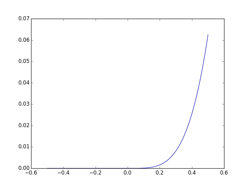
as first we define the function given by (see also Figure 1):
First we compare computing the first derivative with local Chebyshev approximation with finite differences given by
by computing the values at and . See Table 1 for results. As we can observe the errors of and are equal. This comes without surprise, since the derivative of the rd Chebyshev polynomial is exactly the central difference quotient.
Next we will modify in the following way: For some , and a randomly standard normal distributed variable we define by
and then try to differentiate it at . the results can be seen at Table 2.
The errors are maximal values after taking some samples (There is some space for improvement here, e.g. better statistics, but we get the picture…) We Observe the following behavior: While and behave like expected, we see that making smaller, does not make the approximation quality of and better, but even worse. This can be explained by the fact, that for smooth , we know that the function behaves like it’s Taylor polynomial of lower order, while the higher order terms are neglectable. This also means that computing a higher order Chebyshev polynomial does not make sense, and we even get into more trouble. hence when choosing a suitable for the Chebyshev approximation should be not too small, and yet not too big.
Finally we try the Local Chebyshev Method on the 2D Rosenbrock function
with parameters and , and try to find the minimum with help of gradient methods. The argmin is Additionally we add some disturbances and in the interval . While is some randomly normal distributed variable, is a jump function which changes it’s sign (which is fatal for finite differences). As optimization method we used Steepest Descent with Armijo-rule and as terminating criterion. We used for the finite difference method, and order polynomials with for the Local Chebyshev Method. and The number of iterations and the computed results (rounded up to 3 digits) can be seen in Table 3. The results suggest, that computing the gradient with the Local Chebyshev Method makes the algorithm more robust. Also it was observed that the stepsize should be not too small.
| Function | Method | Iteration Numbers | Result |
|---|---|---|---|
| Exact Gradient | |||
| Finite Differences | |||
| Local-Chebyshev | |||
| Finite Differences | (interrupted) | ||
| Local-Chebyshev | |||
| Finite Differences | (interrupted) | ||
| Local-Chebyshev |
References
- [1] Boyd, John P. Chebyshev and Fourier spectral methods. Courier Corporation, 2001.