The ${\rm SL}(2,\mathbb{C})$ -character variety of a Montesinos knot

Haimiao Chen

Abstract

For each Montesinos knot $K$ , we propose an efficient method to explicitly determine the irreducible ${\rm SL}(2,\mathbb{C})$ -character variety, and show that it can be decomposed as $\mathcal{X}_{0}(K)\sqcup\mathcal{X}_{1}(K)\sqcup\mathcal{X}_{2}(K)\sqcup\mathcal{X}^{\prime}(K)$ , where $\mathcal{X}_{0}(K)$ consists of trace-free characters, $\mathcal{X}_{1}(K)$ consists of characters of “unions” of representations of rational knots (or rational link, which appears at most once), $\mathcal{X}_{2}(K)$ is an algebraic curve, and $\mathcal{X}^{\prime}(K)$ consists of finitely many points when $K$ satisfies a generic condition.

Keywords: ${\rm SL}(2,\mathbb{C})$ -character variety; irreducible representation; Montesinos knot; rational tangle
MSC2020: 57K10, 57K31

1 Introduction

Let $G={\rm SL}(2,\mathbb{C})$ and let $\Gamma$ be a finitely presented group. A $G$ -representation of $\Gamma$ is a homomorphism $\rho:\Gamma\to G$ . The $G$ -representation variety of $\Gamma$ is $\mathcal{R}_{G}(\Gamma):=\hom(\Gamma,G)$ . Call a representation $\rho$ reducible if elements in ${\rm Im}(\rho)$ have a common eigenvector, which is equivalent to ${\rm Im}(\rho)\subset\mathbf{a}U\mathbf{a}^{-1}$ for some $\mathbf{a}\in G$ , where $U$ denotes the subgroup of $G$ consisting of upper-triangular matrices; in particular, call $\rho$ abelian if ${\rm Im}(\rho)$ is abelian. Call $\rho$ irreducible if $\rho$ is not reducible. Let $\mathcal{R}^{\rm irr}_{G}(\Gamma)$ denote the space of irreducible representations.

The character of $\rho$ is by definition the function $\chi_{\rho}:\Gamma\to\mathbb{C}$ , $g\mapsto{\rm tr}(\rho(g)).$ As a fact ([6] Proposition 1.5.2), two irreducible representations $\rho,\rho^{\prime}$ are conjugate (meaning that there exists $\mathbf{a}\in G$ such that $\rho^{\prime}(x)=\mathbf{a}\rho(x)\mathbf{a}^{-1}$ for all $x\in\Gamma$ ) if and only if $\chi_{\rho}=\chi_{\rho^{\prime}}$ . Focusing on irreducible representations, the (irreducible) $G$ -character variety of $\Gamma$ is $\mathcal{X}^{\rm irr}_{G}(\Gamma)=\{\chi_{\rho}\colon\rho\in\mathcal{R}^{\rm irr}_{G}(\Gamma)\}.$

When $\Gamma=\pi(L):=\pi_{1}(S^{3}-L)$ for a link $L$ , we call $\mathcal{X}^{\rm irr}_{G}(\Gamma)$ the $G$ -character variety of $L$ , and so on. Throughout the paper, we usually work directly on representations, which are more convenient. A representation whose conjugacy ambiguity is fixed will always be identified with its character.

There are many reasons for caring about representations. Here are two of them. First, in general, having a representation $\rho:\pi(L)\to{\rm GL}(d,\mathbb{F})$ , one can define the twisted Alexander polynomial of $L$ associated to $\rho$ , which is useful in many situations (referred to [7] and the references therein). Second, nowadays a popular topic is the left orderability of $\pi_{1}(M)$ for 3-manifolds $M$ ; here a group $G$ is called left-orderable if it admits a total ordering $<$ such that $g<h$ implies $fg<fh$ for all $f,g,h\in G$ . For a 3-manifold $M$ resulting from a Dehn surgery on a knot $K$ , a systematic approach to understanding the left orderability of $\pi_{1}(M)$ was proposed by Culler-Dunfield [5], by using continuous paths of ${\rm SL}(2,\mathbb{R})$ -representations of $K$ .

Computing character varieties of links is a notoriously difficult problem. The importance for computation lies in that knowledge on character variety is still too limited, and concrete results may give directions for further research. Till now, character varieties have been determined for only a few links. Existing results include: torus knots [11], double twist knots [10], double twist links [13], $(-2,2m+1,2n)$ -pretzel links and twisted Whitehead links [15], and classical pretzel knots [3, 4]. Recently, the result of [3] was applied by Khan and Tran [9] to show left orderability for some Dehn surgeries on odd pretzel knots.

As a related work, in [12] Paoluzzi and Porti studied the ${\rm SL}(2,\mathbb{C})$ -character varieties of Montesinos knots of Kinoshita-Terasaka type using the “bending trick”, to reveal some interesting phenomena; for instance, the character variety contains a $d$ -dimensional component for each $d$ in a certain range.

In this article, we show

Theorem 1.1.

For each Montesinos knot $K$ , the irreducible character variety has a decomposition $\mathcal{X}^{\rm irr}_{{\rm SL}(2,\mathbb{C})}(K)=\mathcal{X}_{0}(K)\sqcup\mathcal{X}_{1}(K)\sqcup\mathcal{X}_{2}(K)\sqcup\mathcal{X}^{\prime}(K),$ where

•

$\mathcal{X}_{0}(K)$ consists of trace-free characters;
•

$\mathcal{X}_{1}(K)$ consists of characters of “unions” of representations of rational knots or maybe one rational link;
•

$\mathcal{X}_{2}(K)$ is a high-genus algebraic curve, whose defining equation can be written down;
•

$\mathcal{X}^{\prime}(K)$ is a finite set when $K$ satisfies a generic condition.

The “generic condition” for $K$ is precisely stated in Proposition 4.6.

Actually we give an efficient method for determining the character variety. The techniques used are elementary, but the results are amazing. Each of the four parts $\mathcal{X}_{0}(K),\mathcal{X}_{1}(K),\mathcal{X}_{2}(K),\mathcal{X}^{\prime}(K)$ has distinguishable feature. When the number $m$ of strands of $K$ is larger than 3, many new phenomena appear, in contrast to $m=3$ . $\mathcal{X}_{1}(K)$ is concerned with representations from $F_{m}$ (the free group on $m$ generators) to ${\rm SL}(2,\mathbb{C})$ . The last part $\mathcal{X}^{\prime}(K)$ is rather subtle, and can be regarded as certain kind of singularity, which we manage to handle.

This is the first time to systematically deal with a class of knots whose fundamental groups can have arbitrarily many generators. The structural description of $\mathcal{X}^{\rm irr}_{{\rm SL}(2,\mathbb{C})}(K)$ provides necessary conditions for deciding whether a given knot is Montesinos, which in general is a difficult problem [8]. Explicit descriptions will provide plenty of examples on character varieties; in particular, examples of character varieties having high-dimensional components.

The paper is organized as follows. Section 2 is a collection of basic notions. In Section 3, representations of rational tangles are investigated in detail; some fine things are clarified and several useful formulas are derived. In Section 4, a method for finding all irreducible representations for each Montesinos knot is developed, and then Theorem 1.1 is established. We assume that the values of characters taken at meridians are nonzero, since the case when the values vanish had been worked out in [2].

2 Preparation

2.1 Tangles and links

We adopt the notations and conventions used in [2].

By a tangle we simultaneously mean an un-oriented tangle diagram and the 1-dimensional manifold embedded in $\mathbb{R}^{3}$ it stands for.

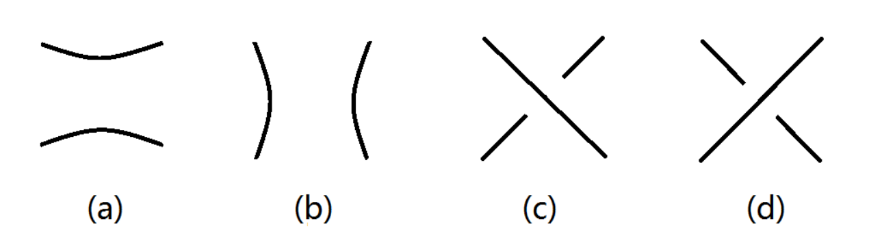
Refer to caption — Figure 1: Four elements in $\mathcal{T}_{2}^{2}$ : (a) $[0]$ , (b) $[\infty]$ , (c) $[1]$ , (d) $[-1]$ .

Let $\mathcal{T}_{2}^{2}$ denote the set of 4-ended tangles. Four of the simplest elements of $\mathcal{T}_{2}^{2}$ are $[0]$ , $[\infty]$ , $[1]$ , $[-1]$ , as shown in Figure 1. Defined on $\mathcal{T}_{2}^{2}$ are horizontal composition $+$ and vertical composition $\ast$ , as illustrated in Figure 2.

For $k\neq 0$ , the horizontal composite of $|k|$ copies of $[1]$ (resp. $[-1]$ ) is denoted by $[k]$ if $k>0$ (resp. $k<0$ ), and the vertical composite of $|k|$ copies of $[1]$ (resp. $[-1]$ ) is denoted by $[1/k]$ if $k>0$ (resp. $k<0$ ). Given $k_{1},\ldots,k_{s}\in\mathbb{Z}$ , the rational tangle $[[k_{1}],\ldots,[k_{s}]]$ is defined as

\begin{cases}[k_{1}]\ast[1/k_{2}]+\cdots+[k_{s}],&2\nmid s,\\ [1/k_{1}]+[k_{2}]\ast\cdots+[k_{s}],&2\mid s.\end{cases}

The fraction of the tangle $[[k_{1}],\ldots,[k_{s}]]$ is given by the continued fraction $[[k_{1},\ldots,k_{s}]]\in\mathbb{Q}$ , which is defined inductively as

[[k_{1}]]=k_{1};\qquad[[k_{1},\ldots,k_{j}]]=k_{j}+1/[[k_{1},\ldots,k_{j-1}]],\quad 2\leq j\leq s.

Denote the tangle $[[k_{1}],\ldots,[k_{s}]]$ as $[p/q]$ when its fraction equals $p/q$ , where $p$ is coprime to $q$ , and call it odd (resp. even) if $p$ is odd (resp. even).

Each $T\in\mathcal{T}_{2}^{2}$ gives rise to two links: the numerator $N(T)$ and the denominator $D(T)$ , as shown in Figure 3. For $p/q\in\mathbb{Q}$ , the link $N([p/q])$ is called a rational link or 2-bridge link, which has one component (resp. two components) if $p$ is odd (resp. even). A link of the form $D([p_{1}/q_{1}]\ast\cdots\ast[p_{m}/q_{m}])$ is called a Montesinos link and denoted by $M(p_{1}/q_{1},\ldots,p_{m}/q_{m})$ ; in particular, $M(p_{1},\ldots,p_{m})$ is a pretzel link.

Convention 2.1.

An Montesinos knot $M(p_{1}/q_{1},\ldots,p_{m}/q_{m})$ is called odd if $2\nmid p_{i}$ for all $i$ , and called even if $2\mid p_{i}$ for exactly one $i$ . In the second case, by cyclically permuting the indices, we always assume $2\mid p_{m}$ . Even Montesinos knots are the same as those of Kinoshita-Terasaka type.

Note that the northwest and northeast end of $[p_{i}/q_{i}]$ belong to the same component if and only if $M(p_{1}/q_{1},\ldots,p_{m}/q_{m})$ is even and $i=m$ .

2.2 On $2\times 2$ matrices

We use bold letters to denote elements of ${\rm SL}(2,\mathbb{C})$ .

Introduce some special elements:

	$\displaystyle\mathbf{e}=\left(\begin{array}[]{cc}1&0\\ 0&1\end{array}\right),\qquad\mathbf{p}=\left(\begin{array}[]{cc}1&1\\ 0&1\end{array}\right),\qquad\mathbf{w}=\left(\begin{array}[]{cc}0&1\\ -1&0\end{array}\right),$
	$\displaystyle\mathbf{d}(\kappa)=\left(\begin{array}[]{cc}\kappa&0\\ 0&\kappa^{-1}\end{array}\right),\quad\mathbf{u}^{+}_{\kappa}(\xi)=\left(\begin{array}[]{cc}\kappa&\xi\\ 0&\kappa^{-1}\end{array}\right),\quad\mathbf{u}_{\kappa}^{-}(\xi)=\left(\begin{array}[]{cc}\kappa&0\\ \xi&\kappa^{-1}\end{array}\right).$

The Weyl element $\mathbf{w}$ has the property that $\mathbf{w}\mathbf{x}\mathbf{w}^{-1}=(\mathbf{x}^{\prime})^{-1}$ for each $\mathbf{x}$ , where $\mathbf{x}^{\prime}$ denotes the transpose of $\mathbf{x}$ .

Let $M$ denote the set of $2\times 2$ matrices. Let $U$ denote the subgroup of ${\rm SL}(2,\mathbb{C})$ consisting of upper-triangular elements.

For $\lambda$ with $\lambda+\lambda^{-1}\neq t^{2}-2,\pm 2$ and $\mu\neq 0$ , put

\displaystyle\mathbf{h}_{t}^{\lambda}(\mu)=\frac{1}{\lambda+1}\left(\begin{array}[]{cc}\lambda t&\mu\\ (t^{2}-\lambda-\lambda^{-1}-2)\lambda\mu^{-1}&t\end{array}\right).

For $t\neq 0$ , put

\displaystyle\mathbf{k}_{t}(\alpha)=\left(\begin{array}[]{cc}t/2+\alpha&(t^{2}/4-1-\alpha^{2})/(2t)\\ 2t&t/2-\alpha\end{array}\right).

Direct computation leads to

	$\displaystyle{\rm tr}\big(\mathbf{h}_{t}^{\lambda}(\mu)^{-1}\mathbf{h}_{t}^{\lambda}(\nu)\big)$	$\displaystyle=\frac{2t^{2}+(\lambda+\lambda^{-1}+2-t^{2})(\mu\nu^{-1}+\mu^{-1}\nu)}{\lambda+\lambda^{-1}+2},$		(1)
	$\displaystyle{\rm tr}\big(\mathbf{k}_{t}(\alpha)^{-1}\mathbf{k}_{t}(\beta)\big)$	$\displaystyle=2+(\alpha-\beta)^{2}.$		(2)

The reason for introducing these matrices is clear from the following lemma.

Lemma 2.2.

Suppose $\mathbf{a}_{1},\mathbf{a}_{2}\in{\rm SL}(2,\mathbb{C})$ with ${\rm tr}(\mathbf{a}_{1})={\rm tr}(\mathbf{a}_{2})=t$ .

(a)

If $\mathbf{a}_{1}\mathbf{a}_{2}=\mathbf{d}(\lambda)$ with $\lambda+\lambda^{-1}\neq t^{2}-2,\pm 2$ , then $\mathbf{a}_{1}=\mathbf{h}_{t}^{\lambda}(\mu)$ and $\mathbf{a}_{2}=\mathbf{h}_{t}^{\lambda}(-\lambda^{-1}\mu)$ for some $\mu\neq 0$ .
(b)

If $\mathbf{a}_{1}\mathbf{a}_{2}=\mathbf{p}$ , then $\mathbf{a}_{1},\mathbf{a}_{2}\in U$ .
(c)

If $\mathbf{a}_{1}\mathbf{a}_{2}=-\mathbf{p}$ and $t\neq 0$ , then $\mathbf{a}_{1}=\mathbf{k}_{t}(\alpha)$ and $\mathbf{a}_{2}=\mathbf{k}_{t}(\alpha-t)$ for some $\alpha$ .
(d)

$\mathbf{a}_{1}$ and $\mathbf{a}_{2}$ have a common eigenvector if and only if ${\rm tr}(\mathbf{a}_{1}\mathbf{a}_{2})\in\{2,t^{2}-2\}$ .

Proof.

Suppose $\mathbf{a}_{i}=\left(\begin{array}[]{cc}a_{i}&b_{i}\\ c_{i}&d_{i}\end{array}\right)$ , with $a_{i}d_{i}-b_{i}c_{i}=1$ and $a_{i}+d_{i}=t.$

(a) It follows from $\mathbf{a}_{2}=\mathbf{a}_{1}^{-1}\mathbf{d}(\lambda)$ that $a_{2}=\lambda d_{1}$ and $d_{2}=\lambda^{-1}a_{1}$ , so

\displaystyle a_{i}=\frac{\lambda t}{\lambda+1},\qquad d_{i}=\frac{t}{\lambda+1},\qquad b_{i}c_{i}=\frac{t^{2}-\lambda-\lambda^{-1}-2}{\lambda+\lambda^{-1}+2}\neq 0.

Hence $\mathbf{a}_{1}=\mathbf{h}_{t}^{\lambda}(\mu)$ and $\mathbf{a}_{2}=\mathbf{h}_{t}^{\lambda}(-\lambda^{-1}\mu)$ , with $\mu=(\lambda+1)b_{1}$ .

(b) It follows from $\mathbf{a}_{2}=\mathbf{a}_{1}^{-1}\mathbf{p}$ that $a_{2}=d_{1}$ and $d_{2}=a_{1}-c_{1}$ , so $c_{1}=0$ . Then $c_{2}=0$ , too.

(c) It follows from $\mathbf{a}_{2}=-\mathbf{a}_{1}^{-1}\mathbf{p}$ that $a_{2}=-d_{1}$ and $d_{2}=c_{1}-a_{1}$ , so $c_{1}=2t$ . Hence $\mathbf{a}_{1}=\mathbf{k}_{t}(\alpha)$ and $\mathbf{a}_{2}=\mathbf{k}_{t}(\lambda-t)$ , with $\alpha=a_{1}-t/2$ .

(d) ( $\Rightarrow$ ) is obvious.

For ( $\Leftarrow$ ), suppose ${\rm tr}(\mathbf{a}_{1}\mathbf{a}_{2})\in\{2,t^{2}-2\}$ . Replacing $\mathbf{a}_{1}$ by $\mathbf{a}_{1}^{-1}$ if necessary, we may assume ${\rm tr}(\mathbf{a}_{1}\mathbf{a}_{2})=2$ . If $\mathbf{a}_{1}\mathbf{a}_{2}\neq\mathbf{e}$ , then up to conjugacy we may assume $\mathbf{a}_{1}\mathbf{a}_{2}=\mathbf{p}$ . By (b), $\mathbf{a}_{1}$ shares an eigenvector with $\mathbf{a}_{2}$ . ∎

Remark 2.3.

In the generic case, whenever ${\rm tr}(\mathbf{a}_{1}\mathbf{a}_{2})=\lambda+\lambda^{-1}$ , up to conjugacy we may assume $\mathbf{a}_{1}\mathbf{a}_{2}=\mathbf{d}(\lambda)$ , so that $\mathbf{a}_{1}=\mathbf{h}_{t}^{\lambda}(\mu)$ and $\mathbf{a}_{2}=\mathbf{h}_{t}^{\lambda}(-\lambda^{-1}\mu)$ for some $\mu\neq 0$ . This will simplify computations in many situations.

For $r=\eta+\eta^{-1}$ and $n\in\mathbb{Z}$ , put

	$\displaystyle\omega_{n}(r)$	$\displaystyle=\begin{cases}(\eta^{n}-\eta^{-n})/(\eta-\eta^{-1}),&\eta\notin\{\pm 1\},\\ n\eta^{n-1},&\eta\in\{\pm 1\},\end{cases}$
	$\displaystyle\theta_{n}(r)$	$\displaystyle=\eta^{n}+\eta^{-n}.$

For any $\mathbf{z}\in{\rm SL}(2,\mathbb{C})$ , by repeated applications of Hamilton-Cayley Theorem,

\displaystyle\mathbf{z}^{n}=\omega_{n}({\rm tr}(\mathbf{z}))\mathbf{z}-\omega_{n-1}({\rm tr}(\mathbf{z}))\mathbf{e}.

(3)

3 Representations of rational tangles

Given a tangle $T$ , let $\mathfrak{D}(T)$ denote the set of directed arcs of $T$ ; each arc gives rise to two directed arcs. If the directed arcs $a,b$ belong to the same component of $T$ (regarded as an embedded 1-manifold), then denote $[a]=[b]$ (resp. $[a]=-[b]$ ) if their directions are the same (resp. the opposite). By a representation of $T$ , we mean a map $\rho:\mathfrak{D}(T)\to{\rm SL}(2,\mathbb{C})$ such that $\rho(a^{-1})=\rho(a)^{-1}$ for each $a\in\mathfrak{D}(T)$ , and $\rho(c)=\rho(a)\rho(b)\rho(a)^{-1}$ for each crossing as illustrated in Figure 4. To present such a representation, it is sufficient to give each arc a direction and label an element of ${\rm SL}(2,\mathbb{C})$ beside it. We say that $\rho$ is trace- $t$ if ${\rm tr}(\rho(a))=t$ for each $a\in\mathfrak{D}(T)$ .

In virtue of Wirtinger presentation, a representation $\rho$ of $T$ can be identified with a true representation $\rho:\pi_{1}(B-T)\to{\rm SL}(2,\mathbb{C})$ , where $B$ is a 3-ball containing $T$ such that $\partial B\cap T$ exactly consists of the end points of $T$ .

Given a representation $\rho$ of $T\in\mathcal{T}_{2}^{2}$ , let

\displaystyle\mathbf{x}^{{\rm nw}}=\rho(T^{{\rm nw}}),\qquad

\displaystyle\mathbf{x}^{{\rm ne}}=\rho(T^{{\rm ne}}),\qquad\mathbf{x}^{{\rm sw}}=\rho(T^{{\rm sw}}),\qquad\mathbf{x}^{{\rm se}}=\rho(T^{{\rm se}}),

where $T^{{\rm nw}}$ , $T^{{\rm ne}}$ , $T^{{\rm sw}}$ , $T^{{\rm se}}$ are respectively the northwest, northeast, southwest, southeast ends of $T$ , all directed outward. Clearly, $\mathbf{x}^{{\rm nw}}\mathbf{x}^{{\rm ne}}\mathbf{x}^{{\rm se}}\mathbf{x}^{{\rm sw}}=\mathbf{e}$ , so that $\mathbf{x}^{{\rm nw}}\mathbf{x}^{{\rm ne}}=(\mathbf{x}^{{\rm sw}})^{-1}(\mathbf{x}^{{\rm se}})^{-1}$ . Let

z={\rm tr}(\mathbf{x}^{{\rm nw}}\mathbf{x}^{{\rm ne}})-2,\qquad\dot{z}={\rm tr}(\mathbf{x}^{{\rm nw}}\mathbf{x}^{{\rm sw}})-2,\qquad\grave{z}={\rm tr}(\mathbf{x}^{{\rm nw}}\mathbf{x}^{{\rm se}})-2.

3.1 Some useful formulas

From now on till the end of this section, let $T=[[k_{1}],\ldots,[k_{s}]]$ be a rational tangle, some of whose directed arcs are illustrated in Figure 5. We use a normal letter $a$ to denote a directed arc, and use boldface one $\mathbf{a}$ to denote the value $\rho$ takes at $a$ . Let $x=T^{\rm nw}=(x^{(0)})^{(-1)^{s}}$ and $y=(y^{(0)})^{\pm 1}$ , where the sign is chosen to make $[y]=[T^{\rm ne}]$ or $[y]=[T^{\rm sw}]$ if $\pm[x]=[T^{\rm ne}]$ . Suppose $\rho$ is a representation of $T$ . Call $(\mathbf{x},\mathbf{y})$ the generating pair for $\rho$ . Let $t={\rm tr}(\mathbf{x})={\rm tr}(\mathbf{y})$ and $r={\rm tr}(\mathbf{x}\mathbf{y})$ .

Lemma 3.1.

$\mathbf{y}$ can be written as a word in $\mathbf{x}^{\rm ne}$ , $\mathbf{x}^{\rm sw}$ , $\mathbf{x}^{\rm se}$ . Consequently, $\rho$ is determined by $\mathbf{x}^{\rm nw}$ , $\mathbf{x}^{\rm ne}$ , $\mathbf{x}^{\rm sw}$ , $\mathbf{x}^{\rm se}$ .

Proof.

By induction on $i$ , starting with $i=0$ , it is easy to show that $\mathbf{x}^{(s-i)},\mathbf{y}^{(s-i)}$ can be written as words in $\mathbf{e},\mathbf{x}^{\rm ne},\mathbf{x}^{\rm sw},\mathbf{x}^{\rm se}$ . ∎

Using (3) and the identity

\mathbf{y}\mathbf{x}=(r-t^{2})\mathbf{e}+t(\mathbf{x}+\mathbf{y})-\mathbf{x}\mathbf{y},

in principle we can recursively compute $\mathbf{x}^{(j)},\mathbf{y}^{(j)}$ , $j=1,\ldots,s$ , writing each one as a linear combination of $\mathbf{e},\mathbf{x},\mathbf{y},\mathbf{x}\mathbf{y}$ , with coefficients in $\mathbb{Z}[t,r]$ , and then obtain $z,\dot{z},\grave{z}\in\mathbb{Z}[t,r]$ . However, such computations are usually tedious, and they are unnecessary for our purpose. Here we take a better approach to derive the formulas for $z,\dot{z},\grave{z}$ .

For $\gamma,\nu\neq 0$ and $n\in\mathbb{Z}$ , introduce

\displaystyle\psi_{\gamma}^{\nu}(n)=\frac{2t^{2}+(2-\nu-\nu^{-1}-t^{2})(\nu^{n}\gamma+\nu^{-n}\gamma^{-1})}{2-\nu-\nu^{-1}}.

Let

-\nu_{j}-\nu_{j}^{-1}=e_{j}={\rm tr}\big(\mathbf{x}^{(-1)^{j}}\mathbf{y}^{(j)}\big),\qquad 0\leq j\leq s-1.

In the generic case, up to conjugacy we may assume $\mathbf{x}^{(0)}=\mathbf{h}_{t}^{-\nu_{0}}(1)$ , $\mathbf{y}^{(0)}=\mathbf{h}_{t}^{-\nu_{0}}(\nu_{0}^{-1})$ . Then $\mathbf{y}^{(1)}=\mathbf{h}_{t}^{-\nu_{0}}(\nu_{0}^{k_{1}})$ , $\mathbf{x}^{(1)}=\mathbf{h}_{t}^{-\nu_{0}}(\nu_{0}^{k_{1}-1})^{-1}$ , and by (1),

e_{1}=\psi_{1}^{\nu_{0}}(k_{1}),\qquad{\rm tr}\big(\mathbf{x}^{(0)}\mathbf{x}^{(1)}\big)=\psi_{1}^{\nu_{0}}(k_{1}-1).

Up to another conjugacy, we may assume $(\mathbf{x}^{(0)})^{-1}=\mathbf{h}_{t}^{-\nu_{1}}(1)$ , $\mathbf{y}^{(1)}=\mathbf{h}_{t}^{-\nu_{1}}(\nu_{1}^{-1})$ , and moreover, $\mathbf{y}^{(0)}=\mathbf{h}_{t}^{-\nu_{1}}(\gamma_{1})$ , $\mathbf{x}^{(1)}=\mathbf{h}_{t}^{-\nu_{1}}(\nu_{1}^{-1}\gamma_{1})$ for some $\gamma_{1}$ . Then

\displaystyle e_{0}=\psi_{\gamma_{1}}^{\nu_{1}}(0),\qquad{\rm tr}\big(\mathbf{x}^{(0)}\mathbf{x}^{(1)}\big)=\psi_{\gamma_{1}}^{\nu_{1}}(-1).

From $\psi_{\gamma_{1}}^{\nu_{1}}(0)=e_{0}$ and $\psi_{\gamma_{1}}^{\nu_{1}}(-1)={\rm tr}\big(\mathbf{x}^{(0)}\mathbf{x}^{(1)}\big)=\psi_{1}^{\nu_{0}}(k_{1}-1)$ we obtain

\Big(1-\frac{t^{2}}{2+e_{1}}\Big)\gamma_{1}^{\pm 1}=\frac{\nu_{1}^{\pm 1}e_{0}-\psi_{1}^{\nu_{0}}(k_{1}-1)}{\nu_{1}^{\pm 1}-\nu_{1}^{\mp 1}}+\frac{2t^{2}}{(\nu_{1}^{\pm 1}-\nu_{1}^{\mp 1})(1-\nu_{1}^{\mp 1})}.

Consequently, for each $n\in\mathbb{Z}$ ,

	$\displaystyle\psi_{\gamma_{1}}^{\nu_{1}}(n)$	$\displaystyle=\Big(1-\frac{t^{2}}{2+e_{1}}\Big)\gamma_{1}\nu_{1}^{n}+\Big(1-\frac{t^{2}}{2+e_{1}}\Big)\gamma_{1}^{-1}\nu_{1}^{-n}+\frac{2t^{2}}{2+e_{1}}$
		$\displaystyle=e_{0}\omega_{n+1}(-e_{1})-\psi_{1}^{\nu_{0}}(k_{1}-1)\omega_{n}(-e_{1})+\frac{2t^{2}}{2+e_{1}}(1-\omega_{n+1}(-e_{1})+\omega_{n}(-e_{1})).$

Moreover, $\mathbf{y}^{(2)}=\mathbf{h}_{t}^{-\nu_{1}}(\nu_{1}^{k_{2}}\gamma_{1})$ , $\mathbf{x}^{(2)}=\mathbf{h}_{t}^{-\nu_{1}}(\nu_{1}^{k_{2}-1}\gamma_{1})^{-1}$ , and

e_{2}=\psi_{\gamma_{1}}^{\nu_{1}}(k_{2}),\qquad{\rm tr}\big((\mathbf{x}^{(0)})^{-1}\mathbf{x}^{(2)}\big)=\psi_{\gamma_{1}}^{\nu_{1}}(k_{2}-1).

Going on, up to yet another conjugacy, we may assume

\mathbf{x}^{(0)}=\mathbf{h}_{t}^{-\nu_{2}}(1),\ \ \ \mathbf{y}^{(2)}=\mathbf{h}_{t}^{-\nu_{2}}(\nu_{2}^{-1}),\ \ \ \mathbf{y}^{(1)}=\mathbf{h}_{t}^{-\nu_{2}}(\gamma_{2}),\ \ \ \mathbf{x}^{(2)}=\mathbf{h}_{t}^{-\nu_{2}}(\nu_{2}^{-1}\gamma_{2}),

for some $\gamma_{2}$ . Then

\displaystyle e_{1}=\psi_{\gamma_{2}}^{\nu_{2}}(0),\qquad{\rm tr}\big((\mathbf{x}^{(0)})^{-1}\mathbf{x}^{(2)}\big)=\psi_{\gamma_{2}}^{\nu_{2}}(-1),

which, similarly as above, imply that for each $n\in\mathbb{Z}$ ,

\displaystyle\psi_{\gamma_{2}}^{\nu_{2}}(n)=e_{1}\omega_{n+1}(-e_{2})-\psi_{\gamma_{1}}^{\nu_{1}}(k_{2}-1)\omega_{n}(-e_{2})+\frac{2t^{2}}{2+e_{2}}(1-\omega_{n+1}(-e_{2})+\omega_{n}(-e_{2})).

In general, there exist $\gamma_{0}=1$ and $\gamma_{1},\ldots,\gamma_{s-1}\in\mathbb{C}^{\ast}$ such that, with $\psi_{\gamma_{j}}^{\nu_{j}}(n)$ abbreviated to $\psi_{j}(n)$ ,

$\displaystyle\psi_{0}(n)$	$\displaystyle=\theta_{n}(-e_{0})+\frac{2-\theta_{n}(-e_{0})}{2+e_{0}}t^{2},$	(4)
$\displaystyle e_{j}$	$\displaystyle=\psi_{j-1}(k_{j}),\qquad 1\leq j\leq s-1,$	(5)
$\displaystyle\psi_{j}(n)$	$\displaystyle=e_{j-1}\omega_{n+1}(-e_{j})-\psi_{j-1}(k_{j}-1)\omega_{n}(-e_{j})+\frac{2t^{2}(1-\omega_{n+1}(-e_{j})+\omega_{n}(-e_{j}))}{2+e_{j}}.$	(6)

So the $\psi_{j}(n)$ ’s can be recursively computed as a polynomial in $t$ and $r$ , without explicitly referring to $\gamma_{j}$ . In particular, we can obtain the expressions for

\dot{z}=e_{s-1}-2,\qquad\grave{z}=\psi_{s-1}(k_{s}-1)-2,\qquad z=\psi_{s-1}(k_{s})-2.

Note that these equations are polynomial equations. Since they are available under some Zariski open conditions, actually they always hold.

Remark 3.2.

When $t=0$ , (4)–(6) can be much simplified and can lead to closed formulas for $z,\dot{z},\grave{z}$ in terms of $\nu_{0}$ .

Write $t=\kappa+\kappa^{-1}$ . If $T$ is odd, then $N(T)$ is a knot. We assert that

z=(r-2)\phi_{N(T)}(\kappa,2-r)^{2},

where $\phi_{N(T)}(\kappa,u)$ is the Riley polynomial of $N(T)$ , as introduced in [14].

It can be shown that $x^{\rm ne}=vyv^{-1}$ for some word

v=(y^{-1})^{\epsilon_{1}}x^{\epsilon_{2}}\cdots(y^{-1})^{\epsilon_{2h-1}}x^{\epsilon_{2h}},\qquad\text{with}\quad\epsilon_{i}=\epsilon_{2h+1-i}\in\{\pm 1\}.

For a nonabelian representation of $N(T)$ , up to conjugacy one may assume $\mathbf{x}=\mathbf{u}^{-}_{\kappa}(u)$ , $\mathbf{y}^{-1}=\mathbf{u}^{+}_{\kappa}(1)$ , so that $u=2-r$ . Suppose $\mathbf{v}=(v_{ij})_{2\times 2}$ . Taking a square root $\tilde{u}$ of $u$ (and using prime to denote the transpose), we deduce from

\mathbf{v}^{\prime}=(\mathbf{x}^{\prime})^{\epsilon_{1}}\cdots(\mathbf{y}^{\prime})^{-\epsilon_{2h}}=\mathbf{d}(\tilde{u})\mathbf{v}\mathbf{d}(\tilde{u})^{-1}

that $v_{21}=uv_{12}$ . By definition (slightly different from the original one given on Page 7 of [14]), $\phi_{N(T)}(\kappa,u)=v_{11}+(\kappa^{-1}-\kappa)v_{12}$ . Then

z={\rm tr}(\mathbf{x}\mathbf{v}\mathbf{y}\mathbf{v}^{-1})-2=-u(v_{11}+(\kappa^{-1}-\kappa)v_{12})^{2},

proving the assertion.

If $T$ is even, then $N(T)$ has two components, and

\displaystyle z=(r-2)(r+2-t^{2})\phi^{\iota}_{N(T)}(\kappa,r-\kappa^{1+\iota}-\kappa^{-1-\iota})^{2},

where $\iota\in\{\pm 1\}$ and $\phi^{\iota}_{N(T)}(\kappa,u)$ is defined as follows.

We can show that $x^{\rm ne}=vx^{-1}v^{-1}$ for some word $v=y^{\epsilon_{1}}x^{\epsilon_{2}}\cdots x^{\epsilon_{2h-2}}y^{\epsilon_{2h-1}}$ with $\epsilon_{i}=\epsilon_{2h-i}\in\{\pm 1\}$ for all $i$ . Suppose

\mathbf{x}=\mathbf{u}^{-}(\kappa,u),\qquad\mathbf{y}=\mathbf{u}^{+}(\kappa^{\iota},1),\qquad u=r-\kappa^{1+\iota}-\kappa^{-1-\iota}.

If $\mathbf{v}=(v_{ij})_{2\times 2}$ , then put $\phi^{\iota}_{N(T)}(\kappa,u)=v_{12}$ .

Take

\mathbf{a}=\left(\begin{array}[]{cc}(\kappa^{\iota}-\kappa^{-\iota})u&u\\ u&\kappa^{-1}-\kappa\end{array}\right).

Then $\mathbf{a}\mathbf{x}=\mathbf{x}^{\prime}\mathbf{a}$ and $\mathbf{a}\mathbf{y}=\mathbf{y}^{\prime}\mathbf{a}$ . Hence $\mathbf{a}\mathbf{v}=\mathbf{v}^{\prime}\mathbf{a}$ , which implies

(\kappa-\kappa^{-1})v_{21}=(v_{11}-v_{22}+(\kappa^{-\iota}-\kappa^{\iota})v_{12})u.

Due to this, $\mathbf{x}\mathbf{v}=\mathbf{v}\mathbf{x}$ if and only if $v_{12}=0$ . One has

z={\rm tr}(\mathbf{x}\mathbf{v}\mathbf{x}^{-1}\mathbf{v}^{-1})-2=(r-\kappa^{1+\iota}-\kappa^{-1-\iota})(r-\kappa^{1-\iota}-\kappa^{\iota-1})v_{12}^{2}.

Remark 3.3.

When $T$ is odd, non-abelian representations are given by $\phi_{N(T)}=0$ . In particular, $\phi_{N(T)}(\kappa,0)=\pm\kappa^{n}\Delta_{N(T)}(\kappa^{2})$ for some $n\in\mathbb{Z}$ , where $\Delta_{N(T)}$ is the Alexander polynomial of $N(T)$ .

When $T$ is even, non-abelian representations are given by $\phi^{\iota}_{N(T)}=0$ . In particular, $\phi^{\pm}_{N(T)}(\kappa,0)=\kappa^{n}\Delta_{N(T)}(\kappa^{2},\kappa^{\pm 2})$ for some $n\in\mathbb{Z}$ , where $\Delta_{N(T)}$ is the two-variable Alexander polynomial of $N(T)$ .

Example 3.4.

Let $T=[2h+1]$ . Clearly, $e_{0}=t^{2}-r$ . Then

	$\displaystyle\dot{z}$	$\displaystyle=t^{2}-r-2,$
	$\displaystyle\grave{z}$	$\displaystyle=(r-2)(r+2-t^{2})\omega_{h}(t^{2}-r)^{2},$
	$\displaystyle z$	$\displaystyle=(r-2)\big(\omega_{h+1}(t^{2}-r)-\omega_{h}(t^{2}-r)\big)^{2}.$

Putting $t=\kappa+\kappa^{-1}$ and using the identity

\displaystyle\omega_{k+1}(a)^{2}+\omega_{k}(a)^{2}=1+a\omega_{k+1}(a)\omega_{k}(a),

we can rewrite

\displaystyle z=t^{2}-4+(2-e_{0})\big(\omega_{h+1}(e_{0})-\kappa^{2}\omega_{h}(e_{0})\big)\big(\omega_{h+1}(e_{0})-\kappa^{-2}\omega_{h}(e_{0})\big).

Example 3.5.

Let $T=[[k_{1}],[k_{2}]]$ .

	$\displaystyle\dot{z}$	$\displaystyle=e_{1}-2=\psi_{0}(k_{1})-2=\frac{(2+e_{0}-t^{2})(\theta_{k_{1}}(-e_{0})-2)}{2+e_{0}},$
	$\displaystyle\grave{z}$	$\displaystyle=\psi_{1}(k_{2}-1)-2,$
	$\displaystyle z$	$\displaystyle=\psi_{1}(k_{2})-2,$

with

	$\displaystyle\psi_{1}(n)=\$	$\displaystyle r\omega_{n+1}(-e_{1})-\Big(\frac{2-\theta_{k_{1}-1}(-e_{0})}{2+e_{0}}t^{2}+\theta_{k_{1}-1}(-e_{0})\Big)\omega_{n}(-e_{1})$
		$\displaystyle+\frac{2(1-\omega_{n+1}(-e_{1})+\omega_{n}(-e_{1}))}{2+e_{1}}t^{2}.$

In particular,

•

when $k_{1}=k_{2}=2$ , we have $e_{0}=r$ , $e_{1}=r^{2}-2+(2-r)t^{2}$ ,

	$\displaystyle\grave{z}$	$\displaystyle=-re_{1}-(t^{2}-r)+2t^{2}-2=(t^{2}-r-2)(r-1)^{2},$
	$\displaystyle z$	$\displaystyle=r(e_{1}^{2}-e_{1}-1)+t^{2}(2-e_{1})-2=(r-2)(r^{2}+(r-1)(1-t^{2}))^{2}.$

•

when $k_{1}=3,k_{2}=2$ , we have $e_{0}=r$ , $e_{1}=3r-r^{3}+t^{2}(r-1)^{2}$ ,

	$\displaystyle\grave{z}$	$\displaystyle=-re_{1}-((2-r)t^{2}+r^{2}-2)+2t^{2}-2=r^{2}(r-2)(r+2-t^{2}),$
	$\displaystyle z$	$\displaystyle=r(e_{1}^{2}-1)+(r^{2}-t^{2}r-2)e_{1}+2t^{2}-2$
		$\displaystyle=(r-2)(r^{3}+(1-t^{2})r^{2}+(t^{2}-2)r-1)^{2}.$

3.2 A class of reducible representations

When $\rho$ is nonabelian reducible with $z=t^{2}-4\neq 0,-4$ (so that $T$ is odd), we are no longer able to know $\rho$ well enough merely from traces, and need to look into it more closely.

Up to conjugacy, we can assume $\mathbf{x}=\mathbf{u}^{+}_{\kappa}(0)=\mathbf{d}(\kappa)$ and $\mathbf{y}=\mathbf{u}^{+}_{\kappa}(1)$ , where $\kappa+\kappa^{-1}=t$ . Let $\mathbf{a}\lrcorner\mathbf{b}=\mathbf{a}\mathbf{b}\mathbf{a}^{-1}$ . Using

	$\displaystyle\mathbf{u}^{+}_{\mu}(a)^{k}$	$\displaystyle=\mathbf{u}^{+}_{\mu^{k}}(\gamma_{k}(\mu+\mu^{-1})a),$
	$\displaystyle\mathbf{u}^{+}_{\mu}(a)\lrcorner\mathbf{u}^{+}_{\nu}(b)$	$\displaystyle=\mathbf{u}^{+}_{\nu}\big((\nu^{-1}-\nu)\mu a+\mu^{2}b\big),$

we can recursively compute $\mathbf{y}^{(j)}$ , so as to obtain $\mathbf{x}^{\rm ne}=\mathbf{y}^{(s)}$ , $\mathbf{x}^{\rm sw}=(\mathbf{y}^{(s-1)})^{-1}$ . Such computations are much easier than those for irreducible representations. Let $\vartheta_{T}^{\rm ne}(\kappa)$ and $\vartheta_{T}^{\rm sw}(\kappa)$ respectively denote the upper-right entry of $\mathbf{y}^{(s)}$ and $\mathbf{y}^{(s-1)}$ .

Example 3.6.

Let $T=[2h+1]$ . Trivially, $\vartheta_{T}^{\rm sw}(\kappa)=1$ . Since

\displaystyle\mathbf{y}^{(1)}

\displaystyle=(\mathbf{x}^{-1}\mathbf{y})^{h+1}\lrcorner\mathbf{y}=\mathbf{u}^{+}_{1}(\kappa^{-1})^{h+1}\lrcorner\mathbf{u}^{+}_{\kappa}(1)=\mathbf{u}^{+}_{\kappa}((h+1)\kappa^{-2}-h),

we have $\vartheta_{T}^{\rm ne}(\kappa)=(h+1)\kappa^{-2}-h$ .

Example 3.7.

Let $T=[[2h_{1}],[2h_{2}]]$ . Clearly,

	$\displaystyle\mathbf{y}^{(1)}$	$\displaystyle=(\mathbf{x}\mathbf{y})^{h_{1}}\lrcorner\mathbf{x}=\mathbf{u}^{+}_{\kappa^{2}}(\kappa)^{h_{1}}\lrcorner\mathbf{u}^{+}_{\kappa}(0)=\mathbf{u}^{+}_{\kappa}\big((1-\kappa^{4h_{1}})/(1+\kappa^{-2})\big),$
	$\displaystyle\mathbf{y}^{(2)}$	$\displaystyle=(\mathbf{x}^{-1}\mathbf{y}^{(1)})^{h_{2}}\lrcorner\mathbf{y}=\mathbf{u}^{+}_{1}\big(h_{2}(1-\kappa^{4h_{1}})/(\kappa+\kappa^{-1})\big)\lrcorner\mathbf{u}^{+}_{\kappa}(1)$
		$\displaystyle=\mathbf{u}^{+}_{\kappa}\Big(1+h_{2}\frac{(\kappa^{2}-1)(\kappa^{4h_{1}}-1)}{\kappa^{2}+1}\Big).$

Hence

\vartheta_{T}^{\rm ne}(\kappa)=1+h_{2}\frac{(\kappa^{2}-1)(\kappa^{4h_{1}}-1)}{\kappa^{2}+1},\qquad\vartheta_{T}^{\rm sw}(\kappa)=\frac{1-\kappa^{4h_{1}}}{1+\kappa^{-2}}.

Example 3.8.

For $T=[[2h_{1}+1],[2h_{2}]]$ ,

	$\displaystyle\mathbf{y}^{(1)}$	$\displaystyle=(\mathbf{x}\mathbf{y})^{h_{1}+1}\lrcorner\mathbf{y}=\mathbf{u}^{+}_{\kappa^{2}}(\kappa)^{h_{1}+1}\lrcorner\mathbf{u}^{+}_{\kappa}(1)=\mathbf{u}^{+}_{\kappa}\big((1+\kappa^{4h_{1}+2})/(1+\kappa^{-2})\big),$
	$\displaystyle\mathbf{y}^{(2)}$	$\displaystyle=(\mathbf{x}^{-1}\mathbf{y}^{(1)})^{h_{2}}\lrcorner\mathbf{y}=\mathbf{u}^{+}_{1}\big(h_{2}(1+\kappa^{4h_{1}+2})/(\kappa+\kappa^{-1})\big)\lrcorner\mathbf{u}^{+}_{\kappa}(1)$
		$\displaystyle=\mathbf{u}^{+}_{\kappa}\Big(1+h_{2}\frac{(1-\kappa^{2})(1+\kappa^{4h_{1}+2})}{1+\kappa^{2}}\Big).$

Hence

\vartheta_{T}^{\rm ne}(\kappa)=1+h_{2}\frac{(1-\kappa^{2})(1+\kappa^{4h_{1}+2})}{1+\kappa^{2}},\qquad\vartheta_{T}^{\rm sw}(\kappa)=\frac{1+\kappa^{4h_{1}+2}}{1+\kappa^{-2}}.

The following will be applied in Section 4.3.

Lemma 3.9.

Suppose $\mathbf{x}=\mathbf{u}^{\varepsilon}_{\kappa}(\alpha)$ , $\mathbf{y}=\mathbf{u}^{\varepsilon}_{\kappa}(\beta)$ , with $\varepsilon\in\{+,-\}$ , $\alpha\neq\beta$ . Then (with $\pm$ identified with $\pm 1$ )

(i)

$\mathbf{x}^{\rm ne}=\mathbf{x}$ if and only if $\vartheta_{T}^{\rm ne}(\kappa^{\varepsilon})=0$ ;
(ii)

$\mathbf{x}^{\rm se}=\mathbf{x}^{\rm sw}$ if and only if $\vartheta^{\rm ne}_{T}(\kappa^{\varepsilon})=(1+\kappa^{-2\varepsilon})\vartheta^{\rm sw}_{T}(\kappa^{\varepsilon})$ .

Proof.

Using the identity $\mathbf{w}\lrcorner\mathbf{u}^{-}_{\kappa}(\xi)=\mathbf{u}^{+}_{1/\kappa}(-\xi)$ if necessary, we may assume $\varepsilon=+$ .

Recall that in the special case $\mathbf{x}=\mathbf{u}^{+}_{\kappa}(0)$ , $\mathbf{y}=\mathbf{u}^{+}_{\kappa}(1)$ , we have

\mathbf{x}^{\rm ne}=\mathbf{u}^{+}_{\kappa}(\vartheta_{T}^{\rm ne}(\kappa)),\qquad\mathbf{x}^{\rm sw}=\mathbf{u}^{+}_{\kappa}(\vartheta_{T}^{\rm sw}(\kappa))^{-1}.

Take $\eta,\gamma$ with $\eta^{2}=\beta-\alpha$ and $\eta(\kappa^{-1}-\kappa)\gamma=\alpha$ . We have

\displaystyle\mathbf{u}^{+}_{\eta}(\gamma)\mathbf{u}^{+}_{\kappa}(0)\mathbf{u}^{+}_{\eta}(\gamma)^{-1}=\mathbf{u}^{+}_{\kappa}(\alpha),\qquad\mathbf{u}^{+}_{\eta}(\gamma)\mathbf{u}^{+}_{\kappa}(1)\mathbf{u}^{+}_{\eta}(\gamma)^{-1}=\mathbf{u}^{+}_{\kappa}(\beta).

Thus,

	$\displaystyle\mathbf{x}^{\rm ne}$	$\displaystyle=\mathbf{u}^{+}_{\kappa}\big((1-\vartheta_{T}^{\rm ne}(\kappa))\alpha+\vartheta_{T}^{\rm ne}(\kappa)\beta\big),$
	$\displaystyle\mathbf{x}^{\rm sw}$	$\displaystyle=\mathbf{u}^{+}_{\kappa}\big((1-\vartheta_{T}^{\rm sw}(\kappa))\alpha+\vartheta_{T}^{\rm sw}(\kappa)\beta\big)^{-1}.$

Then (i) is clear, and (ii) is seen from $\mathbf{x}^{\rm se}=(\mathbf{x}^{\rm sw}\mathbf{x}\mathbf{x}^{\rm ne})^{-1}$ . ∎

4 Irreducible trace- $t$ representations of Montesinos knots with $t\neq 0$

The case when $t=0$ has been well-understood [2]. We do not recall it here, but point out that the result of [2] can be quickly recovered, in view of Remark 3.2.

Throughout this section, assume $t\neq 0$ .

Consider a Montesinos knot $K=M(p_{1}/q_{1},\ldots,p_{m}/q_{m})$ . Let $T_{i}=[p_{i}/q_{i}]$ . Adopt the cyclical notation for subscript indices, so that $T_{m+1}$ means $T_{1}$ , etc.

Let $(\mathbf{x}_{i},\mathbf{y}_{i})$ be the generating pair for $\rho|_{T_{i}}$ (whose meaning is self-evident), and let $r_{i}={\rm tr}(\mathbf{x}_{i}\mathbf{y}_{i})$ . Let $\mathbf{x}_{i}^{\rm ne}=\rho(T_{i}^{\rm ne})$ , etc. Clearly, $\mathbf{x}_{i}^{\rm sw}=(\mathbf{x}_{i+1}^{\rm nw})^{-1}$ and $\mathbf{x}_{i}^{\rm se}=(\mathbf{x}_{i+1}^{\rm ne})^{-1}$ . Let

z_{i}-2={\rm tr}(\mathbf{x}_{i}^{\rm nw}\mathbf{x}_{i}^{\rm ne}),\qquad\dot{z}_{i}-2={\rm tr}(\mathbf{x}_{i}^{\rm nw}\mathbf{x}_{i}^{\rm sw}),\qquad\grave{z}_{i}-2={\rm tr}(\mathbf{x}_{i}^{\rm nw}\mathbf{x}_{i}^{\rm se}).

Let $\mathbf{g}=\mathbf{x}_{1}^{\rm nw}\mathbf{x}_{1}^{\rm ne}=\cdots=\mathbf{x}_{m}^{\rm nw}\mathbf{x}_{m}^{\rm ne}$ . Suppose ${\rm tr}(\mathbf{g})=\tau=\lambda+\lambda^{-1}$ , so that $z_{i}=\tau-2$ for all $i$ .

Lemma 4.1.

(a) If $\tau=2$ , then $\mathbf{g}=\mathbf{e}$ .

(b) $\mathbf{g}\neq-\mathbf{e}$ .

Proof.

(a) If $\tau=2$ but $\mathbf{g}\neq\mathbf{e}$ , then up to conjugacy we may assume $\mathbf{g}=\mathbf{p}$ . By Lemma 2.2 (b), $\mathbf{x}_{i}^{\rm nw},\mathbf{x}_{i}^{\rm ne}$ , $i=1,\ldots,m$ , are all upper-triangular, so by Lemma 3.1, $\rho$ would be reducible, contradicting the assumption.

(b) If $\mathbf{g}=-\mathbf{e}$ , then $t={\rm tr}((\mathbf{x}_{1}^{\rm ne})^{-1})={\rm tr}(-\mathbf{x}_{1}^{\rm nw})=-t$ , which is impossible under the hypothesis $t\neq 0$ . ∎

Separately, there are three possibilities: (i) $\mathbf{g}=\mathbf{e}$ , (ii) $\tau\notin\{2,t^{2}-2\}$ , and (iii) $\tau=t^{2}-2\neq\pm 2$ , which respectively give rise to $\mathcal{X}_{1}(K)$ , $\mathcal{X}_{2}(K)$ and $\mathcal{X}^{\prime}(K)$ .

4.1 $\mathbf{g}=\mathbf{e}$

In this case, $\rho|_{T_{i}}$ induces a representation of $N(T_{i})$ , which is denoted by $\check{\rho}_{i}$ . Clearly, for each $i\in\{1,\ldots,m\}$ ,

\check{\rho}_{i+1}(T_{i+1}^{\rm nw})=\check{\rho}_{i}(T_{i}^{\rm sw})^{-1},\qquad\check{\rho}_{i+1}(T_{i+1}^{\rm ne})=\check{\rho}_{i}(T_{i}^{\rm se})^{-1}.

Conversely, given representations $\rho_{i}$ of $N(T_{i})$ such that $\rho_{i+1}(T_{i+1}^{\rm nw})=\rho_{i}(T_{i}^{\rm sw})^{-1}$ , $\rho_{i+1}(T_{i+1}^{\rm ne})=\rho_{i}(T_{i}^{\rm se})^{-1}$ for all $i$ , there exists a unique representation $\rho$ of $K$ with $\check{\rho}_{i}=\rho_{i}$ . In this sense, we say that $\rho$ is the union of the $\rho_{i}$ ’s.

If $\rho|_{T_{i}}$ is abelian, then $\mathbf{x}_{i}^{\rm sw}=\mathbf{x}_{i}$ or $\mathbf{x}_{i}^{\rm sw}=\mathbf{x}_{i}^{-1}$ . More, precisely, if $2\nmid p_{i}$ , then $\mathbf{x}_{i}^{\rm sw}=\mathbf{x}_{i}^{(-1)^{q_{i}+1}}$ ; if $2\mid p_{i}$ , then both $\mathbf{x}_{i}^{\rm sw}=\mathbf{x}_{i}$ and $\mathbf{x}_{i}^{\rm sw}=\mathbf{x}_{i}^{-1}$ are possible.

If $\rho|_{T_{i}}$ is nonabelian reducible and $2\nmid p_{i}$ , then (with $\kappa+\kappa^{-1}=t$ as always) $\Delta_{N(T_{i})}(\kappa^{2})=0$ ; if $\rho|_{T_{i}}$ is nonabelian reducible and $2\mid p_{i}$ , then $\Delta_{N(T_{i})}(\kappa^{2},\kappa^{2})=0$ or $\Delta_{N(T_{i})}(\kappa^{2},\kappa^{-2})=0$ .

Remember that $\rho$ is determined by $\mathbf{x}_{1},\ldots,\mathbf{x}_{m}$ . Let

R_{t}=\{(r_{1},\ldots,r_{m})\colon z_{i}(t,r_{i})=0,\ 1\leq i\leq m\}.

For each $\vec{r}=(r_{1},\ldots,r_{m})\in R_{t}$ , let $\mathcal{T}(t,\vec{r})$ denote the space of $(\mathbf{x}_{1},\ldots,\mathbf{x}_{m})\in({\rm SL}(2,\mathbb{C})-\{\pm\mathbf{e}\})^{m}$ satisfying

\displaystyle{\rm tr}(\mathbf{x}_{i})=t,\quad{\rm tr}(\mathbf{x}_{i}^{-1}\mathbf{x}_{i+1})=\dot{z}_{i}(t,r_{i})+2,\qquad 1\leq i\leq m.

Then trace- $t$ representations $\rho$ bijectively correspond to elements of $\bigcup_{\vec{r}\in R_{t}}\mathcal{T}(t,\vec{r}).$

Therefore, $\mathcal{X}_{1}(K)$ have high-dimensional components when $m\geq 4$ .

Let $\overline{\mathbf{x}}_{i}=\mathbf{x}-(t/2)\mathbf{e}$ . According to [1] Theorem 3.1, the character of the induced representation $F_{m}\to\pi(K)\stackrel{{\scriptstyle\rho}}{{\to}}{\rm SL}(2,\mathbb{C})$ is determined by

	$\displaystyle\overline{t}_{i_{1},i_{2}}:$	$\displaystyle={\rm tr}(\overline{\mathbf{x}}_{i_{1}}\overline{\mathbf{x}}_{i_{2}}),$		$\displaystyle 1\leq i_{1}<i_{2}\leq m,$
	$\displaystyle\overline{t}_{i_{1},i_{2},i_{3}}:$	$\displaystyle={\rm tr}(\overline{\mathbf{x}}_{i_{1}}\overline{\mathbf{x}}_{i_{2}}\overline{\mathbf{x}}_{i_{3}}),$		$\displaystyle 1\leq i_{1}<i_{2}<i_{3}\leq m,$

subject to the following relations:

\displaystyle 2\overline{t}_{i_{1},i_{2},i_{3}}\overline{t}_{j_{1},j_{2},j_{3}}+\det\big((\overline{t}_{i_{a},j_{b}})_{3\times 3}\big)=0,

(7)

for all $1\leq i_{1}<i_{2}<i_{3}\leq m$ and $1\leq j_{1}<j_{2}<j_{3}\leq m$ ;

\displaystyle\overline{t}_{i,j_{0}}\overline{t}_{j_{1},j_{2},j_{3}}-\overline{t}_{i,j_{1}}\overline{t}_{j_{0},j_{2},j_{3}}+\overline{t}_{i,j_{2}}\overline{t}_{j_{0},j_{1},j_{3}}-\overline{t}_{i,j_{3}}\overline{t}_{j_{0},j_{1},j_{2}}=0,

(8)

for all $1\leq i\leq m$ and $1\leq j_{0}<j_{1}<j_{2}<j_{3}\leq m$ .

We can describe $\mathcal{X}_{1}(K)$ using $t$ , $\overline{t}_{i_{1},i_{2}}$ , $\overline{t}_{i_{1},i_{2},i_{3}}$ , $r_{i}$ , subject to

z_{i}=0,\qquad\frac{1}{2}t^{2}-\overline{t}_{i,i+1}=\dot{z}_{i}(t,r_{i})+2,

and (7), (8), and conditions for irreducibility:

Lemma 4.2.

$\rho$ is irreducible if and only if one of the following holds: (i) $\rho|_{T_{i}}$ is irreducible for some $i$ , which is equivalent to $r_{i}\notin\{2,t^{2}-2\}$ ; (ii) $r_{i}\in\{2,t^{2}-2\}$ for all $i$ and $\overline{t}_{i,i+1,i^{\prime}}\neq 0$ for some $i,i^{\prime}$ .

Proof.

Notice that $(\mathbf{a},\mathbf{b},\mathbf{c})\mapsto{\rm tr}(\mathbf{a}\mathbf{b}\mathbf{c})$ defines a nontrivial alternating trilinear form on the 3-dimensional space $\{\mathbf{a}\in M\colon{\rm tr}(\mathbf{a})=0\}$ . Hence $\overline{\mathbf{x}}_{i_{1}},\overline{\mathbf{x}}_{i_{2}},\overline{\mathbf{x}}_{i_{3}}$ are linearly independent if and only if $\overline{t}_{i_{1},i_{2},i_{3}}\neq 0$ .

If $\rho$ is irreducible and $\rho|_{T_{i}}$ is reducible for all $i$ , then there exists $i$ with $\rho|_{T_{i}}$ nonabelian, so that $\overline{\mathbf{x}}_{i}\neq\pm\overline{\mathbf{x}}_{i+1}$ . The irreducibility of $\rho$ implies the existence of $\overline{\mathbf{x}}_{i^{\prime}}$ which is not a linear combination of $\overline{\mathbf{x}}_{i}$ and $\overline{\mathbf{x}}_{i+1}$ . Then $\overline{t}_{i,i+1,i^{\prime}}\neq 0$ . ∎

Remark 4.3.

If $K$ is odd, then $\rho$ has been guaranteed to be irreducible. Otherwise, up to conjugacy we may assume ${\rm Im}(\rho)\subset U$ and $\mathbf{x}_{1}=\mathbf{u}^{+}_{\kappa}(1)=(\mathbf{x}_{1}^{\rm ne})^{-1}$ ; on the other hand, given an orientation to $K$ , due to $K\in\mathcal{M}_{1}$ , the induced direction on $T_{1}^{\rm ne}$ is the same as that on $T_{1}^{\rm nw}$ , so $\mathbf{x}_{1}^{\rm ne}$ can be conjugated to $\mathbf{x}_{1}$ via elements in ${\rm Im}(\rho)$ . This is impossible.

4.2 $\tau\neq 2,t^{2}-2$

When $\tau\neq\pm 2,t^{2}-2$ , up to conjugacy we may assume $\mathbf{g}=\mathbf{d}(\lambda)$ with

\displaystyle|\lambda|>1\qquad\text{or}\quad|\lambda|=1,\ \arg\lambda\in(0,\pi].

(9)

Then for each $i$ there exists $\mu_{i}\neq 0$ such that $\mathbf{x}_{i}^{\rm nw}=\mathbf{h}_{t}^{\lambda}(\mu_{i})$ , $\mathbf{x}_{i}^{\rm ne}=\mathbf{h}_{t}^{\lambda}(-\lambda^{-1}\mu_{i})$ . Applications of (1) to $(\mu,\nu)=(\mu_{i},\mu_{i+1})$ and $(\mu,\nu)=(\mu_{i},-\lambda^{-1}\mu_{i+1})$ enable us to solve

\frac{\mu_{i}}{\mu_{i+1}}=\frac{(1+\lambda^{-1})\dot{z}_{i}+(1+\lambda)\grave{z}_{i}+2(\tau+2-t^{2})}{(1-\lambda)(\tau+2-t^{2})}.

Since $\prod_{i=1}^{m}(\mu_{i}/\mu_{i+1})=1$ , we have

\displaystyle\prod\limits_{i=1}^{m}\big((1+\lambda^{-1})\dot{z}_{i}+(1+\lambda)\grave{z}_{i}+2(\tau+2-t^{2})\big)=(1-\lambda)^{m}(\tau+2-t^{2})^{m}.

(10)

When $\tau=-2$ , by Lemma 4.1 (b), up to conjugacy we may assume $\mathbf{g}=-\mathbf{p}$ . Then $\mathbf{x}_{i}^{\rm nw}=\mathbf{k}_{t}(\alpha_{i})$ , $\mathbf{x}_{i}^{\rm ne}=\mathbf{k}_{t}(\alpha_{i}-t)$ . Applications of (2) to $(\alpha,\beta)=(\alpha_{i},\alpha_{i+1})$ and $(\alpha,\beta)=(\alpha_{i},\alpha_{i+1}-t)$ enable us to solve

2t(\alpha_{i+1}-\alpha_{i})=\dot{z}_{i}-\grave{z}_{i}+t^{2}.

Since $\sum_{i=1}^{m}(\alpha_{i+1}-\alpha_{i})=0$ , we have

\displaystyle\sum\limits_{i=1}^{m}(\grave{z}_{i}-\dot{z}_{i})=mt^{2}.

(11)

We can unify (10) and (11) as $H(\lambda,t;r_{1},\ldots,r_{m})=0$ , with $H$ given by

\displaystyle\frac{1}{\lambda+1}\left(\prod\limits_{i=1}^{m}\big((1+\lambda^{-1})\dot{z}_{i}+(1+\lambda)\grave{z}_{i}+2(\tau+2-t^{2})\big)-(1-\lambda)^{m}(\tau+2-t^{2})^{m}\right).

(12)

To see this, just note that $H$ is a polynomial in $\lambda+1$ with constant term

(-1)^{m}\Big(mt^{2}+\sum_{i=1}^{m}(\dot{z}_{i}-\grave{z}_{i})\Big)(2t^{2})^{m-1}.

Therefore, $\mathcal{X}_{2}(K)$ is defined by

	$\displaystyle z_{i}+2=\lambda+\lambda^{-1}$	$\displaystyle=\tau\neq 2,t^{2}-2,\qquad 1\leq i\leq m,$
	$\displaystyle H(\lambda,t;r_{1},\ldots,r_{m})$	$\displaystyle=0,$

which are $m+1$ equations in the $m+2$ variables $\lambda,t,r_{1},\ldots,r_{m}$ . Remember that $z_{i},\dot{z}_{i},\grave{z}_{i}$ are polynomials in $t,r_{i}$ .

Remark 4.4.

Notice that (12) remains true if $\lambda$ is replaced by $\lambda^{-1}$ (and the condition (9) is discarded). With some more efforts, actually we may further rewrite (12) as a polynomial in $\tau$ , $t$ , $r_{1},\ldots,r_{m}$ .

To keep things as explicit as possible, we prefer to write (10) and (11).

4.3 $\tau=t^{2}-2\neq\pm 2$

Abbreviate $\vartheta^{\rm ne}_{T_{i}}$ , $\vartheta^{\rm sw}_{T_{i}}$ to $\vartheta^{\rm ne}_{i}$ , $\vartheta^{\rm sw}_{i}$ , respectively.

Let $t=\kappa+\kappa^{-1}$ , with $|\kappa|>1$ or $|\kappa|=1$ , $\arg\kappa\in(0,\pi/2)\cup(\pi/2,\pi)$ . Up to conjugacy we may assume $\mathbf{g}=\mathbf{d}(\kappa^{2})$ . For each $i$ , either $\mathbf{x}_{i}^{\rm nw}=\mathbf{x}_{i}^{\rm ne}=\mathbf{d}(\kappa)$ , or there exists $\xi_{i}\neq 0$ such that

\displaystyle\mathbf{x}_{i}^{\rm nw}=\mathbf{u}_{\kappa}^{\varepsilon_{i}}(\xi_{i}),\qquad\mathbf{x}_{i}^{\rm ne}=\mathbf{u}_{\kappa}^{\varepsilon_{i}}(-\kappa^{-2\varepsilon_{i}}\xi_{i}),

(13)

with $\varepsilon_{i}\in\{+,-\}$ , and $\pm$ identified with $\pm 1$ . Set $\varepsilon_{i}=0$ when $\mathbf{x}_{i}^{\rm nw}=\mathbf{x}_{i}^{\rm ne}=\mathbf{d}(\kappa)$ .

For each $i$ , there are five possibilities.

1)

If $\varepsilon_{i}=\varepsilon_{i+1}=0$ , then $\rho|_{T_{i}}$ is abelian.
2)

If $\varepsilon_{i}=0\neq\varepsilon_{i+1}$ , then $\rho|_{T_{i}}$ is nonabelian reducible. By Lemma 3.9, $\mathbf{x}_{i}^{\rm ne}=\mathbf{x}_{i}^{\rm nw}$ is equivalent to

$\displaystyle\vartheta_{i}^{\rm ne}(\kappa^{\varepsilon_{i+1}})=0.$ (14)

If $\varepsilon_{i}\neq 0=\varepsilon_{i+1}$ , the situation is similar, but this time the constraint is

\displaystyle\vartheta_{i}^{\rm ne}(\kappa^{\varepsilon_{i}})=(1+\kappa^{-2\varepsilon_{i}})\vartheta_{i}^{\rm sw}(\kappa^{\varepsilon_{i}}).

(15)

If $\varepsilon_{i}\varepsilon_{i+1}=+$ , then $\rho|_{T_{i}}$ is nonabelian reducible, and

\vartheta_{i}^{\rm ne}(\kappa^{\varepsilon_{i}})\neq 0,\qquad\vartheta_{i}^{\rm ne}(\kappa^{\varepsilon_{i}})\neq(1+\kappa^{-2\varepsilon_{i}})\vartheta_{i}^{\rm sw}(\kappa^{\varepsilon_{i}}).

Suppose $\mathbf{y}_{i}=\mathbf{u}^{\varepsilon_{i}}_{\kappa}(\zeta_{i})$ . By the proof of Lemma 3.9,

	$\displaystyle\big(1-\vartheta_{i}^{\rm ne}(\kappa^{\varepsilon_{i}})\big)\xi_{i}+\vartheta_{i}^{\rm ne}(\kappa^{\varepsilon_{i}})\zeta_{i}$	$\displaystyle=-\kappa^{-2\varepsilon_{i}}\xi_{i},$
	$\displaystyle\big(1-\vartheta_{i}^{\rm sw}(\kappa^{\varepsilon_{i}})\big)\xi_{i}+\vartheta_{i}^{\rm sw}(\kappa^{\varepsilon_{i}})\zeta_{i}$	$\displaystyle=\xi_{i+1}.$

Eliminating $\zeta_{i}$ and noting that $\vartheta^{\rm ne}_{i}(\kappa^{\varepsilon_{i}})\neq 0$ , we obtain

\displaystyle\frac{\xi_{i+1}}{\xi_{i}}=1-(1+\kappa^{-2\varepsilon_{i}})\frac{\vartheta_{i}^{\rm sw}(\kappa^{\varepsilon_{i}})}{\vartheta^{\rm ne}_{i}(\kappa^{\varepsilon_{i}})}.

(16)

5)

If $\varepsilon_{i}\varepsilon_{i+1}=-$ , then

$\displaystyle z_{i}=t^{2}-4,\qquad\dot{z}_{i}=-\xi_{i}\xi_{i+1},\qquad\grave{z}_{i}=\kappa^{2\varepsilon_{i}}\xi_{i}\xi_{i+1},$ (17)

Hence $\grave{z}_{i}=-\kappa^{-2\varepsilon_{i}}\dot{z}_{i}\neq 0$ .

In this case, $\rho|_{T_{i}}$ is irreducible, so that $r_{i}\neq 2,t^{2}-2$ .

We emphasize that $r_{i}$ should be a common root of $z_{i}=t^{2}-4$ and $\grave{z}_{i}=-\kappa^{2\varepsilon_{i}}\dot{z}_{i}$ , although sometimes $z_{i}=t^{2}-4$ follows from $\grave{z}_{i}=-\kappa^{2\varepsilon_{i}}\dot{z}_{i}$ .

Remark 4.5.

The irreducibility of $\rho$ is equivalent to $\{+,-\}\subseteq\{\varepsilon_{1},\ldots,\varepsilon_{m}\}$ .

If $K$ is even, then $\rho|_{T_{m}}$ has been guaranteed to be irreducible, so that $\varepsilon_{m}\varepsilon_{1}=-$ . To see this, note that $\mathbf{x}_{m}^{\rm ne}$ can always be conjugated to $\mathbf{x}_{m}^{-1}$ via elements in ${\rm Im}(\rho|_{T_{m}})$ ; if $\rho|_{T_{m}}$ is irreducible, then (13) would not hold for $i=m$ .

Let

\Xi=\big\{\vec{\varepsilon}=(\varepsilon_{1},\ldots,\varepsilon_{m})\in\{0,+,-\}^{m}\colon\{+,-\}\subseteq\{\varepsilon_{1},\ldots,\varepsilon_{m}\}\big\}.

Associated to each $\vec{\varepsilon}\in\Xi$ is a system of equations in variables $\kappa,r_{1},\ldots,r_{m}$ and the $\xi_{i}$ ’s for $\varepsilon_{i}\neq 0$ , as (14)–(17). Each solution defines a representation of $K$ , for which we can fix the conjugacy indeterminacy via a diagonal matrix so as to set exactly one $\xi_{i}=1$ . Denote the set of the characters of these representations by $\mathcal{X}^{\prime}(K;\vec{\varepsilon})$ . Then

\mathcal{X}^{\prime}(K)=\bigsqcup_{\vec{\epsilon}\in\Xi}\mathcal{X}^{\prime}(K;\vec{\epsilon}).

Note that whenever $\varepsilon_{\ell}=0$ for some $\ell$ , there must exist some $i,j\in\{1,\ldots,m\}$ and $\iota,\epsilon\in\{\pm 1\}$ such that

\displaystyle\vartheta_{i}^{\rm ne}(\kappa^{\iota})=0,\qquad\vartheta_{j}^{\rm ne}(\kappa^{\epsilon})=(1+\kappa^{-2\epsilon})\vartheta_{j}^{\rm sw}(\kappa^{\epsilon}).

(18)

This imposes a numerical constraint on $[p_{i}/q_{i}]$ and $[p_{j}/q_{j}]$ .

If $\varepsilon_{i}\neq 0$ for all $i$ , then

\displaystyle 1=\prod_{i=1}^{m}\xi_{i+1}^{\varepsilon_{i+1}}\xi_{i}^{-\varepsilon_{i}}=\prod_{i=1}^{m}f_{i}^{\varepsilon_{i}},

with

\displaystyle f_{i}=\begin{cases}1-(1+\kappa^{-2\varepsilon_{i}})\vartheta_{i}^{\rm sw}(\kappa^{\varepsilon_{i}})/\vartheta^{\rm ne}_{i}(\kappa^{\varepsilon_{i}}),&\varepsilon_{i}\varepsilon_{i+1}=+,\\ -1/\dot{z}_{i},&\varepsilon_{i}\varepsilon_{i+1}=-.\end{cases}

Thus, we establish

Proposition 4.6.

Suppose that for any $i,j$ and any $\iota,\epsilon\in\{\pm 1\}$ , the equations in (18) have no common solution. Then $\mathcal{X}^{\prime}(K)$ consists of finitely many points.

References

[1] C. Ashley, J.-P. Burelle and S. Lawton, Rank 1 character varieties of finitely presented groups. Geom. Dedicata 192 (2018), 1–19.
Doi:10.1007/s10711-017-0281-6.
[2] H.-M. Chen, Trace-free ${\rm SL}(2,\mathbb{C})$ -representations of Montesinos links. J. Knot Theor. Ramif. 27 (2018), no. 8, 1850050 (10 pages).
Doi:10.1142/s0218216518500505.
[3] H.-M. Chen, Character varieties of odd classical pretzel knots. Int. J. Math. 29 (2018), no. 9, 1850060 (15 pages). Doi:10.1142/s0129167x1850060x.
[4] H.-M. Chen, Character varieties of even classical pretzel knots. Stud. Sci. Math. Hung. 56 (2019), no. 4, 510–522. Doi:10.1556/012.2019.56.4.1439.
[5] M. Culler and N. Dunfeld, Orderability and Dehn filling. Geom. Topol. 22 (2018), no. 3, 1405–1457. Doi:10.2140/gt.2018.22.1405.
[6] M. Culler and P.B. Shalen, Varieties of group representations and splittings of 3-manifolds. Ann. Math. (2) 117 (1983), no. 1, 109–146.
Doi:10.2307/2006973.
[7] S. Friedl and S. Vidussi, A survey of twisted Alexander polynomials.
In: The mathematics of knots, edited by M. Banagl and D. Vogel, Springer-Verlag Berlin Heidelberg, 2011. Doi:10.1007/978-3-642-15637-3_3.
[8] K. Ichihara and I.D. Jong, Seifert fibered surgery and Rasmussen invariant. Contemp. Math. 597 (2013), 321–336. Doi:10.1090/conm/597/11763.
[9] A. Khan and A.T. Tran, Classical pretzel knots and left orderability. Int. J. Math. 32 (2021), no. 11, 2150080 (16 pages). Doi:10.1142/s0129167x21500804.
[10] M.L. Macasieb, K.L. Petersen and R. van Luijk, On character varieties of two-bridge knot groups. Proc. Lond. Math. Soc. 103 (2011), no. 3, 473–507.
Doi:10.1112/plms/pdr003.
[11] V. Muñoz, The ${\rm SL}(2,\mathbb{C})$ -character varieties of torus knots. Revista Mate. Compl. 22 (2009), no. 2, 489–497. Doi:10.5209/rev_rema.2009.v22.n2.16290.
[12] L. Paoluzzi and J. Porti, Non-standard components of the character variety for a family of Montesinos knots. Proc. Lond. Math. Soc. 107 (2013), no. 3, 655–679. Doi:10.1112/plms/pds094.
[13] K.L. Petersen and A.T. Tran, Character varieties of double twist links. Algebraic Geom. Topol. 15 (2015), 3569–3598. Doi:10.2140/agt.2015.15.3569.
[14] R. Riley, Nonabelian representations of 2-bridge knot groups. Quart. J. Math. Oxford Ser. (2), 35 (1984), no. 138, 191–208.
Doi:10.1093/qmath/35.2.191.
[15] A.T. Tran, Character varieties of $(-2,2m+1,2n)$ -pretzel links and twisted Whitehead links. J. Knot. Theor. Ramif. 25 (2016), no. 2, 1650007 (16 pages).
Doi:10.1142/s0218216516500073.

Haimiao Chen, Department of Mathematics, Beijing Technology and Business University, 11# Fucheng Road, Haidian District, Beijing, China.

E-mail: chenhm@math.pku.edu.cn

The SL⁡(2,ℂ){\rm SL}(2,\mathbb{C})-character variety of a Montesinos knot

Abstract

1 Introduction

Theorem 1.1.

2 Preparation

2.1 Tangles and links

Convention 2.1.

2.2 On 2×22\times 2 matrices

Lemma 2.2.

Proof.

Remark 2.3.

3 Representations of rational tangles

3.1 Some useful formulas

Lemma 3.1.

Proof.

Remark 3.2.

Remark 3.3.

Example 3.4.

Example 3.5.

3.2 A class of reducible representations

Example 3.6.

Example 3.7.

Example 3.8.

Lemma 3.9.

Proof.

4 Irreducible trace-tt representations of Montesinos knots with t≠0t\neq 0

Lemma 4.1.

Proof.

4.1 𝐠=𝐞\mathbf{g}=\mathbf{e}

Lemma 4.2.

Proof.

Remark 4.3.

4.2 τ≠2,t2−2\tau\neq 2,t^{2}-2

Remark 4.4.

4.3 τ=t2−2≠±2\tau=t^{2}-2\neq\pm 2

Remark 4.5.

Proposition 4.6.

References

The ${\rm SL}(2,\mathbb{C})$ -character variety of a Montesinos knot

2.2 On $2\times 2$ matrices

4 Irreducible trace- $t$ representations of Montesinos knots with $t\neq 0$

4.1 $\mathbf{g}=\mathbf{e}$

4.2 $\tau\neq 2,t^{2}-2$

4.3 $\tau=t^{2}-2\neq\pm 2$