跳到论文正文
W Papers独立论文阅读器 arXiv:2102.01914 论文正文 计算阅读时间 · 0%
引用这篇论文根据当前论文元数据生成,正式投稿前建议核对。


License: CC BY 4.0
arXiv:2102.01914v1 [cs.IT] 03 Feb 2021

Optimizing QoS for Erasure-Coded Wireless Data Centers

Srujan Teja Thomdapu, Ketan Rajawat Affiliation: Department of Electrical Engineering, Indian Institute of Technology Kanpur, India 208016
Email: {srujant, ketan}@iitk.ac.in
Abstract

Cloud computing facilitates the access of applications and data from any location by a distributed storage system. Erasure codes offer better a data replication technique with reduced storage costs for more reliability. This paper considers the erasure-coded data center with multiple servers in a wireless network where each is equipped with a base-station. The cause of latency in the file retrieval process is mainly due to queuing delays at each server. This work puts forth a stochastic optimization framework for obtaining the optimal scheduling policy that maximizes users’ quality of service (QoS) while adhering to the latency requirements. We further show that the problem has non-linear functions of expectations in objective and constraints and is impossible to solve with traditional SGD like algorithms. We propose a new algorithm that addresses compositional structure in the problem. Further, we show that the proposed algorithm achieves a faster convergence rate than the best-known results. Finally, we test the efficacy of the proposed method in a simulated environment.

I Introduction

Increased cloud computing services’ requirements are making companies look at distributed storage systems where efficient data replication techniques are implemented for more reliability. Data redundancy helps in providing more alternatives to the clients in case of node failures. Most of the cloud-based companies such as Facebook [1], Microsoft [2], and Google [3] have found the erasure coding technique as the most prominent solution to reduce storage cost compared to other techniques [4, 5].

Besides being a promising idea, erasure-coded storage systems face a troublesome issue, which is the delay that occurs while downloading files from the data center by users. There have been much fewer works that have studied quantitative analysis on queuing delays. Most of the existing works [6, 7] instead have focused on designing efficient data systems without making much effort into analyzing the queues that appear at each data server. Hence, many researchers have turned their attention towards latency analysis these days making it as an active area [8]. There have been many recent attempts in obtaining latency bounds in erasure-coded storage systems by proposing various scheduling policies include ‘block-one-scheduling’ [9], ‘fork-join queue’ [10], ‘probabilistic scheduling’ [11]. It has been shown in [11] that, probabilistic scheduling policy provides an upper bound on average latency of erasure-coded storage systems for arbitrary erasure codes with M/G/1 queues at data servers. The policy entertains scheduling file requests to all the possible servers. Analysis of erasure-coded storage systems has been extended to video streaming case [12] where an optimized service has been proposed that maximizes the quality of experience (QoE) for users. More precise latency analysis is pursued in [12] by assuming service time distribution as exponential.

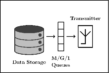
Refer to caption
(a) Data Center
Refer to caption
(b) Entities in Data Server
Fig. 1: System Model

In this paper, we consider distributed erasure-coded storage systems in wireless networks where each server is equipped with a multi-antenna base-station that is capable of wireless transmissions. Specifically, we formulate the stochastic optimization problem to find an optimal scheduling policy that maximizes users’ quality of service (QoS) while adhering to queuing delay and other deterministic constraints. Since the file transfer medium is considered wireless, we can no longer assume exponential service time distributions due to the random fading channels between user and data center. However, the classical approach is not suited due to the difficulty in evaluating closed form expressions for first and second order moments of service times with the presence of exogenous variables [13]. Recently, the authors in [14] have considered the design of queuing systems from a stochastic optimization perspective where the queues have general service time distributions. By applying ideas of [14], we show that the formulated problem has at least one of the objective and constraints has non-linear function of expectations. Hence, is not solvable with the existing SGD like first-order methods as they require unbiased estimates of (sub) gradients (see [15]).

Much recent work in [16] has presented a first-order method that deals with the non-linear functions of expectations via the stochastic compositional gradient descent (SCGD) algorithm. Since finding true (sub) gradients is not possible due to the composition structure, the SCGD algorithm adopts a quasi-gradient approach by estimating the approximated (sub) gradients. Accelerated version of SCGD is later proposed in [17]. The structure of the problem is, however, considered to be unconstrained in [16, 17]. Recently, the CSCGD algorithm has been proposed in [14] to solve constrained stochastic compositional problems. Exploring the ideas from [17, 14], we propose a new algorithm that solves constrained stochastic compositional problems with a faster convergence rate.

The rest of the paper is organized as follows. Sec. II details the system model and problem formulations. The algorithm and theoretical guarantees for it are provided in Sec. III. Later, we evaluate the performance of the proposed method in Sec. IV. Finally, we conclude our paper in Sec. V.

II System Model And Problem Formulation

We consider a data center, as shown in Fig.1, with MM servers denoted by ℳ{\mathcal{M}} that are placed in an area that is populated by users with mobile devices. Each server contains a base-station of multiple antennas that serve users through wireless transmissions, and is also capable of storing data (see Fig. 1(b)). We do not consider any interference management schemes, and hence we assume all the concurrent data transmissions by servers are transmitted in orthogonal channels. There are NN trending files of current interest, which are picked out of millions and may be delivered to the users. These selected files are the most popular ones, and they earned the placement opportunity at servers. The data objects are represented as ZiZ_{i} ∀i∈{1,…,N}\forall i\in\left\{{1,...,N}\right\}. Users can request any of these popular NN files from the data center.

II-A Coding

Each file ZiZ_{i} is divided into kik_{i} number of fixed-size chunks and then encoded using (ni,ki)(n_{i},k_{i}) Maximum Distance Separable (MDS) erasure code to generate nin_{i} distinct chunks for a file. These coded chunks are denoted as Ci(1),…,Ci(ni)C_{i}^{(1)},...,C_{i}^{(n_{i})}. The encoded chunks are stored in distinct nin_{i} servers for delivery. The servers that store the chunks corresponding to the file ii are denoted by a set 𝒮i{\mathcal{S}}_{i} such that 𝒮i⊂ℳ{\mathcal{S}}_{i}\subset{\mathcal{M}}, and |𝒮i|=ni|{\mathcal{S}}_{i}|=n_{i}. A typical MDS erasure code (ni,ki)(n_{i},k_{i}) is in such a way that ni>kin_{i}>k_{i}, with the redundancy factor ni/kin_{i}/k_{i}. Hence any subset of kik_{i}-out-of-nin_{i} coded chunks can reconstruct the original file. For example, a simple replication of a file at nn servers is nothing but using (n,1)(n,1) erasure code. We assume a centralized system that knows file placement information and schedules all the user requests to different servers. Hence, when a file is requested, the request goes to a set 𝒜i{\mathcal{A}}_{i} storage nodes where 𝒜i⊂𝒮i{\mathcal{A}}_{i}\subset{\mathcal{S}}_{i}, and |𝒜i|=ki|{\mathcal{A}}_{i}|=k_{i}. Each server maintains a FIFO queue to serve the users, as shown in Fig.1(b). When a file ii is requested, all the chunks for other file requests have not yet been served are waiting.

II-B Policy

The central system distributes the users’ requests based on the file availabilities. It has to pick the optimal choice out of many options to reduce the latency to schedule a request of file ii to the kik_{i} server. We use the Probabilistic Scheduling policy as proposed in [11] That allows the choice of every possible subset of kik_{i} nodes with a certain probability. Once a request for a file ii arrives, the central system randomly distributes the kik_{i} chunk requests to a set of nodes 𝒜i{\mathcal{A}}_{i} with predetermined probabilities P⁡(𝒜i)P({\mathcal{A}}_{i}). Then each server maintains a local queue containing all the chunk requests to finally be transmitted by the base-station. According to the Probabilistic scheduling policy, the feasible probabilities P⁡(𝒜i)P({\mathcal{A}}_{i}) exist when the following conditions are satisfied.

∑j=1mπi​j=ki​∀i​πi​j=0​ If ​j∉𝒮i,\displaystyle\sum_{j=1}^{m}\pi_{ij}=k_{i}\forall i\hskip 5.69054pt\pi_{ij}=0\text{ If }j\notin{\mathcal{S}}_{i}, (1)

where πi​j\pi_{ij} is the conditional probability of selecting the node jj for the request ii.

When we consider a simple case where only a file is placed in the system, ideally, in that case, the servers with which more users have good channels need to be scheduled. In other words, the probabilities of choosing such servers are high. The current setting however, is much more complicated. Although the files are more popular in the current scenario, the demographic preferences are unknown at this stage. For example, users that reside at various geographical locations may have different priorities towards these files. Hence to reduce the latency, we try to incorporate all of these scenarios while formulating the problem.

II-C Queuing Model

We assume the file requests follow the Poisson process with a known rate of λi\lambda_{i}. We can think of these rates λi\lambda_{i} as file popularities. Hence the arrival of chunk requests at node jj follow the Poisson with rate Λj=∑iλi​πi​j\Lambda_{j}=\sum_{i}\lambda_{i}\pi_{ij}. The chunk service time distribution is unknown and is subject to the fading channel’s random behavior, thus making the queuing models M/G/1. Let ξi​j\xi_{ij} represents the channel constant corresponding to the user who requested file ii, and pjp_{j} is the power allocated to the transmissions from the node jj. If the length of coded packet Ci𝒮iC_{i}^{{\mathcal{S}}_{i}} is LL, then the random service time XjX_{j} for the packets that leave from node jj can be written as

Xj=Lbj​(pj,ξi​j)​with probability​πi​j​λiΛj​∀i,\displaystyle X_{j}=\frac{L}{b_{j}(p_{j},\xi_{ij})}\hskip 8.53581pt\text{with probability}\hskip 8.53581pt\frac{\pi_{ij}\lambda_{i}}{\Lambda_{j}}\hskip 5.69054pt\forall i,

where bj​(pj,ξi​j)=Bj​log⁡(1+pj​ξi​j)b_{j}(p_{j},\xi_{ij})=B_{j}\log(1+p_{j}\xi_{ij}) is Shannon’s capacity, and BjB_{j} is the bandwidth of the channel. Now the first-order moment for service time can be found as

𝔼⁡[Xj]\displaystyle{\mathbb{E}}\left[{{X_{j}}}\right] =𝔼[𝔼[Xj|ξ]]\displaystyle={\mathbb{E}}\left[{{{\mathbb{E}}\left[{{X_{j}\lvert\xi}}\right]}}\right]
=L​𝔼ξ​[∑iNπi​j​λiΛj​bj​(pj,ξi​j)]\displaystyle=L{\mathbb{E}}_{{\xi}}\left[{{\sum_{i}^{N}\frac{\pi_{ij}\lambda_{i}}{\Lambda_{j}b_{j}(p_{j},\xi_{ij})}}}\right]
=L​∑iNπi​j​λiΛj​𝔼ξ​[1bj​(pj,ξi​j)]\displaystyle=L\sum_{i}^{N}\frac{\pi_{ij}\lambda_{i}}{\Lambda_{j}}{\mathbb{E}}_{{\xi}}\left[{{\frac{1}{b_{j}(p_{j},\xi_{ij})}}}\right]

where 𝔼ξ[.]{\mathbb{E}}_{{\xi}}\left[{{.}}\right] is expectation w.r.t to the only random variable 𝝃\mathbf{\xi}. Similarly, we can also find second-order moment as

𝔼⁡[Xj2]=L2​∑iNπi​j​λiΛj​𝔼ξ​[1bj2​(pj,ξi​j)]\displaystyle{\mathbb{E}}\left[{{X_{j}^{2}}}\right]=L^{2}\sum_{i}^{N}\frac{\pi_{ij}\lambda_{i}}{\Lambda_{j}}{\mathbb{E}}_{{\xi}}\left[{{\frac{1}{b^{2}_{j}(p_{j},\xi_{ij})}}}\right]

Now the average queuing delay can be calculated using the Pollaczek-Khinchin (P-K) formula as

Wj​(pj,πi​j)\displaystyle W_{j}(p_{j},\pi_{ij}) =Λj​𝔼​[Xj2]2​(1−Λj​𝔼​[Xj])\displaystyle=\frac{\Lambda_{j}{\mathbb{E}}\left[{{X_{j}^{2}}}\right]}{2(1-\Lambda_{j}{\mathbb{E}}\left[{{X_{j}}}\right])}
=L2​∑iNπi​j​λi​𝔼ξ​[1bj2​(pj,ξi​j)]2​(1−L​∑iNπi​j​λi​𝔼ξ​[1bj​(pj,ξi​j)]).\displaystyle=\frac{L^{2}\sum_{i}^{N}\pi_{ij}\lambda_{i}{\mathbb{E}}_{{\xi}}\left[{{\frac{1}{b^{2}_{j}(p_{j},\xi_{ij})}}}\right]}{2\left({1-L\sum_{i}^{N}\pi_{ij}\lambda_{i}{\mathbb{E}}_{{\xi}}\left[{{\frac{1}{b_{j}(p_{j},\xi_{ij})}}}\right]}\right)}. (2)

The complicated looking expression in (2) restricts from finding closed form for any known distributions of channel constants {ξi​j}\{\xi_{ij}\}.

II-D Problem Formulation

By assuming the information of file placement in servers is known, we formulate the problem to obtain an optimal policy that enhances the QoS of users with the following utility function

U⁡(𝐩)=∑j=1Mψ⁡(𝔼⁡[∑ibj​(pj,ξi​j)]),\displaystyle U({\mathbf{p}})=\sum_{j=1}^{M}\psi\left({{\mathbb{E}}\left[{{\sum_{i}b_{j}(p_{j},\xi_{ij})}}\right]}\right), (3)

where ψ(.)\psi(.) is any function that include such as linear, log utility functions. A simple observation tells us that the function in (3) is convex. By imposing constraints on queuing delay, the problem finally can be written as

max𝐩,Π\displaystyle\max_{{\mathbf{p}},\Pi} U⁡(𝐩)\displaystyle~U({\mathbf{p}}) (4a)
s.t Wj(pj,πi​j)≤Dj ∀j\displaystyle~W_{j}(p_{j},\pi_{ij})\leq D_{j}\text{ }\forall j (4b)
∑j=1Mpj≤P, (1).\displaystyle\sum_{j=1}^{M}p_{j}\leq P,\text{ }\eqref{polfea}. (4c)

The objective in (4a), and constraint in (4b) functions are stochastic in nature while the constraints in (4c) are deterministic which are simpler to project onto. The collection of all the random variables {ξi​j}\left\{{\xi_{ij}}\right\} is represented as 𝝃\mathbf{\xi}. The goal is to solve the above problem in online fashion using independent realizations 𝝃1\text{\boldmath$\mathbf{\xi}$}_{1}, 𝝃2\text{\boldmath$\mathbf{\xi}$}_{2}, ... that are revealed sequentially. The constraints in (4b) are expressed as non-linear functions of sample probabilities. Hence, the existing first-order methods do not apply here due to unbiased gradient estimates’ requirement to objective and constraint functions. The constraints in (4b) are convex functions (see [14, Appendix C]) thus making the whole problem in (4) convex. To the best of our knowledge, optimizing QoS in erasure-coded wireless data centers has not been considered in the existing literature. Algorithmic details to solve (4), and the theoretical convergence guarantees for it are provided in the subsequent section.

III Accelerated Stochastic Compositional Gradient Descent for Constrained Problems

Consider the more general constrained stochastic optimization problem

𝐱⋆=arg\displaystyle{\mathbf{x}}^{\star}=\arg min𝐱∈𝒳⁡f⁡(𝔼⁡[𝐠⁡(𝐱,𝝃)])+R⁡(𝐱)\displaystyle\min_{{\mathbf{x}}\in{\mathcal{X}}}~f({\mathbb{E}}\left[{{{\mathbf{g}}({\mathbf{x}},\text{\boldmath$\mathbf{\xi}$})}}\right])+R({\mathbf{x}})
s.t. ​𝐪​(𝔼⁡[𝐡⁡(𝐱,𝝃)])≤𝟎\displaystyle\text{s.t. }\hskip 5.69054pt{\mathbf{q}}({\mathbb{E}}\left[{{{\mathbf{h}}({\mathbf{x}},\text{\boldmath$\mathbf{\xi}$})}}\right])\leq{\mathbf{0}} (𝒫\mathcal{P})

where the expectation is taken with respect to 𝝃\mathbf{\xi}. Here, f:ℝm→ℝf:{\mathbb{R}}^{m}\rightarrow{\mathbb{R}}, 𝐠:ℝn×ℝk→ℝm{\mathbf{g}}:{\mathbb{R}}^{n}\times{\mathbb{R}}^{k}\rightarrow{\mathbb{R}}^{m}, 𝐡:ℝn×ℝk→ℝd{\mathbf{h}}:{\mathbb{R}}^{n}\times{\mathbb{R}}^{k}\rightarrow{\mathbb{R}}^{d}, and 𝐪:ℝd→ℝJ{\mathbf{q}}:{\mathbb{R}}^{d}\rightarrow{\mathbb{R}}^{J} are continuous functions. The penalty function R⁡(𝐱):ℝn→ℝ∪{+∞}R({\mathbf{x}}):{\mathbb{R}}^{n}\rightarrow{\mathbb{R}}\cup\left\{{+\infty}\right\} is an extended real-valued closed convex function which is allowed to be non-smooth. The problem can have simple deterministic constraints as in (4c) which can be added in R⁡(𝐱)R({\mathbf{x}}). It can be easily verified that the problem formulated in (4) is a spacial case of (III). Since the distribution of 𝝃\mathbf{\xi} is unknown, the expectations appearing in (III) cannot be evaluated in closed-form. Motivated by classical stochastic approximation methods, the goal is to solve (III) in an online fashion using only independent realizations 𝝃1\text{\boldmath$\mathbf{\xi}$}_{1}, 𝝃2\text{\boldmath$\mathbf{\xi}$}_{2}, …\ldots that are revealed sequentially. This section details the proposed algorithm for solving (III) and provides the corresponding convergence rates. For the sake of brevity, we define F⁡(𝐱):=f⁡(𝔼⁡[𝐠⁡(𝐱,𝝃)])F({\mathbf{x}}):=f({\mathbb{E}}\left[{{{\mathbf{g}}({\mathbf{x}},\text{\boldmath$\mathbf{\xi}$})}}\right]), 𝐐⁡(𝐱):=𝐪⁡(𝔼⁡[𝐡⁡(𝐱,𝝃)]){\mathbf{Q}}({\mathbf{x}}):={\mathbf{q}}({\mathbb{E}}\left[{{{\mathbf{h}}({\mathbf{x}},\text{\boldmath$\mathbf{\xi}$})}}\right]).

III-A Assumptions

We begin with discussing the necessary assumptions on the functions ff, 𝐠{\mathbf{g}}, qq and 𝐡{\mathbf{h}}. All functions ff, 𝐪{\mathbf{q}}, 𝐠{\mathbf{g}}, 𝐡{\mathbf{h}} are continuously differentiable. Consequently, the gradients of the objective and constraint functions are well-defined, with The problem (III) is a convex optimization problem and the set 𝒳{\mathcal{X}} is closed and compact, i.e., sup𝐱,𝐱′∈𝒳‖𝐱−𝐱′‖2≤Dx<∞\sup_{{\mathbf{x}},{\mathbf{x}}^{\prime}\in{\mathcal{X}}}\left\|{\mathbf{x}}-{\mathbf{x}}^{\prime}\right\|^{2}\leq D_{x}<\infty. The random variables 𝝃1,𝝃2,…\text{\boldmath$\mathbf{\xi}$}_{1},\text{\boldmath$\mathbf{\xi}$}_{2},... are independent and identically distributed. The functions 𝐠{\mathbf{g}}, 𝐡{\mathbf{h}} are Lipschitz continuous in expectation and have bounded second order moments. The functions ff, 𝐪{\mathbf{q}} are smooth and have bounded gradients. The functions FF, 𝐐{\mathbf{Q}}, and the inner functions 𝐠{\mathbf{g}}, 𝐡{\mathbf{h}} are smooth.

III-B Proposed Algorithm

Algorithm 1 Accelerated Constrained Stochastic Compositional Proximal Gradient (ACSCPG)
1:  Input: 𝐱1∈ℝn{\mathbf{x}}_{1}\in\mathbb{R}^{n} step sizes αt,βt,δt⊂(0,1]\alpha_{t},\beta_{t},\delta_{t}\subset(0,1].
2:  Initialize 𝐲1=𝐳1=0{\mathbf{y}}_{1}={\mathbf{z}}_{1}=0, 𝐰1=𝐱1{\mathbf{w}}_{1}={\mathbf{x}}_{1}.
3:  for t=1,2,…t=1,2,...
4:    Observe the random variable 𝝃t\text{\boldmath$\mathbf{\xi}$}_{t}, and update 𝐱t+1{\mathbf{x}}_{t+1}
=proxαtR(.){𝐱t−αt∇𝐠(𝐱t,𝝃t)∇f(𝐲t)\displaystyle={\text{prox}}_{\alpha_{t}R(.)}\bigg\{{\mathbf{x}}_{t}-\alpha_{t}{\nabla}{\mathbf{g}}({\mathbf{x}}_{t},\text{\boldmath$\mathbf{\xi}$}_{t}){\nabla}f({\mathbf{y}}_{t})
−δt∇𝐡(𝐱t,𝝃t)∇𝐪(𝐳t)∇ℓ(𝐪(𝐳t))}\displaystyle-\delta_{t}{\nabla}{\mathbf{h}}({\mathbf{x}}_{t},\text{\boldmath$\mathbf{\xi}$}_{t}){\nabla}{\mathbf{q}}({\mathbf{z}}_{t}){\nabla}\ell({\mathbf{q}}({\mathbf{z}}_{t}))\bigg\} (5)
5:    Observe the random variable 𝝃t+1\text{\boldmath$\mathbf{\xi}$}_{t+1}, and update the axillary iterates as
𝐰t+1\displaystyle{\mathbf{w}}_{t+1} =(1−1βt)​𝐱t+1βt​𝐱t+1,\displaystyle=\left({1-\frac{1}{\beta_{t}}}\right){\mathbf{x}}_{t}+\frac{1}{\beta_{t}}{\mathbf{x}}_{t+1}, (6)
𝐲t+1\displaystyle{\mathbf{y}}_{t+1} =(1−βt)​𝐲t+βt​𝐠​(𝐰t+1,𝝃t+1),\displaystyle=\left({1-\beta_{t}}\right){\mathbf{y}}_{t}+\beta_{t}{\mathbf{g}}\left({{\mathbf{w}}_{t+1},\text{\boldmath$\mathbf{\xi}$}_{t+1}}\right),
𝐳t+1\displaystyle{\mathbf{z}}_{t+1} =(1−βt)​𝐳t+βt​𝐡​(𝐰t+1,𝝃t+1)\displaystyle=\left({1-\beta_{t}}\right){\mathbf{z}}_{t}+\beta_{t}{\mathbf{h}}\left({{\mathbf{w}}_{t+1},\text{\boldmath$\mathbf{\xi}$}_{t+1}}\right) (7)
6:  end
7:  Output: 𝐱^=2T​∑t=T/2T𝐱t+1{\hat{{\mathbf{x}}}}=\frac{2}{T}\sum_{t=T/2}^{T}{\mathbf{x}}_{t+1}.

Similar to the analysis in [14], we define a smooth and convex function ℓ⁡(𝐰)=∑j=1Jℓj​(wj)\ell({\mathbf{w}})=\sum_{j=1}^{J}\ell_{j}(w_{j}) where ℓj\ell_{j} is defined as

ℓj​(x):={12​x20≤x≤CℓCℓ​x−Cℓ22x>Cℓ0x<0\displaystyle\ell_{j}(x):=\begin{cases}\tfrac{1}{2}x^{2}&0\leq x\leq C_{\ell}\\ C_{\ell}x-\frac{C_{\ell}^{2}}{2}&x>C_{\ell}\\ 0&x<0\end{cases} (8)

Gradient of the function is bounded as ∇ℓj​(x)=max⁡{x,Cℓ}{\nabla}\ell_{j}(x)=\max\{x,C_{\ell}\} for x>0x>0 and zero otherwise. The parameter ClC_{l} in our case is the upper limit of maxj⁡qj​(𝔼⁡[𝐡⁡(𝐱,𝝃)])\max_{j}q_{j}({\mathbb{E}}\left[{{{\mathbf{h}}({\mathbf{x}},\text{\boldmath$\mathbf{\xi}$})}}\right]) for any 𝐱∈𝒳{\mathbf{x}}\in{\mathcal{X}}. The penalty function that is defined in (8) helps in taking the iterate towards the descent direction of optimal function FF as well as towards the feasible region {𝐱:𝐐⁡(𝐱)≤0}\{{\mathbf{x}}:{\mathbf{Q}}({\mathbf{x}})\leq 0\}.

As proposed in [14], CSCGD algorithm carries updates towards the negative direction of the approximated gradients of both objective F⁡(𝐱)F({\mathbf{x}}), and penalty ℓ⁡(𝐐⁡(𝐱))\ell({\mathbf{Q}}({\mathbf{x}})) functions. However, In the present case, iterates are of similar except, the steps that track 𝔼⁡[𝐠⁡(𝐱⋆,ξ)]{\mathbb{E}}\left[{{{\mathbf{g}}({{\mathbf{x}}^{\star}},\xi)}}\right], and 𝔼⁡[𝐡⁡(𝐱⋆,ξ)]{\mathbb{E}}\left[{{{\mathbf{h}}({{\mathbf{x}}^{\star}},\xi)}}\right]. We introduce a new step in (6) that tracks running average of the optimal solution and is used in auxiliary variable updates as shown in (7) and that is called extrapolation-smoothing scheme which is the main reason behind the acceleration of convergence. The complete procedure is summarized Algorithm 1. Compared to the CSCGD, ACSCPG estimates the unknown quantities 𝔼⁡[𝐠⁡(𝐱,𝝃)]{\mathbb{E}}\left[{{{\mathbf{g}}({\mathbf{x}},\text{\boldmath$\mathbf{\xi}$})}}\right], 𝔼⁡[𝐡⁡(𝐱,𝝃)]{\mathbb{E}}\left[{{{\mathbf{h}}({\mathbf{x}},\text{\boldmath$\mathbf{\xi}$})}}\right] with faster rate. The updates in (6), (7) are carried out in way that the 𝐲t{\mathbf{y}}_{t}, 𝐳t{\mathbf{z}}_{t} are approximately unbiased estimates of 𝔼⁡[𝐠⁡(𝐱,𝝃)]{\mathbb{E}}\left[{{{\mathbf{g}}({\mathbf{x}},\text{\boldmath$\mathbf{\xi}$})}}\right], 𝔼⁡[𝐡⁡(𝐱,𝝃)]{\mathbb{E}}\left[{{{\mathbf{h}}({\mathbf{x}},\text{\boldmath$\mathbf{\xi}$})}}\right]. To explicitly see that, let us define the weights as

ζk(t)={βk​∏i=k+1t(1−βi) if ​t>k≥0βt if ​t=k≥0,\displaystyle\zeta_{k}^{(t)}=\begin{cases}\beta_{k}\prod_{i=k+1}^{t}\left({1-\beta_{i}}\right)&\text{ if }t>k\geq 0\\ \beta_{t}&\text{ if }t=k\geq 0,\end{cases} (9)

then we have the following relations

𝐱t+1\displaystyle{\mathbf{x}}_{t+1} =∑k=0tζk(t)​𝐰k+1,\displaystyle=\sum_{k=0}^{t}\zeta_{k}^{(t)}{\mathbf{w}}_{k+1},
𝐲t+1\displaystyle{\mathbf{y}}_{t+1} =∑k=0tζk(t)​𝐠​(𝐰k+1,𝝃k+1),\displaystyle=\sum_{k=0}^{t}\zeta_{k}^{(t)}{\mathbf{g}}({\mathbf{w}}_{k+1},\text{\boldmath$\mathbf{\xi}$}_{k+1}),
𝐳t+1\displaystyle{\mathbf{z}}_{t+1} =∑k=0tζk(t)​𝐡​(𝐰k+1,𝝃k+1)\displaystyle=\sum_{k=0}^{t}\zeta_{k}^{(t)}{\mathbf{h}}({\mathbf{w}}_{k+1},\text{\boldmath$\mathbf{\xi}$}_{k+1})

In other words, 𝐱t+1{\mathbf{x}}_{t+1} is weighted average of {𝐰t}1t+1\{{\mathbf{w}}_{t}\}_{1}^{t+1}, and 𝐲t+1{\mathbf{y}}_{t+1}, 𝐳t+1{\mathbf{z}}_{t+1} are weighted averages of {𝐠⁡(𝐰k+1,𝝃k+1)}1t+1\{{\mathbf{g}}({\mathbf{w}}_{k+1},\text{\boldmath$\mathbf{\xi}$}_{k+1})\}_{1}^{t+1}, {𝐡⁡(𝐰k+1,𝝃k+1)}1t+1\{{\mathbf{h}}({\mathbf{w}}_{k+1},\text{\boldmath$\mathbf{\xi}$}_{k+1})\}_{1}^{t+1}. Hence as tt progresses, the estimates 𝐲t{\mathbf{y}}_{t}, 𝐳t{\mathbf{z}}_{t} reach much nearer to the unbiased gradients of inner functions.

TABLE I: Summary of bounds on optimality gap and constraint violation
Choice of constants a,b,c,d,ea,b,c,d,e Optimality gap Constraint violation
a=0.9048a=0.9048, b=0.5714b=0.5714, c=0.7143c=0.7143, d=−0.0952d=-0.0952, e=1.2607e=1.2607 𝒪(T−2/21){\mathcal{O}}\left({T^{-2/21}}\right) 𝒪(T−2/21){\mathcal{O}}\left({T^{-2/21}}\right)
a=0.8751a=0.8751, b=0.5714b=0.5714, c=0.7143c=0.7143, d=−0.1429d=-0.1429, e=1.1652e=1.1652 𝒪(T−1/7){\mathcal{O}}\left({T^{-1/7}}\right) 𝒪(T−1/14){\mathcal{O}}\left({T^{-1/14}}\right)
a=0.7143a=0.7143, b=0.5714b=0.5714, c=0.7143c=0.7143, d=−0.2857d=-0.2857, e=0.8518e=0.8518 𝒪(T−2/7){\mathcal{O}}\left({T^{-2/7}}\right) 𝒪⁡(1){\mathcal{O}}\left({1}\right)

III-C Performance Analysis

This section provides the major theoretical findings of Algorithm. 1. We begin our analysis by defining a new objective function by penalizing the constraint as

H~​(𝐱,α,δ)=f~​(𝔼​𝐠~​(𝐱,𝝃),α,δ)+R⁡(𝐱),\displaystyle\tilde{H}({\mathbf{x}},\alpha,\delta)=\tilde{f}\left({{\mathbb{E}}\tilde{{\mathbf{g}}}\left({{\mathbf{x}},\text{\boldmath$\mathbf{\xi}$}}\right),\alpha,\delta}\right)+R({\mathbf{x}}), (10)

where

f~​(y~,α,δ)=f⁡(𝐲)+δα​p​(𝐳),p⁡(𝐳)=ℓ⁡(𝐪⁡(𝐳))\displaystyle\tilde{f}(\tilde{y},\alpha,\delta)=f({\mathbf{y}})+\frac{\delta}{\alpha}p({\mathbf{z}}),\hskip 8.53581ptp({\mathbf{z}})=\ell({\mathbf{q}}({\mathbf{z}}))
𝐠~​(𝐱,𝝃)=[𝐠⁡(𝐱,𝝃),𝐡⁡(𝐱,𝝃)],𝐲~=[𝐲,𝐳].\displaystyle\tilde{{\mathbf{g}}}\left({{\mathbf{x}},\text{\boldmath$\mathbf{\xi}$}}\right)=\left[{{\mathbf{g}}\left({{\mathbf{x}},\text{\boldmath$\mathbf{\xi}$}}\right),{\mathbf{h}}\left({{\mathbf{x}},\text{\boldmath$\mathbf{\xi}$}}\right)}\right],\hskip 8.53581pt\tilde{{\mathbf{y}}}=\left[{{\mathbf{y}},{\mathbf{z}}}\right]. (11)

Since the inner function 𝐡{\mathbf{h}} is Lipschitz and has bounded gradients, It is simple to prove (see [14, Appendix A, lemma 3]) that the function p⁡(𝐳)p({\mathbf{z}}) is smooth and have bounded gradient. Note that H~​(𝐱,α,δ)\tilde{H}({\mathbf{x}},\alpha,\delta) is convex w.r.t 𝐱{\mathbf{x}}. The following theorem establishes the convergence results of Algorithm. 1.

Theorem 1.

Under all the assumptions in Sec.III-A, for the choice of constants which are selected as

αt=C​t−a,βt=Cb​t−b,δt=C​t−c,\displaystyle\alpha_{t}=Ct^{-a},\hskip 8.53581pt\beta_{t}=C_{b}t^{-b},\hskip 8.53581pt\delta_{t}=Ct^{-c},
γt=C​t−d,ηt=C​t−e,\displaystyle\gamma_{t}=Ct^{-d},\hskip 8.53581pt\eta_{t}=Ct^{-e},

where C≥0C\geq 0, Cb>2C_{b}>2, a≥ca\geq c, 0≤a≤10\leq a\leq 1, 0≤b≤10\leq b\leq 1, and 0≤c≤10\leq c\leq 1, the following result holds.

2T\displaystyle\frac{2}{T} ∑t=T/2T𝔼⁡[H⁡(𝐱^)−H⁡(𝐱⋆)]\displaystyle\sum_{t=T/2}^{T}{\mathbb{E}}\left[{{H\left({\hat{{\mathbf{x}}}}\right)-H\left({{{\mathbf{x}}^{\star}}}\right)}}\right]
≤𝒪⁡(Ta−1+Td+T4​b−4​c−d+T−b−dCLOSE\displaystyle\leq{\mathcal{O}}\bigg(T^{a-1}+T^{d}+T^{4b-4c-d}+T^{-b-d}
+T2​a+4​b−6​c−d+T2​a−b−2​c−d+T−2​a\displaystyle\hskip 2.84526pt+T^{2a+4b-6c-d}+T^{2a-b-2c-d}+T^{-2a}
OPEN+T−a−c+T−e+T2​a−2​c−e+Te−2​a)\displaystyle\hskip 2.84526pt+T^{-a-c}+T^{-e}+T^{2a-2c-e}+T^{e-2a}\bigg)
2T\displaystyle\frac{2}{T} ∑t=T/2Tmaxj⁡𝔼⁡[Qj​(𝐱^)]\displaystyle\sum_{t=T/2}^{T}\max_{j}{\mathbb{E}}\left[{{Q_{j}\left({\hat{{\mathbf{x}}}}\right)}}\right]
≤𝒪⁡(T(c−1)/2+T(d+c−a)/2+T(4​b−3​c−d−a)/2CLOSE\displaystyle\leq{\mathcal{O}}\bigg(T^{(c-1)/2}+T^{(d+c-a)/2}+T^{(4b-3c-d-a)/2}
+T(c−a−b−d)/2+T(a+4​b−5​c−d)/2+T−a\displaystyle\hskip 2.84526pt+T^{(c-a-b-d)/2}+T^{(a+4b-5c-d)/2}+T^{-a}
+T(a−b−c−d)/2+T(−3​a+c)/2+T(c−a−e)/2\displaystyle\hskip 2.84526pt+T^{(a-b-c-d)/2}+T^{(-3a+c)/2}+T^{(c-a-e)/2}
OPEN+T(a−c−e)/2+T(e−3​a+c)/2+T(c−a)/2),\displaystyle\hskip 2.84526pt+T^{(a-c-e)/2}+T^{(e-3a+c)/2}+T^{(c-a)/2}),

where H⁡(𝐱)=F⁡(𝐱)+R⁡(𝐱)H({\mathbf{x}})=F({\mathbf{x}})+R({\mathbf{x}}).

The proof is borrowed from [17, Theorem 3]. But the presence of stochastic constraints are need to be addressed separately from [14]. Specifically, first, we bound the absolute value of successive iterate difference as 𝔼⁡[‖𝐱t+1−𝐱t‖2]≤𝒪⁡(αt2+δt2){\mathbb{E}}\left[{{\left\|{\mathbf{x}}_{t+1}-{\mathbf{x}}_{t}\right\|^{2}}}\right]\leq{\mathcal{O}}(\alpha_{t}^{2}+\delta_{t}^{2}). Then we bound the difference of tracking variables and inner functions as 𝔼⁡[‖𝐲t−𝐠¯​(𝐱t)‖2]≤𝒪⁡(t−4​c+4​b+t−b){\mathbb{E}}\left[{{\left\|{\mathbf{y}}_{t}-\bar{{\mathbf{g}}}({\mathbf{x}}_{t})\right\|^{2}}}\right]\leq{\mathcal{O}}\left({t^{-4c+4b}+t^{-b}}\right) and 𝔼⁡[‖𝐳t−𝐡¯​(𝐱t)‖2]≤𝒪⁡(t−4​c+4​b+t−b){\mathbb{E}}\left[{{\left\|{\mathbf{z}}_{t}-\bar{{\mathbf{h}}}({\mathbf{x}}_{t})\right\|^{2}}}\right]\leq{\mathcal{O}}\left({t^{-4c+4b}+t^{-b}}\right). Next by deriving the bound for difference of algorithmic and optimal solutions, we prove the statement of Theorem. 1. The complete proof is deferred to Appendix A.

By carefully choosing the constants, we obtain the rates, as shown in the Table I. Results provided in Theorem 1 are clearly improved convergence rates as 𝒪(T−2/21){\mathcal{O}}\left({T^{-2/21}}\right) compared to the best known results in [14] 𝒪(T−1/12){\mathcal{O}}\left({T^{-1/12}}\right). The improvement is due to making an additional smoothness assumption condition of inner functions.

Bounds in Table I are expressed in terms of the number of iterations. The analysis excludes the per-iteration complexity, which is fixed. Aside from the reduced number of iterations to reach the optimal solution, the number of oracle calls may be more depending on the required number of queries per iteration. For example, the addition of stochastic constraints would result in requiring more gradient queries. The current approach cannot Improve the per-iteration complexity, which is the drawback of the Algorithm. 1.

IV Simulations

Refer to caption
Fig. 2: Convergence results for ACSCPG, CSCGD [14]

We consider a data center with M=10M=10 servers; each is equipped with a single antenna base-station capable of wireless file transmissions. The most trending files N=100N=100 are considered for placement and the popularities follow Zipf distribution. Specifically, the probability pkp_{k} that k−k-th most popular file is requested at a given time adheres to pk∝k−sp_{k}\propto k^{-s} where ss is the parameter that characterizes the skewness in the distribution, which is taken as 22 for the simulation. All the files are encoded using (8,4)(8,4) MDS erasure code and stored in servers, as explained in Sec. II. Bandwidth of all the channels is allocated as Bj=1MBPS ∀j=1,…,MB_{j}=1MBPS\text{ }\forall j=1,...,M. Latency constraint is imposed as each server’s queuing delay should not go beyond 55ms. Experiments are conducted in the simulated environment of a unit radius circle where all the users and servers are present. The files’ requests are received from various locations randomly distributed in a unit radius circle with uniform distribution. The wireless channel between users and the data center is considered Rayleigh. The attenuation factor due to the path-loss is considered to k0​(d/d0)−3k_{0}(d/d_{0})^{-3} with the parameters k0=d0=1k_{0}=d_{0}=1. Eight servers are placed on the circumference of a 0.5 unit radius circle separated with 45∘45^{\circ} angular difference. The remaining two servers are placed at the coordinates (−2,0)(-2,0), (2,0)(2,0), which are far away from the users.

As the first part of the experiments, Algorithm. 1 ACSCPG is run on the simulated environment to learn the policy variables {πi​j}\left\{{\pi_{ij}}\right\} and power allocations {pj}\{p_{j}\} by trying to solve the problem (4) in online manner. For the comparison, CSCGD [14] is also run, and the results are shown in Fig.2. The two plots represent the evaluation of objective function U⁡(𝐩)U({\mathbf{p}}) (QoS metric) as in (4a), and constraints violations maxj⁡(Wj​(pj,πi​j)−Dj)\max_{j}\left({W_{j}(p_{j},\pi_{i}j)-D_{j}}\right) respectively. As shown in Fig.2, the objective is maximized, while constraint violations are decreased with the number of iterations as desired. However, the proposed algorithm outperforms CSCGD in terms of convergence rate, as supported by theoretical arguments.

Policy Throughput in (12)
Equiprobable 178 kbps
Proposed 183 kbps
TABLE II: Comparison results for Equiprobable and the proposed policies

To evaluate the proposed method’s performance in wireless networks, we implement a heuristic technique called equiprobable policy that belongs to the category of probabilistic scheduling [11] for the comparison. As the name suggests, the policy variables adhere to constraints in (1) but have equal values. We consider average throughput that is obtained from the data center as a performance metric for the comparison and is calculated as

T=1M​∑j=1M1Wj​(pj,πi​j)+1∑i𝔼⁡[bj​(pj,ξi​j)].\displaystyle T=\frac{1}{M}\sum_{j=1}^{M}\frac{1}{W_{j}(p_{j},\pi_{ij})+\frac{1}{\sum_{i}{\mathbb{E}}\left[{{b_{j}(p_{j},\xi_{ij})}}\right]}}. (12)

A good policy should obtain higher throughput. Results are presented in Table.II, and the policy obtained from the proposed method outperforms the equiprobable policy by achieving higher throughput.

V Conclusion and Future Scope

This paper considers the erasure-coded data center in a wireless network. We propose a new scheduling policy that optimizes QoS while respecting strict queuing delay constraints. To solve the problem, we propose a new algorithm, ACSCPG, which is inspired by [14, 17]. Finally, we show that the proposed algorithm beats CSCGD [14] both theoretically and in a simulated environment of a data center. We also show that the policy which is obtained from the proposed approach outperforms a heuristic one called equiprobable policy.

Apart from the benefit of rate improvements, the proposed algorithm incurs more cost per iteration with the current application. In other words, the algorithm requires approximately M+N​JM+NJ number of gradient queries in each iteration. The number M+N​JM+NJ may be much large in practice. We look for distributed versions of the current algorithm to reduce the complexity per iteration in our future works. Another interesting direction is to analyze the algorithm by considering more practical scenarios in the wireless network, such as the server nodes’ mobility.

Appendix A Proof of Theorem 1

Before proving the main result, we first derive some preliminary results.

Lemma 1.

The updates in (5) yields

𝔼⁡[‖𝐱t+1−𝐱t‖2]≤𝒪⁡(αt2+δt2).\displaystyle{\mathbb{E}}\left[{{\left\|{\mathbf{x}}_{t+1}-{\mathbf{x}}_{t}\right\|^{2}}}\right]\leq{\mathcal{O}}(\alpha_{t}^{2}+\delta_{t}^{2}). (13)

for all t≥1t\geq 1.

Proof:

From Algorithm 1

𝐱t+1=proxαtR(.)\displaystyle{\mathbf{x}}_{t+1}={\text{prox}}_{\alpha_{t}R(.)} {𝐱t−αt∇𝐠(𝐱t,𝝃t)∇f(𝐲t)\displaystyle\Big\{{\mathbf{x}}_{t}-\alpha_{t}{\nabla}{\mathbf{g}}({\mathbf{x}}_{t},\text{\boldmath$\mathbf{\xi}$}_{t}){\nabla}f({\mathbf{y}}_{t})
−δt∇𝐡(𝐱t,𝝃t)∇p(𝐳t)}.\displaystyle-\delta_{t}{\nabla}{\mathbf{h}}({\mathbf{x}}_{t},\text{\boldmath$\mathbf{\xi}$}_{t}){\nabla}p({\mathbf{z}}_{t})\Big\}.

By the definition of proximal operation, we can write

𝐱t+1=arg⁡min𝐱⁡12\displaystyle{\mathbf{x}}_{t+1}=\arg\min_{{\mathbf{x}}}\frac{1}{2} ∥𝐱−𝐱t−αt∇𝐠(𝐱t,𝝃t)∇f(𝐲t)\displaystyle\Big\|{\mathbf{x}}-{\mathbf{x}}_{t}-\alpha_{t}{\nabla}{\mathbf{g}}({\mathbf{x}}_{t},\text{\boldmath$\mathbf{\xi}$}_{t}){\nabla}f({\mathbf{y}}_{t})
−δt∇𝐡(𝐱t,𝝃t)∇p(𝐳t)∥2+αtR(𝐱).\displaystyle-\delta_{t}{\nabla}{\mathbf{h}}({\mathbf{x}}_{t},\text{\boldmath$\mathbf{\xi}$}_{t}){\nabla}p({\mathbf{z}}_{t})\Big\|^{2}+\alpha_{t}R({\mathbf{x}}).

The optimality condition suggests,

𝐱t+1−𝐱t=αt∇𝐠(𝐱t,𝝃t)∇f(𝐲t)\displaystyle{\mathbf{x}}_{t+1}-{\mathbf{x}}_{t}=\alpha_{t}{\nabla}{\mathbf{g}}({\mathbf{x}}_{t},\text{\boldmath$\mathbf{\xi}$}_{t}){\nabla}f({\mathbf{y}}_{t}) −δt∇𝐡(𝐱t,𝝃t)∇p(𝐳t)\displaystyle-\delta_{t}{\nabla}{\mathbf{h}}({\mathbf{x}}_{t},\text{\boldmath$\mathbf{\xi}$}_{t}){\nabla}p({\mathbf{z}}_{t})
+αt​𝐬t+1,\displaystyle+\alpha_{t}{\mathbf{s}}_{t+1},

where 𝐬t+1=∂R⁡(𝐱t+1){\mathbf{s}}_{t+1}=\partial R({\mathbf{x}}_{t+1}) norm of which is bounded. Hence,

‖𝐱t+1−𝐱t‖\displaystyle\left\|{\mathbf{x}}_{t+1}-{\mathbf{x}}_{t}\right\| ≤αt‖∇𝐠(𝐱t,𝝃t)∇f(𝐲t)‖\displaystyle\leq\alpha_{t}\left\|{\nabla}{\mathbf{g}}({\mathbf{x}}_{t},\text{\boldmath$\mathbf{\xi}$}_{t}){\nabla}f({\mathbf{y}}_{t})\right\|
+δt‖∇𝐡(𝐱t,𝝃t)∇p(𝐳t)‖+αt‖𝐬t+1‖\displaystyle\hskip 14.22636pt+\delta_{t}\left\|{\nabla}{\mathbf{h}}({\mathbf{x}}_{t},\text{\boldmath$\mathbf{\xi}$}_{t}){\nabla}p({\mathbf{z}}_{t})\right\|+\alpha_{t}\left\|{\mathbf{s}}_{t+1}\right\|
≤𝒪⁡(αt+δt).\displaystyle\leq{\mathcal{O}}(\alpha_{t}+\delta_{t}).

∎

Lemma 2.

Given two sequences of positive scalars {st}t=1∞\{s_{t}\}_{t=1}^{\infty}, and {ϕt}t=1∞\{\phi_{t}\}_{t=1}^{\infty} satisfying

sk+1≤(1−ϕt+C1​ϕt2)​sk+C2​t−a+C3​t−c,\displaystyle s_{k+1}\leq\left({1-\phi_{t}+C_{1}\phi_{t}^{2}}\right)s_{k}+C_{2}t^{-a}+C_{3}t^{-c},

where C1≥0C_{1}\geq 0, C2≥0C_{2}\geq 0, C3≥0C_{3}\geq 0, and a≥0a\geq 0 c≥0c\geq 0. The definition ϕt=C4​t−b\phi_{t}=C_{4}t^{-b}, where b∈(0,1]b\in(0,1], and C4>2C_{4}>2, then for any tt the sequence is bounded as

sk≤D​t−d,\displaystyle s_{k}\leq Dt^{-d},

Where DD is

maxt≤(C1​C42)1/b+1sttc+C2+C3C4−2, d=min(a−b,c−b).\displaystyle\max_{t\leq(C_{1}C_{4}^{2})^{1/b}+1}s_{t}t^{c}+\frac{C_{2}+C_{3}}{C_{4}-2},\text{ }d=\min(a-b,c-b).
Proof:

This result can be proved by induction. From the definitions it is clear that bound holds for any t≤(C1​C42)1/bt\leq(C_{1}C_{4}^{2})^{1/b}. Now assume for any t>(C1​C42)1/bt>(C_{1}C_{4}^{2})^{1/b}, st≤D​t−ds_{t}\leq Dt^{-d}. Hence we have to prove st+1≤D​(t+1)−ds_{t+1}\leq D(t+1)^{-d}.

st+1\displaystyle s_{t+1} ≤(1−ϕt+C1​ϕt2)​sk+C2​t−a+C3​t−c\displaystyle\leq\left({1-\phi_{t}+C_{1}\phi_{t}^{2}}\right)s_{k}+C_{2}t^{-a}+C_{3}t^{-c}
≤D​t−d−D​C4​t−b−d+D​C1​C42​t−2​b−d+C2​t−a\displaystyle\leq Dt^{-d}-DC_{4}t^{-b-d}+DC_{1}C_{4}^{2}t^{-2b-d}+C_{2}t^{-a}
+C3​t−c.\displaystyle\hskip 14.22636pt+C_{3}t^{-c}.

From the convexity of the function f⁡(t)=t−df(t)=t^{-d}, we can write

(t+1)−d−t−d≥−d​t−d−1.\displaystyle(t+1)^{-d}-t^{-d}\geq-dt^{-d-1}.

To prove the result we need to prove following two steps.

Δ\displaystyle\Delta =(t+1)−d−t−d+C4​t−b−d−C1​C42​t−2​b−d>0,\displaystyle=(t+1)^{-d}-t^{-d}+C_{4}t^{-b-d}-C_{1}C_{4}^{2}t^{-2b-d}>0,
D\displaystyle D ≥C2​t−a+C3​t−cΔ.\displaystyle\geq\frac{C_{2}t^{-a}+C_{3}t^{-c}}{\Delta}.

Hence we follow

Δ\displaystyle\Delta ≥−d​t−d−1+C4​t−b−d−C1​C42​t−2​b−d\displaystyle\geq-dt^{-d-1}+C_{4}t^{-b-d}-C_{1}C_{4}^{2}t^{-2b-d}
≥(C4−2)​t−b−d>0.\displaystyle\geq(C_{4}-2)t^{-b-d}>0.

The second inequality follows from the fact that t>(C1​C42)1/bt>(C_{1}C_{4}^{2})^{1/b}, and b≤1b\leq 1. Finally, we consider

C2​t−a+C3​t−cΔ\displaystyle\frac{C_{2}t^{-a}+C_{3}t^{-c}}{\Delta} ≤C2C4−2​t−a+b+d+C3C4−2​t−c+b+d\displaystyle\leq\frac{C_{2}}{C_{4}-2}t^{-a+b+d}+\frac{C_{3}}{C_{4}-2}t^{-c+b+d}
≤C2+C3C4−2≤D.\displaystyle\leq\frac{C_{2}+C_{3}}{C_{4}-2}\leq D.

The second inequality follows from the condition on dd which is d=min⁡(a−b,c−b)d=\min(a-b,c-b). ∎

Lemma 3.

If we choose βt=Cb​t−b\beta_{t}=C_{b}t^{-b}, where Cb>2C_{b}>2, b∈(0,1]b\in(0,1], and αt=Ca​t−a\alpha_{t}=C_{a}t^{-a}, δt=Cc​t−c\delta_{t}=C_{c}t^{-c}, where Ca≥0C_{a}\geq 0, Cc≥0C_{c}\geq 0, and a≥ca\geq c. Under the assumptions, we have

𝔼⁡[‖𝐲t−𝐠¯​(𝐱t)‖2]\displaystyle{\mathbb{E}}\left[{{\left\|{\mathbf{y}}_{t}-\bar{{\mathbf{g}}}({\mathbf{x}}_{t})\right\|^{2}}}\right] ≤𝒪⁡(t−4​c+4​b+t−b),\displaystyle\leq{\mathcal{O}}\left({t^{-4c+4b}+t^{-b}}\right),
𝔼⁡[‖𝐳t−𝐡¯​(𝐱t)‖2]\displaystyle{\mathbb{E}}\left[{{\left\|{\mathbf{z}}_{t}-\bar{{\mathbf{h}}}({\mathbf{x}}_{t})\right\|^{2}}}\right] ≤𝒪⁡(t−4​c+4​b+t−b).\displaystyle\leq{\mathcal{O}}\left({t^{-4c+4b}+t^{-b}}\right).
Proof:

We define,

mt+1\displaystyle m_{t+1} =∑k=0tζk(t)​‖𝐱t+1−𝐰k+1‖2\displaystyle=\sum_{k=0}^{t}\zeta_{k}^{(t)}\left\|{\mathbf{x}}_{t+1}-{\mathbf{w}}_{k+1}\right\|^{2}
nt+1\displaystyle n_{t+1} =‖∑k=0tζk(t)​(𝐠k+1​(𝐰k+1)−𝐠¯​(𝐰k+1))‖\displaystyle=\left\|\sum_{k=0}^{t}\zeta_{k}^{(t)}\left({{\mathbf{g}}_{k+1}({\mathbf{w}}_{k+1})-\bar{{\mathbf{g}}}({\mathbf{w}}_{k+1})}\right)\right\|

From [17, Lemma 7], we have

‖𝐲t−𝐠¯​(𝐱t)‖2≤Lg2​mt2+2​nt2,\displaystyle\left\|{\mathbf{y}}_{t}-\bar{{\mathbf{g}}}({\mathbf{x}}_{t})\right\|^{2}\leq L_{g}^{2}m_{t}^{2}+2n_{t}^{2},

and

qt+1\displaystyle q_{t+1} ≤(1−βt)​qk+4βt​‖𝐱t+1−𝐱t‖2\displaystyle\leq(1-\beta_{t})q_{k}+\frac{4}{\beta_{t}}\left\|{\mathbf{x}}_{t+1}-{\mathbf{x}}_{t}\right\|^{2}
≤(1−βt)​qk+𝒪⁡(t−2​a+b+t−2​c+b)\displaystyle\leq(1-\beta_{t})q_{k}+{\mathcal{O}}\left({t^{-2a+b}+t^{-2c+b}}\right)

From Lemma. 2, we can conclude qk≤𝒪⁡(t−2​c+2​b)q_{k}\leq{\mathcal{O}}(t^{-2c+2b}). Similarly from the [17, Lemme 7], we have

mt+1\displaystyle m_{t+1} ≤(1−βt)​mt+βt​qk+2βt​‖𝐱t+1−𝐱t‖2\displaystyle\leq(1-\beta_{t})m_{t}+\beta_{t}q_{k}+\frac{2}{\beta_{t}}\left\|{\mathbf{x}}_{t+1}-{\mathbf{x}}_{t}\right\|^{2}
≤(1−βt)​mt+𝒪⁡(t−2​c+b+t−2​a+b+t−2​c+b)\displaystyle\leq(1-\beta_{t})m_{t}+{\mathcal{O}}\left({t^{-2c+b}+t^{-2a+b}+t^{-2c+b}}\right)
≤(1−βt)​mt+𝒪⁡(t−2​c+b+t−2​a+b).\displaystyle\leq(1-\beta_{t})m_{t}+{\mathcal{O}}\left({t^{-2c+b}+t^{-2a+b}}\right).

Hence we have mt≤𝒪⁡(t−2​c+2​b)m_{t}\leq{\mathcal{O}}(t^{-2c+2b}). Again from the Lemma 7 in [17] we have

𝔼⁡[nt+12]≤(1−2​βt+βt2)​𝔼​[nt2]+𝒪⁡(1)​βt2.\displaystyle{\mathbb{E}}\left[{{n_{t+1}^{2}}}\right]\leq\left({1-2\beta_{t}+\beta_{t}^{2}}\right){\mathbb{E}}\left[{{n_{t}^{2}}}\right]+{\mathcal{O}}(1)\beta_{t}^{2}.

From the Lemma. 2, we have 𝔼⁡[nt2]≤𝒪⁡(t−b){\mathbb{E}}\left[{{n_{t}^{2}}}\right]\leq{\mathcal{O}}(t^{-b}). Hence we conclude

𝔼⁡[‖𝐲t−𝐠¯​(𝐱t)‖2]≤𝒪⁡(t−4​c+4​b+t−b).\displaystyle{\mathbb{E}}\left[{{\left\|{\mathbf{y}}_{t}-\bar{{\mathbf{g}}}({\mathbf{x}}_{t})\right\|^{2}}}\right]\leq{\mathcal{O}}\left({t^{-4c+4b}+t^{-b}}\right).

Similarly, we can also prove the other result. ∎

We have proved all the preliminary results. Now we prove the crucial result before discussing the convergence analysis.

Lemma 4.

Under the assumptions, for any scalers ηt\eta_{t}, and γt\gamma_{t}, the algorithmic updates yield

2\displaystyle 2 αt​𝔼​[F⁡(𝐱t+1)−F⁡(𝐱⋆)]+2​δt​𝔼​[P⁡(𝐱t+1)−P⁡(𝐱⋆)]\displaystyle\alpha_{t}{\mathbb{E}}\left[{{F\left({{\mathbf{x}}_{t+1}}\right)-F\left({{{\mathbf{x}}^{\star}}}\right)}}\right]+2\delta_{t}{\mathbb{E}}\left[{{P\left({{\mathbf{x}}_{t+1}}\right)-P\left({{{\mathbf{x}}^{\star}}}\right)}}\right]
+2​αt​𝔼​[R⁡(𝐱t+1)−R⁡(𝐱⋆)]+𝔼⁡[‖𝐱t+1−𝐱⋆‖2]\displaystyle+2\alpha_{t}{\mathbb{E}}\left[{{R({\mathbf{x}}_{t+1})-R({{\mathbf{x}}^{\star}})}}\right]+{\mathbb{E}}\left[{{\left\|{\mathbf{x}}_{t+1}-{{\mathbf{x}}^{\star}}\right\|^{2}}}\right]
≤(1+αtγt)​𝔼​[‖𝐱t−𝐱⋆‖2]+𝒪⁡(αt3+αt2​δt)\displaystyle\hskip 8.53581pt\leq\left({1+\frac{\alpha_{t}}{\gamma_{t}}}\right){\mathbb{E}}\left[{{\left\|{\mathbf{x}}_{t}-{{\mathbf{x}}^{\star}}\right\|^{2}}}\right]+{\mathcal{O}}\left({\alpha_{t}^{3}+\alpha_{t}^{2}\delta_{t}}\right)
+𝒪⁡(Lf​αt​γt)​𝔼​[‖𝐲t−𝐠¯​(𝐱t)‖2]+𝒪⁡(αt​ηt+ηt​δt2αt)\displaystyle\hskip 14.22636pt+{\mathcal{O}}\left({L_{f}\alpha_{t}\gamma_{t}}\right){\mathbb{E}}\left[{{\left\|{\mathbf{y}}_{t}-\bar{{\mathbf{g}}}({\mathbf{x}}_{t})\right\|^{2}}}\right]+{\mathcal{O}}\left({\alpha_{t}\eta_{t}+\frac{\eta_{t}\delta_{t}^{2}}{\alpha_{t}}}\right)
+𝒪⁡(αt3ηt)+𝒪⁡(Lp​γt​δt2αt)​𝔼​[‖𝐳t−𝐡¯​(𝐱t)‖2]\displaystyle\hskip 14.22636pt+{\mathcal{O}}\left({\frac{\alpha_{t}^{3}}{\eta_{t}}}\right)+{\mathcal{O}}\left({L_{p}\frac{\gamma_{t}\delta_{t}^{2}}{\alpha_{t}}}\right){\mathbb{E}}\left[{{\left\|{\mathbf{z}}_{t}-\bar{{\mathbf{h}}}({\mathbf{x}}_{t})\right\|^{2}}}\right]
Proof:

Consider ‖𝐱t+1−𝐱⋆‖2\left\|{\mathbf{x}}_{t+1}-{{\mathbf{x}}^{\star}}\right\|^{2}

=‖𝐱t+1−𝐱t+𝐱t−𝐱⋆‖2\displaystyle=\left\|{\mathbf{x}}_{t+1}-{\mathbf{x}}_{t}+{\mathbf{x}}_{t}-{{\mathbf{x}}^{\star}}\right\|^{2}
=‖𝐱t−𝐱⋆‖2−‖𝐱t+1−𝐱t‖2\displaystyle=\left\|{\mathbf{x}}_{t}-{{\mathbf{x}}^{\star}}\right\|^{2}-\left\|{\mathbf{x}}_{t+1}-{\mathbf{x}}_{t}\right\|^{2}
+2​⟨𝐱t+1−𝐱t,𝐱t+1−𝐱⋆⟩\displaystyle\hskip 8.53581pt+2\left\langle{{\mathbf{x}}_{t+1}-{\mathbf{x}}_{t}},{{\mathbf{x}}_{t+1}-{{\mathbf{x}}^{\star}}}\right\rangle
=‖𝐱t−𝐱⋆‖2−‖𝐱t+1−𝐱t‖2\displaystyle=\left\|{\mathbf{x}}_{t}-{{\mathbf{x}}^{\star}}\right\|^{2}-\left\|{\mathbf{x}}_{t+1}-{\mathbf{x}}_{t}\right\|^{2}
−2αt⟨∇𝐠~t(𝐱t)∇f~(𝐲~t,αt,δt)+𝐬t+1,𝐱t+1−𝐱⋆⟩\displaystyle\hskip 8.53581pt-2\alpha_{t}\left\langle{{\nabla}\tilde{{\mathbf{g}}}_{t}({\mathbf{x}}_{t}){\nabla}\tilde{f}\left({\tilde{{\mathbf{y}}}_{t},\alpha_{t},\delta_{t}}\right)+{\mathbf{s}}_{t+1}},{{\mathbf{x}}_{t+1}-{{\mathbf{x}}^{\star}}}\right\rangle
=‖𝐱t−𝐱⋆‖2−‖𝐱t+1−𝐱t‖2+2​αt​⟨𝐬t+1,𝐱⋆−𝐱t+1⟩\displaystyle=\left\|{\mathbf{x}}_{t}-{{\mathbf{x}}^{\star}}\right\|^{2}-\left\|{\mathbf{x}}_{t+1}-{\mathbf{x}}_{t}\right\|^{2}+2\alpha_{t}\left\langle{{\mathbf{s}}_{t+1}},{{{\mathbf{x}}^{\star}}-{\mathbf{x}}_{t+1}}\right\rangle
+2αt⟨∇𝐠~t(𝐱t)∇f~(𝐲~t,αt,δt),𝐱⋆−𝐱t+1⟩\displaystyle\hskip 8.53581pt+2\alpha_{t}\left\langle{{\nabla}\tilde{{\mathbf{g}}}_{t}({\mathbf{x}}_{t}){\nabla}\tilde{f}\left({\tilde{{\mathbf{y}}}_{t},\alpha_{t},\delta_{t}}\right)},{{{\mathbf{x}}^{\star}}-{\mathbf{x}}_{t+1}}\right\rangle
≤‖𝐱t−𝐱⋆‖2+2​αt​(R⁡(𝐱⋆)−R⁡(𝐱t+1))\displaystyle\leq\left\|{\mathbf{x}}_{t}-{{\mathbf{x}}^{\star}}\right\|^{2}+2\alpha_{t}\left({R({{\mathbf{x}}^{\star}})-R({\mathbf{x}}_{t+1})}\right)
+2αt⟨∇𝐠~t(𝐱t)∇f~(𝐲~t,αt,δt),𝐱⋆−𝐱t+1⟩\displaystyle\hskip 8.53581pt+2\alpha_{t}\left\langle{{\nabla}\tilde{{\mathbf{g}}}_{t}({\mathbf{x}}_{t}){\nabla}\tilde{f}\left({\tilde{{\mathbf{y}}}_{t},\alpha_{t},\delta_{t}}\right)},{{{\mathbf{x}}^{\star}}-{\mathbf{x}}_{t+1}}\right\rangle
=‖𝐱t−𝐱⋆‖2\displaystyle=\left\|{\mathbf{x}}_{t}-{{\mathbf{x}}^{\star}}\right\|^{2}
+2​αt​(T1+T2)+2​αt​(R⁡(𝐱⋆)−R⁡(𝐱t+1)),\displaystyle\hskip 8.53581pt+2\alpha_{t}\left({T_{1}+T_{2}}\right)+2\alpha_{t}\left({R({{\mathbf{x}}^{\star}})-R({\mathbf{x}}_{t+1})}\right),

where

T1=⟨∇F~​(𝐱t,αt,δt),𝐱⋆−𝐱t+1⟩\displaystyle T_{1}=\left\langle{{\nabla}\tilde{F}\left({{\mathbf{x}}_{t},\alpha_{t},\delta_{t}}\right)},{{{\mathbf{x}}^{\star}}-{\mathbf{x}}_{t+1}}\right\rangle
T2\displaystyle T_{2}
=⟨∇𝐠~t(𝐱t)∇f~(𝐲~t,αt,δt)−∇F~(𝐱t,αt,δt),𝐱⋆−𝐱t+1⟩.\displaystyle=\left\langle{{\nabla}\tilde{{\mathbf{g}}}_{t}({\mathbf{x}}_{t}){\nabla}\tilde{f}\left({\tilde{{\mathbf{y}}}_{t},\alpha_{t},\delta_{t}}\right)-{\nabla}\tilde{F}\left({{\mathbf{x}}_{t},\alpha_{t},\delta_{t}}\right)},{{{\mathbf{x}}^{\star}}-{\mathbf{x}}_{t+1}}\right\rangle.

The inequality follows from the fact that R⁡(𝐱)R({\mathbf{x}}) is convex. Now consider

T1\displaystyle T_{1} =⟨∇F~​(𝐱t,αt,δt),𝐱t−𝐱t+1⟩\displaystyle=\left\langle{{\nabla}\tilde{F}\left({{\mathbf{x}}_{t},\alpha_{t},\delta_{t}}\right)},{{\mathbf{x}}_{t}-{\mathbf{x}}_{t+1}}\right\rangle
+⟨∇F~​(𝐱t,αt,δt),𝐱⋆−𝐱t⟩\displaystyle\hskip 8.53581pt+\left\langle{{\nabla}\tilde{F}\left({{\mathbf{x}}_{t},\alpha_{t},\delta_{t}}\right)},{{{\mathbf{x}}^{\star}}-{\mathbf{x}}_{t}}\right\rangle
=⟨∇F​(𝐱t),𝐱t−𝐱t+1⟩+δtαt​⟨∇P​(𝐱t),𝐱t−𝐱t+1⟩\displaystyle=\left\langle{{\nabla}F\left({{\mathbf{x}}_{t}}\right)},{{\mathbf{x}}_{t}-{\mathbf{x}}_{t+1}}\right\rangle+\frac{\delta_{t}}{\alpha_{t}}\left\langle{{\nabla}P\left({{\mathbf{x}}_{t}}\right)},{{\mathbf{x}}_{t}-{\mathbf{x}}_{t+1}}\right\rangle
+⟨∇F​(𝐱t),𝐱⋆−𝐱t⟩+δtαt​⟨∇P​(𝐱t),𝐱⋆−𝐱t⟩\displaystyle\hskip 8.53581pt+\left\langle{{\nabla}F\left({{\mathbf{x}}_{t}}\right)},{{{\mathbf{x}}^{\star}}-{\mathbf{x}}_{t}}\right\rangle+\frac{\delta_{t}}{\alpha_{t}}\left\langle{{\nabla}P\left({{\mathbf{x}}_{t}}\right)},{{{\mathbf{x}}^{\star}}-{\mathbf{x}}_{t}}\right\rangle
≤F⁡(𝐱t)−F⁡(𝐱t+1)+δtαt​(P⁡(𝐱t)−P⁡(𝐱t+1))\displaystyle\leq F({\mathbf{x}}_{t})-F({\mathbf{x}}_{t+1})+\frac{\delta_{t}}{\alpha_{t}}\left({P({\mathbf{x}}_{t})-P({\mathbf{x}}_{t+1})}\right)
+12​(LF+δtαt​LP)​‖𝐱t+1−𝐱t‖2+F⁡(𝐱⋆)−F⁡(𝐱t)\displaystyle\hskip 8.53581pt+\frac{1}{2}\left({L_{F}+\frac{\delta_{t}}{\alpha_{t}}L_{P}}\right)\left\|{\mathbf{x}}_{t+1}-{\mathbf{x}}_{t}\right\|^{2}+F({{\mathbf{x}}^{\star}})-F({\mathbf{x}}_{t})
+δtαt​(P⁡(𝐱⋆)−P⁡(𝐱t))\displaystyle\hskip 8.53581pt+\frac{\delta_{t}}{\alpha_{t}}\left({P({{\mathbf{x}}^{\star}})-P({\mathbf{x}}_{t})}\right)
≤F~​(𝐱⋆,αt,δt)−F~​(𝐱t+1,αt,δt)+𝒪⁡(αt2+αt​δt).\displaystyle\leq\tilde{F}\left({{{\mathbf{x}}^{\star}},\alpha_{t},\delta_{t}}\right)-\tilde{F}\left({{\mathbf{x}}_{t+1},\alpha_{t},\delta_{t}}\right)+{\mathcal{O}}(\alpha_{t}^{2}+\alpha_{t}\delta_{t}).

Next consider T2T_{2}

=⟨∇𝐠~t(𝐱t)∇f~(𝐲~t,αt,δt)−∇F~(𝐱t,αt,δt),𝐱⋆−𝐱t+1⟩\displaystyle=\left\langle{{\nabla}\tilde{{\mathbf{g}}}_{t}({\mathbf{x}}_{t}){\nabla}\tilde{f}\left({\tilde{{\mathbf{y}}}_{t},\alpha_{t},\delta_{t}}\right)-{\nabla}\tilde{F}\left({{\mathbf{x}}_{t},\alpha_{t},\delta_{t}}\right)},{{{\mathbf{x}}^{\star}}-{\mathbf{x}}_{t+1}}\right\rangle
=T21+T22+ηt2​T23+12​ηt​‖𝐱t−𝐱t+1‖2,\displaystyle=T_{21}+T_{22}+\frac{\eta_{t}}{2}T_{23}+\frac{1}{2\eta_{t}}\left\|{\mathbf{x}}_{t}-{\mathbf{x}}_{t+1}\right\|^{2},

where

T21\displaystyle T_{21} =⟨∇F~(𝐱t,αt,δt)−∇𝐠~t(𝐱t)∇f~(𝐠~¯(𝐱t),αt,δt),\displaystyle=\Big\langle{\nabla}\tilde{F}\left({{\mathbf{x}}_{t},\alpha_{t},\delta_{t}}\right)-{\nabla}\tilde{{\mathbf{g}}}_{t}({\mathbf{x}}_{t}){\nabla}\tilde{f}\left({\bar{\tilde{{{\mathbf{g}}}}}({\mathbf{x}}_{t}),\alpha_{t},\delta_{t}}\right),
𝐱t−𝐱⋆⟩\displaystyle\hskip 17.07164pt{\mathbf{x}}_{t}-{{\mathbf{x}}^{\star}}\Big\rangle
T22\displaystyle T_{22} =⟨∇𝐠~t(𝐱t)∇f~(𝐠~¯(𝐱t),αt,δt)\displaystyle=\Big\langle{\nabla}\tilde{{\mathbf{g}}}_{t}({\mathbf{x}}_{t}){\nabla}\tilde{f}\left({\bar{\tilde{{{\mathbf{g}}}}}({\mathbf{x}}_{t}),\alpha_{t},\delta_{t}}\right)
−∇𝐠~t(𝐱t)∇f~(𝐲~t,αt,δt),𝐱t−𝐱⋆⟩\displaystyle\hskip 17.07164pt-{\nabla}\tilde{{\mathbf{g}}}_{t}({\mathbf{x}}_{t}){\nabla}\tilde{f}\left({\tilde{{\mathbf{y}}}_{t},\alpha_{t},\delta_{t}}\right),{\mathbf{x}}_{t}-{{\mathbf{x}}^{\star}}\Big\rangle
T23\displaystyle T_{23} =‖∇F~(𝐱t,αt,δt)−∇𝐠~t(𝐱t)∇f~(𝐲~t,αt,δt)‖2\displaystyle=\left\|{\nabla}\tilde{F}\left({{\mathbf{x}}_{t},\alpha_{t},\delta_{t}}\right)-{\nabla}\tilde{{\mathbf{g}}}_{t}({\mathbf{x}}_{t}){\nabla}\tilde{f}\left({\tilde{{\mathbf{y}}}_{t},\alpha_{t},\delta_{t}}\right)\right\|^{2}

We can eliminate T21T_{21}, since 𝔼​T21=0{\mathbb{E}}T_{21}=0. Hence we consider

T22\displaystyle T_{22} ≤γt2∥∇𝐠~t(𝐱t)∇f~(𝐠~¯(𝐱t),αt,δt)\displaystyle\leq\frac{\gamma_{t}}{2}\Big\|{\nabla}\tilde{{\mathbf{g}}}_{t}({\mathbf{x}}_{t}){\nabla}\tilde{f}\left({\bar{\tilde{{{\mathbf{g}}}}}({\mathbf{x}}_{t}),\alpha_{t},\delta_{t}}\right)
−∇𝐠~t(𝐱t)∇f~(𝐲~t,αt,δt)∥2+12​γt‖𝐱t−𝐱⋆‖2\displaystyle\hskip 8.53581pt-{\nabla}\tilde{{\mathbf{g}}}_{t}({\mathbf{x}}_{t}){\nabla}\tilde{f}\left({\tilde{{\mathbf{y}}}_{t},\alpha_{t},\delta_{t}}\right)\Big\|^{2}+\frac{1}{2\gamma_{t}}\left\|{\mathbf{x}}_{t}-{{\mathbf{x}}^{\star}}\right\|^{2}
≤γt‖∇𝐠t(𝐱t)∇f(𝐠¯(𝐱t))−∇𝐠t(𝐱t)∇f(𝐲t)‖2\displaystyle\leq\gamma_{t}\left\|{\nabla}{\mathbf{g}}_{t}({\mathbf{x}}_{t}){\nabla}f\left({\bar{{\mathbf{g}}}({\mathbf{x}}_{t})}\right)-{\nabla}{\mathbf{g}}_{t}({\mathbf{x}}_{t}){\nabla}f\left({{\mathbf{y}}_{t}}\right)\right\|^{2}
+γt​δt2αt2‖∇𝐡t(𝐱t)∇p(𝐡¯(𝐱t))−∇𝐡t(𝐱t)∇p(𝐳t)‖2\displaystyle\hskip 8.53581pt+\frac{\gamma_{t}\delta_{t}^{2}}{\alpha_{t}^{2}}\left\|{\nabla}{\mathbf{h}}_{t}({\mathbf{x}}_{t}){\nabla}p\left({\bar{{\mathbf{h}}}({\mathbf{x}}_{t})}\right)-{\nabla}{\mathbf{h}}_{t}({\mathbf{x}}_{t}){\nabla}p\left({{\mathbf{z}}_{t}}\right)\right\|^{2}
+12​γt​‖𝐱t−𝐱⋆‖2\displaystyle\hskip 8.53581pt+\frac{1}{2\gamma_{t}}\left\|{\mathbf{x}}_{t}-{{\mathbf{x}}^{\star}}\right\|^{2}
≤𝒪⁡(Lf​γt)​‖𝐲t−𝐠¯​(𝐱t)‖2+12​γt​‖𝐱t−𝐱⋆‖2\displaystyle\leq{\mathcal{O}}\left({L_{f}\gamma_{t}}\right)\left\|{\mathbf{y}}_{t}-\bar{{\mathbf{g}}}({\mathbf{x}}_{t})\right\|^{2}+\frac{1}{2\gamma_{t}}\left\|{\mathbf{x}}_{t}-{{\mathbf{x}}^{\star}}\right\|^{2}
+𝒪⁡(Lp​γt​δt2αt2)​‖𝐳t−𝐡¯​(𝐱t)‖2.\displaystyle\hskip 8.53581pt+{\mathcal{O}}\left({L_{p}\frac{\gamma_{t}\delta_{t}^{2}}{\alpha_{t}^{2}}}\right)\left\|{\mathbf{z}}_{t}-\bar{{\mathbf{h}}}({\mathbf{x}}_{t})\right\|^{2}.

Finally we consider

T23\displaystyle T_{23} =‖∇F~(𝐱t,αt,δt)−∇𝐠~t(𝐱t)∇f~(𝐲~t,αt,δt)‖2\displaystyle=\left\|{\nabla}\tilde{F}\left({{\mathbf{x}}_{t},\alpha_{t},\delta_{t}}\right)-{\nabla}\tilde{{\mathbf{g}}}_{t}({\mathbf{x}}_{t}){\nabla}\tilde{f}\left({\tilde{{\mathbf{y}}}_{t},\alpha_{t},\delta_{t}}\right)\right\|^{2}
=∥∇F(𝐱t)+δtαt∇P(𝐱t)−∇𝐠t(𝐱t)∇f(𝐲t)\displaystyle=\Big\|{\nabla}F\left({{\mathbf{x}}_{t}}\right)+\frac{\delta_{t}}{\alpha_{t}}{\nabla}P({\mathbf{x}}_{t})-{\nabla}{\mathbf{g}}_{t}({\mathbf{x}}_{t}){\nabla}f\left({{\mathbf{y}}_{t}}\right)
−δtαt∇𝐡t(𝐱t)∇p(𝐳t)∥2\displaystyle\hskip 8.53581pt-\frac{\delta_{t}}{\alpha_{t}}{\nabla}{\mathbf{h}}_{t}({\mathbf{x}}_{t}){\nabla}p\left({{\mathbf{z}}_{t}}\right)\Big\|^{2}
≤𝒪⁡(1+δt2αt2).\displaystyle\leq{\mathcal{O}}\left({1+\frac{\delta_{t}^{2}}{\alpha_{t}^{2}}}\right).

Now By considering all the intermediate results we conclude

𝔼⁡[‖𝐱t+1−𝐱⋆‖2]≤(1+αtγt)​𝔼​[‖𝐱t−𝐱⋆‖2]\displaystyle{\mathbb{E}}\left[{{\left\|{\mathbf{x}}_{t+1}-{{\mathbf{x}}^{\star}}\right\|^{2}}}\right]\leq\left({1+\frac{\alpha_{t}}{\gamma_{t}}}\right){\mathbb{E}}\left[{{\left\|{\mathbf{x}}_{t}-{{\mathbf{x}}^{\star}}\right\|^{2}}}\right]
+2​αt​F~​(𝐱⋆,αt,δt)−2​αt​𝔼​[F~​(𝐱t+1,αt,δt)]+𝒪⁡(αt3ηt)\displaystyle+2\alpha_{t}\tilde{F}\left({{{\mathbf{x}}^{\star}},\alpha_{t},\delta_{t}}\right)-2\alpha_{t}{\mathbb{E}}\left[{{\tilde{F}\left({{\mathbf{x}}_{t+1},\alpha_{t},\delta_{t}}\right)}}\right]+{\mathcal{O}}\left({\frac{\alpha_{t}^{3}}{\eta_{t}}}\right)
+𝒪⁡(Lf​αt​γt)​𝔼​[‖𝐲t−𝐠¯​(𝐱t)‖2]+𝒪⁡(αt​ηt+ηt​δt2αt)\displaystyle+{\mathcal{O}}\left({L_{f}\alpha_{t}\gamma_{t}}\right){\mathbb{E}}\left[{{\left\|{\mathbf{y}}_{t}-\bar{{\mathbf{g}}}({\mathbf{x}}_{t})\right\|^{2}}}\right]+{\mathcal{O}}\left({\alpha_{t}\eta_{t}+\frac{\eta_{t}\delta_{t}^{2}}{\alpha_{t}}}\right)
+𝒪⁡(Lp​γt​δt2αt)​𝔼​[‖𝐳t−𝐡¯​(𝐱t)‖2]+𝒪⁡(αt3+αt2​δt)\displaystyle+{\mathcal{O}}\left({L_{p}\frac{\gamma_{t}\delta_{t}^{2}}{\alpha_{t}}}\right){\mathbb{E}}\left[{{\left\|{\mathbf{z}}_{t}-\bar{{\mathbf{h}}}({\mathbf{x}}_{t})\right\|^{2}}}\right]+{\mathcal{O}}(\alpha_{t}^{3}+\alpha_{t}^{2}\delta_{t})
+2​αt​𝔼​[R⁡(𝐱⋆)−R⁡(𝐱t+1)].\displaystyle+2\alpha_{t}{\mathbb{E}}\left[{{R({{\mathbf{x}}^{\star}})-R({\mathbf{x}}_{t+1})}}\right].

We get the required result by interchanging the terms. ∎

Now we are ready with all the derived results, we proceed to prove the theorem. Let us denote

H⁡(𝐱)=F⁡(𝐱)+R⁡(𝐱).\displaystyle H({\mathbf{x}})=F({\mathbf{x}})+R({\mathbf{x}}).

Further we know P⁡(𝐱⋆)=0P({\mathbf{x}}^{\star})=0. Now by summing over 1,…,T1,...,T the expression of Lemma. 4, we get

∑t=T/2T(2​𝔼​[H⁡(𝐱t+1)−H⁡(𝐱⋆)]+2​δtαt​𝔼​[P⁡(𝐱t+1)])\displaystyle\sum_{t=T/2}^{T}\left({2{\mathbb{E}}\left[{{H\left({{\mathbf{x}}_{t+1}}\right)-H\left({{{\mathbf{x}}^{\star}}}\right)}}\right]+2\frac{\delta_{t}}{\alpha_{t}}{\mathbb{E}}\left[{{P\left({{\mathbf{x}}_{t+1}}\right)}}\right]}\right)
≤1αT/2​𝔼​[‖𝐱1−𝐱⋆‖2]+∑t=T/2T1γt​𝔼​[‖𝐱t−𝐱⋆‖2]\displaystyle\hskip 8.53581pt\leq\frac{1}{\alpha_{T/2}}{\mathbb{E}}\left[{{\left\|{\mathbf{x}}_{1}-{{\mathbf{x}}^{\star}}\right\|^{2}}}\right]+\sum_{t=T/2}^{T}\frac{1}{\gamma_{t}}{\mathbb{E}}\left[{{\left\|{\mathbf{x}}_{t}-{{\mathbf{x}}^{\star}}\right\|^{2}}}\right]
+∑t=T/2T𝒪(γt​δt2αt2)𝔼[‖𝐳t−𝐡¯(𝐱t)‖2]\displaystyle\hskip 14.22636pt+\sum_{t=T/2}^{T}{\mathcal{O}}\left({\frac{\gamma_{t}\delta_{t}^{2}}{\alpha_{t}^{2}}}\right){\mathbb{E}}\left[{{\left\|{\mathbf{z}}_{t}-\bar{{\mathbf{h}}}({\mathbf{x}}_{t})\right\|^{2}}}\right]
+∑t=T/2T𝒪(γt)𝔼[‖𝐲t−𝐠¯(𝐱t)‖2]\displaystyle\hskip 14.22636pt+\sum_{t=T/2}^{T}{\mathcal{O}}\left({\gamma_{t}}\right){\mathbb{E}}\left[{{\left\|{\mathbf{y}}_{t}-\bar{{\mathbf{g}}}({\mathbf{x}}_{t})\right\|^{2}}}\right]
+∑t=T/2T𝒪(αt2+αtδt+ηt+ηt​δt2αt2+αt2ηt)\displaystyle\hskip 14.22636pt+\sum_{t=T/2}^{T}{\mathcal{O}}\left({\alpha_{t}^{2}+\alpha_{t}\delta_{t}+\eta_{t}+\frac{\eta_{t}\delta_{t}^{2}}{\alpha_{t}^{2}}+\frac{\alpha_{t}^{2}}{\eta_{t}}}\right)
≤∑t=T/2T𝒪⁡(γt​δt2αt2)​𝔼​[‖𝐳t−𝐡¯​(𝐱t)‖2]+𝒪⁡(1αT/2)\displaystyle\hskip 8.53581pt\leq\sum_{t=T/2}^{T}{\mathcal{O}}\left({\frac{\gamma_{t}\delta_{t}^{2}}{\alpha_{t}^{2}}}\right){\mathbb{E}}\left[{{\left\|{\mathbf{z}}_{t}-\bar{{\mathbf{h}}}({\mathbf{x}}_{t})\right\|^{2}}}\right]+{\mathcal{O}}\left({\frac{1}{\alpha_{T/2}}}\right)
+𝒪⁡(∑t=T/2T1γt)+∑t=T/2T𝒪⁡(γt)​𝔼​[‖𝐲t−𝐠¯​(𝐱t)‖2]\displaystyle\hskip 14.22636pt+{\mathcal{O}}\left({\sum_{t=T/2}^{T}\frac{1}{\gamma_{t}}}\right)+\sum_{t=T/2}^{T}{\mathcal{O}}\left({\gamma_{t}}\right){\mathbb{E}}\left[{{\left\|{\mathbf{y}}_{t}-\bar{{\mathbf{g}}}({\mathbf{x}}_{t})\right\|^{2}}}\right]
+∑t=T/2T𝒪(αt2+αtδt+ηt+ηt​δt2αt2+αt2ηt)\displaystyle\hskip 14.22636pt+\sum_{t=T/2}^{T}{\mathcal{O}}\left({\alpha_{t}^{2}+\alpha_{t}\delta_{t}+\eta_{t}+\frac{\eta_{t}\delta_{t}^{2}}{\alpha_{t}^{2}}+\frac{\alpha_{t}^{2}}{\eta_{t}}}\right)

The second inequality follows from the fact that ‖𝐱t−𝐱⋆‖2≤𝒪⁡(1)\left\|{\mathbf{x}}_{t}-{{\mathbf{x}}^{\star}}\right\|^{2}\leq{\mathcal{O}}(1). From the results in Lemma. 3, we can write

∑t=T/2T(2​𝔼​[H⁡(𝐱t+1)−H⁡(𝐱⋆)]+2​δtαt​𝔼​[P⁡(𝐱t+1)])\displaystyle\sum_{t=T/2}^{T}\left({2{\mathbb{E}}\left[{{H\left({{\mathbf{x}}_{t+1}}\right)-H\left({{{\mathbf{x}}^{\star}}}\right)}}\right]+2\frac{\delta_{t}}{\alpha_{t}}{\mathbb{E}}\left[{{P\left({{\mathbf{x}}_{t+1}}\right)}}\right]}\right)
≤∑t=T/2T(𝒪⁡(γt)+𝒪⁡(γt​δt2αt2))​𝒪​((δtβt)4+βt)\displaystyle\hskip 8.53581pt\leq\sum_{t=T/2}^{T}\left({{\mathcal{O}}\left({\gamma_{t}}\right)+{\mathcal{O}}\left({\frac{\gamma_{t}\delta_{t}^{2}}{\alpha_{t}^{2}}}\right)}\right){\mathcal{O}}\left({\left({\frac{\delta_{t}}{\beta_{t}}}\right)^{4}+\beta_{t}}\right)
+∑t=1T𝒪(αt2+αtδt+ηt+ηt​δt2αt2+αt2ηt)\displaystyle\hskip 14.22636pt+\sum_{t=1}^{T}{\mathcal{O}}\left({\alpha_{t}^{2}+\alpha_{t}\delta_{t}+\eta_{t}+\frac{\eta_{t}\delta_{t}^{2}}{\alpha_{t}^{2}}+\frac{\alpha_{t}^{2}}{\eta_{t}}}\right)
+𝒪⁡(1αT/2)+𝒪⁡(∑t=T/2T1γt)\displaystyle\hskip 14.22636pt+{\mathcal{O}}\left({\frac{1}{\alpha_{T/2}}}\right)+{\mathcal{O}}\left({\sum_{t=T/2}^{T}\frac{1}{\gamma_{t}}}\right)
≤∑t=T/2T𝒪⁡(γt​δt4βt4+βt​γt+γt​δt6αt2​βt4+γt​δt2​βtαt2)\displaystyle\hskip 8.53581pt\leq\sum_{t=T/2}^{T}{\mathcal{O}}\left({\frac{\gamma_{t}\delta_{t}^{4}}{\beta_{t}^{4}}+\beta_{t}\gamma_{t}+\frac{\gamma_{t}\delta_{t}^{6}}{\alpha_{t}^{2}\beta_{t}^{4}}+\frac{\gamma_{t}\delta_{t}^{2}\beta_{t}}{\alpha_{t}^{2}}}\right)
+∑t=T/2T𝒪(αt2+αtδt+ηt+ηt​δt2αt2+αt2ηt)\displaystyle\hskip 14.22636pt+\sum_{t=T/2}^{T}{\mathcal{O}}\left({\alpha_{t}^{2}+\alpha_{t}\delta_{t}+\eta_{t}+\frac{\eta_{t}\delta_{t}^{2}}{\alpha_{t}^{2}}+\frac{\alpha_{t}^{2}}{\eta_{t}}}\right)
+𝒪⁡(1αT/2)+𝒪⁡(∑t=T/2T1γt)\displaystyle\hskip 14.22636pt+{\mathcal{O}}\left({\frac{1}{\alpha_{T/2}}}\right)+{\mathcal{O}}\left({\sum_{t=T/2}^{T}\frac{1}{\gamma_{t}}}\right) (14)

Now For the first result since we know P⁡(𝐱t+1)≥0P\left({{\mathbf{x}}_{t+1}}\right)\geq 0, we write

∑t=T/2T2​𝔼​[H⁡(𝐱t+1)−H⁡(𝐱⋆)]\displaystyle\sum_{t=T/2}^{T}2{\mathbb{E}}\left[{{H\left({{\mathbf{x}}_{t+1}}\right)-H\left({{{\mathbf{x}}^{\star}}}\right)}}\right]
≤∑t=T/2T𝒪⁡(γt​δt4βt4+βt​γt+γt​δt6αt2​βt4+γt​δt2​βtαt2)\displaystyle\hskip 8.53581pt\leq\sum_{t=T/2}^{T}{\mathcal{O}}\left({\frac{\gamma_{t}\delta_{t}^{4}}{\beta_{t}^{4}}+\beta_{t}\gamma_{t}+\frac{\gamma_{t}\delta_{t}^{6}}{\alpha_{t}^{2}\beta_{t}^{4}}+\frac{\gamma_{t}\delta_{t}^{2}\beta_{t}}{\alpha_{t}^{2}}}\right)
+∑t=T/2T𝒪(αt2+αtδt+ηt+ηt​δt2αt2+αt2ηt)\displaystyle\hskip 14.22636pt+\sum_{t=T/2}^{T}{\mathcal{O}}\left({\alpha_{t}^{2}+\alpha_{t}\delta_{t}+\eta_{t}+\frac{\eta_{t}\delta_{t}^{2}}{\alpha_{t}^{2}}+\frac{\alpha_{t}^{2}}{\eta_{t}}}\right)
+𝒪⁡(1αT/2)+𝒪⁡(∑t=T/2T1γt).\displaystyle\hskip 14.22636pt+{\mathcal{O}}\left({\frac{1}{\alpha_{T/2}}}\right)+{\mathcal{O}}\left({\sum_{t=T/2}^{T}\frac{1}{\gamma_{t}}}\right).

After substituting all the constants choices,

∑t=T/2T2​𝔼​[H⁡(𝐱t+1)−H⁡(𝐱⋆)]≤𝒪⁡(Ta)+𝒪⁡(∑t=T/2Ttd)\displaystyle\sum_{t=T/2}^{T}2{\mathbb{E}}\left[{{H\left({{\mathbf{x}}_{t+1}}\right)-H\left({{{\mathbf{x}}^{\star}}}\right)}}\right]\leq{\mathcal{O}}\left({T^{a}}\right)+{\mathcal{O}}\left({\sum_{t=T/2}^{T}t^{d}}\right)
+∑t=T/2T𝒪(t4​b−4​c−d+t2​a+4​b−6​c−d+t2​a−b−2​c−d\displaystyle+\sum_{t=T/2}^{T}{\mathcal{O}}\Big(t^{4b-4c-d}+t^{2a+4b-6c-d}+t^{2a-b-2c-d}
OPEN+t−b−d+t−2​a+t−a−c+t−e+t2​a−2​c−e+te−2​a)\displaystyle+t^{-b-d}+t^{-2a}+t^{-a-c}+t^{-e}+t^{2a-2c-e}+t^{e-2a}\Big)
≊𝒪⁡(Ta+Td+1+T1+4​b−4​c−d+T1−b−dCLOSE\displaystyle\approxeq{\mathcal{O}}\Big(T^{a}+T^{d+1}+T^{1+4b-4c-d}+T^{1-b-d}
+T1+2​a+4​b−6​c−d+T1+2​a−b−2​c−d+T1−2​a+T1−a−c\displaystyle+T^{1+2a+4b-6c-d}+T^{1+2a-b-2c-d}+T^{1-2a}+T^{1-a-c}
OPEN+T1−e+T1+2​a−2​c−e+T1+e−2​a).\displaystyle+T^{1-e}+T^{1+2a-2c-e}+T^{1+e-2a}\Big).

Proceeding further

2T​∑t=T/2T𝔼⁡[H⁡(𝐱t+1)−H⁡(𝐱⋆)]≤𝒪⁡(Ta−1+TdCLOSE\displaystyle\frac{2}{T}\sum_{t=T/2}^{T}{\mathbb{E}}\left[{{H\left({{\mathbf{x}}_{t+1}}\right)-H\left({{{\mathbf{x}}^{\star}}}\right)}}\right]\leq{\mathcal{O}}\Big(T^{a-1}+T^{d}
+T4​b−4​c−d+T−b−d+T2​a+4​b−6​c−d+T2​a−b−2​c−d\displaystyle\hskip 8.53581pt+T^{4b-4c-d}+T^{-b-d}+T^{2a+4b-6c-d}+T^{2a-b-2c-d}
OPEN+𝒪​T−2​a+T−a−c+T−e+T2​a−2​c−e+Te−2​a).\displaystyle\hskip 8.53581pt+{\mathcal{O}}T^{-2a}+T^{-a-c}+T^{-e}+T^{2a-2c-e}+T^{e-2a}\Big).

Hence from the convexity of HH, first result of Thm.1 is proved.

Now for the second results since we know |𝔼⁡[H⁡(𝐱t+1)−H⁡(𝐱⋆)]|≥−𝒪⁡(1)|{\mathbb{E}}\left[{{H\left({{\mathbf{x}}_{t+1}}\right)-H\left({{{\mathbf{x}}^{\star}}}\right)}}\right]|\geq-{\mathcal{O}}(1). Since αt≤δt\alpha_{t}\leq\delta_{t}, and the function PP is convex we have

T​δT/22​αT/2​𝔼​[P⁡(𝐱^)]\displaystyle\frac{T\delta_{T/2}}{2\alpha_{T/2}}{\mathbb{E}}\left[{{P\left({\hat{{\mathbf{x}}}}\right)}}\right] ≤δT/2αT/2​∑t=T/2T𝔼⁡[P⁡(𝐱t+1)]\displaystyle\leq\frac{\delta_{T/2}}{\alpha_{T/2}}\sum_{t=T/2}^{T}{\mathbb{E}}\left[{{P\left({{\mathbf{x}}_{t+1}}\right)}}\right]
≤∑t=T/2Tδtαt​𝔼​[P⁡(𝐱t+1)].\displaystyle\leq\sum_{t=T/2}^{T}\frac{\delta_{t}}{\alpha_{t}}{\mathbb{E}}\left[{{P\left({{\mathbf{x}}_{t+1}}\right)}}\right]. (15)

From the definition of function PP provided in (11), and penalty function in (8), we know P⁡(𝐱^)=∑j([Qj​(𝐱^)]+)2P(\hat{{\mathbf{x}}})=\sum_{j}\left({\left[{Q_{j}(\hat{{\mathbf{x}}})}\right]_{+}}\right)^{2} where [.]+[.]_{+} is the projection on positive orthant. Therefore the expression in (15) becomes

T​δT/22​J​αT/2​(∑j=1J[Qj​(𝐱^)]+)2\displaystyle\frac{T\delta_{T/2}}{2J\alpha_{T/2}}\left({\sum_{j=1}^{J}\left[{Q_{j}(\hat{{\mathbf{x}}})}\right]_{+}}\right)^{2} ≤T​δT/22​αT/2​∑j=1J([Qj​(𝐱^)]+)2\displaystyle\leq\frac{T\delta_{T/2}}{2\alpha_{T/2}}\sum_{j=1}^{J}\left({\left[{Q_{j}(\hat{{\mathbf{x}}})}\right]_{+}}\right)^{2}
≤∑t=T/2Tδtαt​𝔼​[P⁡(𝐱^)].\displaystyle\leq\sum_{t=T/2}^{T}\frac{\delta_{t}}{\alpha_{t}}{\mathbb{E}}\left[{{P\left({\hat{{\mathbf{x}}}}\right)}}\right]. (16)

From the expression in (14), we can write

2​δT/2αT/2​∑t=T/2T𝔼⁡[P⁡(𝐱t+1)]\displaystyle 2\frac{\delta_{T/2}}{\alpha_{T/2}}\sum_{t=T/2}^{T}{\mathbb{E}}\left[{{P\left({{\mathbf{x}}_{t+1}}\right)}}\right]
≤∑t=T/2T𝒪⁡(γt​δt4βt4+βt​γt+γt​δt6αt2​βt4+γt​δt2​βtαt2)\displaystyle\hskip 8.53581pt\leq\sum_{t=T/2}^{T}{\mathcal{O}}\left({\frac{\gamma_{t}\delta_{t}^{4}}{\beta_{t}^{4}}+\beta_{t}\gamma_{t}+\frac{\gamma_{t}\delta_{t}^{6}}{\alpha_{t}^{2}\beta_{t}^{4}}+\frac{\gamma_{t}\delta_{t}^{2}\beta_{t}}{\alpha_{t}^{2}}}\right)
+∑t=T/2T𝒪(αt2+αtδt+ηt+ηt​δt2αt2+αt2ηt)\displaystyle\hskip 14.22636pt+\sum_{t=T/2}^{T}{\mathcal{O}}\left({\alpha_{t}^{2}+\alpha_{t}\delta_{t}+\eta_{t}+\frac{\eta_{t}\delta_{t}^{2}}{\alpha_{t}^{2}}+\frac{\alpha_{t}^{2}}{\eta_{t}}}\right)
+𝒪⁡(1αT/2)+𝒪⁡(∑t=T/2T1γt)+𝒪⁡(T)\displaystyle\hskip 14.22636pt+{\mathcal{O}}\left({\frac{1}{\alpha_{T/2}}}\right)+{\mathcal{O}}\left({\sum_{t=T/2}^{T}\frac{1}{\gamma_{t}}}\right)+{\mathcal{O}}(T)
≊𝒪⁡(Ta+Td+1+T1+4​b−4​c−d+T1+2​a+4​b−6​c−dCLOSE\displaystyle\hskip 8.53581pt\approxeq{\mathcal{O}}\Big(T^{a}+T^{d+1}+T^{1+4b-4c-d}+T^{1+2a+4b-6c-d}
+T1−b−d+T1+2​a−b−2​c−d+T1−2​a+T1−a−c\displaystyle\hskip 14.22636pt+T^{1-b-d}+T^{1+2a-b-2c-d}+T^{1-2a}+T^{1-a-c}
OPEN+T1−e+T1+2​a−2​c−e+T1+e−2​a+T).\displaystyle\hskip 14.22636pt+T^{1-e}+T^{1+2a-2c-e}+T^{1+e-2a}+T\Big).

By taking δT/2/αT/2\delta_{T/2}/\alpha_{T/2} to R.H.S and dividing with TT, we can write

2T​∑t=T/2T𝔼⁡[P⁡(𝐱t+1)]\displaystyle\frac{2}{T}\sum_{t=T/2}^{T}{\mathbb{E}}\left[{{P\left({{\mathbf{x}}_{t+1}}\right)}}\right]
≤𝒪⁡(Tc−1+Td+c−a+T4​b−3​c−d−a+Tc−a−b−dCLOSE\displaystyle\hskip 8.53581pt\leq{\mathcal{O}}\Big(T^{c-1}+T^{d+c-a}+T^{4b-3c-d-a}+T^{c-a-b-d}
+Ta+4​b−5​c−d+Ta−b−c−d+T−3​a+c+T−2​a\displaystyle\hskip 14.22636pt+T^{a+4b-5c-d}+T^{a-b-c-d}+T^{-3a+c}+T^{-2a}
OPEN+Tc−a−e+Ta−c−e+Te−3​a+c+Tc−a)\displaystyle\hskip 14.22636pt+T^{c-a-e}+T^{a-c-e}+T^{e-3a+c}+T^{c-a}\Big)

From the expression in (16), we conclude the proof by saying

∑j=1J[Qj​(𝐱^)]+\displaystyle\sum_{j=1}^{J}\left[{Q_{j}(\hat{{\mathbf{x}}})}\right]_{+}
≤𝒪⁡(T(c−1)/2+T(d+c−a)/2+T(4​b−3​c−d−a)/2CLOSE\displaystyle\hskip 8.53581pt\leq{\mathcal{O}}\Big(T^{(c-1)/2}+T^{(d+c-a)/2}+T^{(4b-3c-d-a)/2}
+T(c−a−b−d)/2+T(a+4​b−5​c−d)/2+T(a−b−c−d)/2\displaystyle\hskip 14.22636pt+T^{(c-a-b-d)/2}+T^{(a+4b-5c-d)/2}+T^{(a-b-c-d)/2}
+T(−3​a+c)/2+T−a+T(c−a−e)/2+T(a−c−e)/2\displaystyle\hskip 14.22636pt+T^{(-3a+c)/2}+T^{-a}+T^{(c-a-e)/2}+T^{(a-c-e)/2}
OPEN+T(e−3​a+c)/2+T(c−a)/2).\displaystyle\hskip 14.22636pt+T^{(e-3a+c)/2}+T^{(c-a)/2}\Big).

References

  • [1] M. Asteris, D. Papailiopoulos, A. G. Dimakis, R. Vadali, S. Chen, and D. Borthakur, “Xoring elephants: Novel erasure codes for big data,” in Proc. Int. Conf. Very Large Data Bases, pp. 325–336.
  • [2] C. Huang, H. Simitci, Y. Xu, A. Ogus, B. Calder, P. Gopalan, J. Li, and S. Yekhanin, “Erasure coding in windows azure storage,” in Proc. {\{USENIX}\} Annu. Tech. Conf., 2012, pp. 1–16.
  • [3] A. Fikes, “Storage architecture and challenges,” Talk at the Google Faculty Summit, vol. 535, 2010.
  • [4] H. Weatherspoon and J. D. Kubiatowicz, “Erasure coding vs. replication: A quantitative comparison,” in Proc. Int. Workshop Peer-to-Peer Syst. New York, NY, USA: Springer-Verlag, 2002.
  • [5] A. G. Dimakis, P. B. Godfrey, Y. Wu, M. J. Wainwright, and K. Ramchandran, “Network coding for distributed storage systems,” IEEE Trans. Inf. Theory, vol. 56, no. 9, pp. 4539–4551, 2010.
  • [6] M. K. Aguilera, R. Janakiraman, and L. Xu, “Using erasure codes efficiently for storage in a distributed system,” in Proc. Intl. Conf. on DSN. IEEE, 2005, pp. 336–345.
  • [7] J. Li, “Adaptive erasure resilient coding in distributed storage,” in Proc. IEEE ICME, 2006, pp. 561–564.
  • [8] E. Schurman and J. Brutlag, “The user and business impact of server delays, additional bytes, and http chunking in web search,” in Proc. OReilly Velocity Web Perform. Oper. Conf., Jun, 2009.
  • [9] L. Huang, S. Pawar, H. Zhang, and K. Ramchandran, “Codes can reduce queueing delay in data centers,” in Proc. IEEE ISIT, 2012, pp. 2766–2770.
  • [10] G. Joshi, Y. Liu, and E. Soljanin, “On the delay-storage trade-off in content download from coded distributed storage systems,” vol. 32, no. 5, pp. 989–997, 2014.
  • [11] Y. Xiang, T. Lan, V. Aggarwal, and Y.-F. R. Chen, “Joint latency and cost optimization for erasure-coded data center storage,” IEEE/ACM Trans. Netw., vol. 24, no. 4, pp. 2443–2457, 2016.
  • [12] A. O. Al-Abbasi and V. Aggarwal, “Video streaming in distributed erasure-coded storage systems: Stall duration analysis,” IEEE/ACM Trans. Netw., vol. 26, no. 4, pp. 1921–1932, 2018.
  • [13] S. Lee, M. Han, and D. Hong, “Average snr and ergodic capacity analysis for opportunistic dfrelaying with outage over rayleigh fading channels,” IEEE Trans. Wireless Commun., vol. 8, no. 6, pp. 2807–2812, 2009.
  • [14] S. T. Thomdapu and K. Rajawat, “Optimal design of queuing systems via compositional stochastic programming,” IEEE Trans. Commun., vol. 67, no. 12, pp. 8460–8474, 2019.
  • [15] A. Benveniste, M. Métivier, and P. Priouret, Adaptive algorithms and stochastic approximations. Springer Science & Business Media, 2012, vol. 22.
  • [16] M. Wang, E. X. Fang, and H. Liu, “Stochastic compositional gradient descent: algorithms for minimizing compositions of expected-value functions,” Mathematical Programming, vol. 161, no. 1-2, pp. 419–449, 2017.
  • [17] M. Wang, J. Liu, and E. X. Fang, “Accelerating stochastic composition optimization,” The Journal of Machine Learning Research, vol. 18, no. 1, pp. 3721–3743, 2017.