Data-Driven Secondary Control of Distributed Energy Resources
Abstract
In this paper, we present a data-driven secondary controller for regulating to some desired values several variables of interest in a power system, namely, electrical frequency, voltage magnitudes at critical buses, and active power flows through critical lines. The power generation system is based on distributed energy resources (DERs) interfaced with either grid-forming (GFM) or grid-following (GFL) inverters. The secondary controller is based on online feedback optimization leveraging the learned sensitivities of the changes in the system frequency, voltage magnitudes at critical buses, and active power flows through critical lines to the changes in inverter active and reactive power setpoints. To learn the sensitivities accurately from data, the feedback optimization has a built-in mechanism for keeping the secondary control inputs persistently exciting without degrading its performance. The feedback optimization also utilizes the learned power-voltage characteristics of photovoltaic (PV) arrays to compute DC-link voltage setpoints so as to allow the PV arrays to track the power setpoints. To learn the power-voltage characteristics, we separately execute a data-driven approach that fits a concave polynomial to the collected power-voltage measurements by solving a sum-of-squares (SoS) optimization. We showcase the secondary controller using the modified IEEE- bus test system, in which conventional energy sources are replaced with inverter-interfaced DERs.
I Introduction
With the increased installation of smart meters and other measurement devices in power distribution systems, there is a growing impetus for designing cost-effective and reliable control methods that harness the full potential of the data gathered by such measurement devices. In particular, data-driven approaches can help address the problem of integration of intermittent renewable energy sources (RESs) into power grids [1]. To achieve the ultimate goal of replacing conventional fossil fuel-based energy sources with RESs, intermittency of their power output must be considered in the control system design, e.g., by endowing RESs with fast frequency and voltage regulation capabilities. Availability of data and recent advances in the area of data-driven decision-making (see, e.g, [2]) offer us new opportunities and tools for dealing with uncertainty associated with the power produced by RESs.
Different data-driven techniques for power systems control and operation have recently been developed in the literature (see, e.g., [3, 4, 5, 6, 7, 8, 9, 10, 11]). A number of works (see, e.g., [5, 9]) proposed data-driven controllers that solve some underlying optimization problem, using measurements to perform either system identification or controller synthesis directly without system identification. The authors of [3] propose a method to compute linear sensitivity distribution factors in near real-time, which was utilized in [4] to perform a real-time security-constrained economic dispatch. The authors of [5] propose a data-driven approach for frequency control of power systems with variable inertia, which is based on designing a static feedback gain from the datasets generated by the linear quadratic regulator (LQR) for different modes, where each mode depends on the amount of inertia present in the system. The authors of [6] propose a data-driven approach for regulating the active power exchange between a power distribution system and the bulk grid to which it is interconnected, which uses the learned sensitivities; loss of the persistent excitation in the DER power setpoints is prevented by adding a noise sampled from the Bernoulli distribution. The authors of [8] propose a data-driven approach for voltage regulation in radial power distribution systems based on the estimated linear branch flow model; however, the approach requires the system to be fully observable, i.e., each bus must be equipped with a meter that provides voltage and power injection measurements. The authors of [9] propose a data-driven optimization to design a non-droop-based controller for achieving the standard primary and secondary control objectives, which directly uses measurements for controller synthesis, thereby bypassing the need for system identification. Another body of works (see, e.g., [10, 11]) utilized emerging machine learning techniques, e.g., deep learning, deep reinforcement learning, to make control decisions based on deep neural networks that replace uncertain power system models; however, training deep neural networks requires large volumes of data.
In this paper, we propose a data-driven secondary controller for an inverter-based power system, the objective of which is to regulate to some desired values several variables of interest, namely, the electrical frequency across the system, voltage magnitudes at critical buses, and active power flows through critical lines. The design of the secondary controller is based on online feedback optimization that makes use of learned sensitivities of changes in the variables to be regulated to changes in the control inputs, comprising the active and reactive power setpoints of the inverters. These sensitivities are estimated recursively using real-time measurements. One of the main challenges in designing such controller lies in maintaining persistent excitation of the control inputs and preventing the loss of identifiability of the sensitivities due to feedback control. A common strategy to maintain the excitation is to add a random signal [12]. In this work, we argue that there is a better approach that relies on a certain mechanism built into the feedback optimization that adds a noise less detrimental to the control objectives only when necessary, and exploits the natural excitation of the output error due to, e.g., load fluctuations.
An additional feature of the secondary controller is to enable PV arrays to provide regulation services. One of the challenges here is to compute the power setpoints that are trackable by the PV arrays given the fluctuations in their power-voltage characteristics due to the changes in solar irradiance. In this work, we attempt to integrate the learned power-voltage characteristics of the PV arrays into the proposed feedback optimization, and compute the DC-link voltage setpoints in addition to the power setpoints. In other words, the feedback optimization combines the standard secondary control objectives with the PV power tracking objectives. Meanwhile, the power-voltage characteristics are modeled by a concave polynomial fit to the collected measurements by solving a SoS optimization [13].
II Preliminaries
In this section, we describe the adopted models of the power network and inverter-interfaced DERs, and formulate the secondary control problem under uncertainty in photovoltaic generation.
II-A Power Network
We consider a collection of inverter-interfaced DERs and loads physically interconnected by an electrical network operating in balanced three-phase regime. Assume the network has buses indexed by the elements in the set . Assume the network has inverter-interfaced DERs indexed by the elements in the set . Let denote the set of PV arrays interfaced with GFL inverters; in the remainder, we refer to these as solar inverters. The remaining DERs from the set are assumed to be interfaced with three-phase GFM inverters.
Let and respectively denote the phase and magnitude of the phasor associated with the voltage at bus at time . Let denote the local frequency at bus at time . Let denote the nominal value of the magnitude of the phasor associated with the voltage at bus , and let denote the system nominal frequency. Let denote the average frequency, which is to be regulated by the secondary controller to the nominal value, . Let denote the set of certain critical buses, at which the voltage magnitudes are to be regulated to their respective nominal values. Define and . Let denote the set of certain critical lines, e.g., tie lines, in which the active power flows are to be regulated to their respective nominal values. Let denote an electrical line connecting buses and , denote the amount of active power that flows from bus to bus through line , and denote the corresponding nominal value. Define and .
II-B Inverter Models
In this work, three-phase GFM inverters are controlled using the following primary voltage and frequency droop-like control laws based on the dynamics of the so-called Andronov-Hopf oscillator [14]:
| (1a) | ||||
| (1b) | ||||
where and respectively denote the phase and magnitude of the phasor associated with the terminal voltage of the GFM inverter at time , denotes the nominal inverter voltage, , , , and are constants, and denote the active and reactive power injected into the network by the inverter, and denote the active and reactive power setpoints provided to the inverter by the secondary controller.
GFL inverter is capable of regulating its active and reactive power outputs denoted by and , respectively, to the corresponding active and reactive power setpoints denoted by and , provided that does not exceed the active power capacity of the PV array. If exceeds the active power capacity, then, the inverter is assumed to provide the maximum available active power.
II-C PV Power Tracking Mechanism
To extract a desired amount of power from a PV array , as specified by the secondary control setpoints, a certain voltage, denoted by , must be applied across its terminals, as determined by its power-voltage characteristic. Hence, there is a need for a mechanism capable of converting the power setpoints computed by the secondary controller into the voltage setpoints tracked by the DC-side controller. On the other hand, the secondary controller must take into account the power-voltage characteristics of the PV arrays to ensure that the computed power setpoints are trackable by the solar inverters without exceeding the maximum active power capacity of the PV arrays. A main challenge in designing such mechanism lies in dealing with the uncertainty of the power-voltage characteristics of the PV arrays. However, as shown in [13] and described next, these power-voltage characteristics can be accurately modeled by a degree- polynomial fitted to the collected power-voltage measurements. Let and respectively denote the voltage applied across the terminals of the PV array and the resulting active power output at time . Then, we can write a polynomial for predicting the active power output of the PV array for a given terminal voltage as follows:
| (2) |
The coefficients of the polynomial, , are estimated at time instant by fitting the model to the power-voltage measurements, , collected over a time window denoted by , where and . The model fitting amounts to solving a linear regression problem with the additional constraints to ensure that the resulting polynomial is concave [13].
II-D Control Objectives
Let denote the sequence of time instants at which and , , are adjusted. Let , and , where and , and let . Then, our goal is to develop a secondary controller that regulates the output of the system, , to the nominal level, denoted by , by adjusting the secondary control inputs, , while taking into account the learned power-voltage characteristics in (2) of the PV arrays.
III System Output Prediction Model
In this section, we present the model for predicting the changes in the system output given the changes in the secondary control inputs. The model will later be used by the secondary controller (to be presented in Section IV).
III-A Online Sensitivity Estimator
Let denote the sequence of time instants such that , , at which the output is measured. Let denote the measurement of the output at time , where , , with , and , with . Define , , and let denote the vector of the changes in the secondary control inputs producing the changes in the output denoted by . Here, can be expressed in terms of some nonlinear function as follows:
| (3) |
where depends on and , with denoting the exogenous disturbances representing electrical loads and unknown power network parameters. Then, by using the Taylor series expansion, and keeping only the linear term, we obtain that
| (4) |
where is referred to as the sensitivity matrix, and . Consider the following linear prediction model:
| (5) |
where is the estimate of , and denotes the estimate of the sensitivity matrix , which is estimated using the method of least squares as follows:
| (6) |
where denotes the forgetting factor that allows the estimator to assign exponentially less weight to older measurements. The solution to the least-squares problem (6) cannot be uniquely identified at time instant unless is persistently exciting [12], namely, there exist an integer and constants such that11 1 We write () to denote that a matrix is positive definite (positive semidefinite).
| (7) |
then, in this case, the solution to (6) is given by
| (8) |
where , , and is a ()-dimensional diagonal matrix with .
III-B Initialization of the Sensitivity Matrix Estimate
Let and denote the lengths of and , respectively. Let , , and denote the , , and -dimensional submatrices of comprised of the rows that correspond respectively to the frequency, voltages, and line flows being estimated; then, we have that Setting and in (1), we obtain the voltage and frequency relations at steady state, which are given by [14]:
| (10a) | ||||
| (10b) | ||||
, , where , and . By linearizing (10) around the nominal values, we obtain that
| (11a) | ||||
| (11b) | ||||
where and are interpreted as voltage and frequency droops, respectively, determining steady-state voltage and frequency deviations from their nominal values resulting from changes in active and reactive power outputs. Subtracting (11) at from (11) at , we obtain that
| (12a) | |||
| (12b) | |||
where , , , , , and . In the following, we initially treat the GFL inverters as uncontrollable resources, and neglect the changes in the total active and reactive power losses that result from the secondary control execution, assuming that , and . Then, it follows from (12a) that the weighted average of the inverter voltage magnitudes, denoted by , changes as follows:
| (13) |
where . By using (13), and summing (12b) over all and rearranging, we obtain
| (14a) | ||||
| (14b) | ||||
where and . The constant is commonly referred to as the composite frequency droop representing the combined effect of the frequency droops of all GFM-inverters. Similarly, we refer to as the composite voltage droop. The relations (14) motivate the following initialization strategy for the sensitivity estimates:
| (15a) | ||||
| (15b) | ||||
where , with , , and , otherwise, denotes the all-zeros vector of length , and denotes the -dimensional all-zeros matrix. In the strategy (15), GFM inverters are assumed to have the same impact on system frequency and voltage magnitudes, captured by the composite frequency and voltage droops, and have no effect on the line flows. Meanwhile, the sensitivity estimates corresponding to the GFL inverters are all set to zero implying that the PV arrays are initially treated as uncontrollable resources. Despite being inaccurate, the initialization strategy (15) provides us with an idea of how large the initial estimates should be.
IV Data-Driven Secondary Control Design
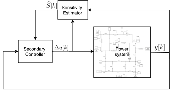
In this section, we present the secondary controller that relies on the output prediction model for regulating the system output to the nominal value, and the learned power-voltage characteristics of the PV arrays for dealing with uncertainty in solar power generation. Figure 1 depicts the diagram of the proposed controller. The sensitivity estimator in (9) is executed in parallel with the controller. Specifically, the applied control input adjustment and the measured resulting change in the output, , are provided to the estimator to further update the sensitivity matrix estimate, , using (9). Controller performance depends on the accuracy of the prediction model decided by the richness of the control input adjustments. This motivates the strategy used in this paper to allow the proposed controller to generate persistently exciting control inputs.
IV-A Feedback Optimization with Persistent Excitation
In the following, we present the secondary controller as a solver of some underlying optimization problem. We begin with the following optimization problem:
| (16a) | ||||
| subject to | (16b) | |||
where , , , , with and denoting respectively the lower and upper bounds on the active power setpoint adjustment at inverter at time instant , and and denoting the lower and upper bounds on the reactive power setpoint adjustment at inverter at time instant . The objective is to produce the output change that tracks the target while penalizing the control effort. The inequality constraints (16b) are meant for keeping the input adjustments within the incremental capacities of the inverters and inside the linear regime where the linear prediction model is accurate. We then excite the control input adjustments by adding a random signal, denoted by , to the solution of the optimization problem (16), denoted by , as follows:
| (17) |
Despite the simplicity of the excitation approach, there exist several challenges in choosing suitable values for . On the one hand, needs to be large enough in order for its effect to be measurable at the output. On the other hand, if is too large, the control input adjustments might push the operating point away from the desired one degrading the controller performance. Even more importantly, (17) does not take into account random variations in , e.g., due to load fluctuations, which can add a significant amount of excitation to , making the excitation via the addition of unnecessary. In what follows, we describe an alternative approach for exciting the secondary control commands, where we make use of the random variations in as appropriate, and avoid unnecessary excitation that (17) might generate.
Consider the following modification of the optimization problem (16), where we add a random signal, denoted by , to the target :
| subject to |
where , if is persistently exciting, and , with , otherwise, where denotes the continuous uniform distribution over the interval . For the time being, we neglect the inequality constraints in the following discussion. It holds trivially that if is invertible for all , then, adding to the target will generate persistently exciting sequence . However, if has more columns than rows, then, adding will provide excitation in the subspace that is orthogonal to the null space of . This opens up the possibility of the sequence not being persistently exciting. To rule out such possibility, we excite the control input adjustments as follows:
| (18) |
if is persistently exciting, and
| (19) |
otherwise, where and are randomly chosen such that 22 2 denotes the null space of an matrix , i.e., and
| (20) |
Since , we note that the perturbation does not affect the predicted output change, . Hence, if the prediction model is accurate, we expect the perturbation not to have any effect on the system output.
Next, we discuss the control excitation taking into account the inequality constraints. The inequality constraints might become active if the target is sufficiently large. As a result, the control input adjustments may not be excitable without violating the inequality constraints, namely, there might not exist non-zero such that (20) holds. To guard against such possibility, we keep the control input adjustments persistently exciting by randomly varying the lower and upper bounds of the constraints in (16b), yielding the following optimization problem:
| (21a) | ||||
| subject to | (21b) | |||
where , , with , at time instant . Note that if all inequality constraints are active at the solution, then, the approach is equivalent to (17). On the other hand, if only a subset of the inequality constraints are active, then, the target plays a non-negligible role in exciting the solution . The pseudocode for the proposed secondary control approach is provided in Algorithm 1.
Algorithm 1. Data-Driven Secondary Control with Persistent Excitation.
1. Initialize , , .
2. Set , if is persistently exciting, and , otherwise; ; .
3. Find a solution of (21), , and
apply
if is persistently exciting,
and
otherwise, where and are randomly chosen such that and
IV-B Secondary Control with PV Power Tracking
In the following, we take into consideration the constraints that PV arrays impose on the secondary controller during its execution. As discussed earlier, to extract a desired amount of power from a PV array, a certain voltage must be applied across its terminals, as determined by its power-voltage characteristic. Hence, the voltage setpoint must be computed so as to allow the PV array to track the secondary control inputs. To this end, we augment the optimization problem (21) with the learned power-voltage characteristics (2) as follows:
| (22a) | ||||
| subject to | (22b) | |||
| (22c) | ||||
| (22d) | ||||
| (22e) | ||||
where , represents the estimated power-voltage characteristic of the PV array , with denoting the estimated coefficients of the fitted polynomial model, and denote the lower and upper bounds on the voltage applied across the terminals of the PV array , and , with denoting the active power injection by the PV array at time . The constraint (22d) serves to maintain a power balance between the generated solar power and the inverter active power output, while neglecting the inverter losses. Note that we have integrated step 4 of Algorithm 1 directly into the optimization (22), where , if is persistently exciting, and is randomly chosen, otherwise. Due to the non-linearity of the power-voltage characteristics in (22d), the problem (22) is non-convex. However, as described next, it has an equivalent convex reformulation comprising two stages.
In the first stage, we consider the following convex relaxation of (22), where the power-voltage characteristics are replaced with the inequality constraints that are meant to keep the control input adjustments within the incremental capacities of the PV arrays:
| (23a) | ||||
| subject to | (23b) | |||
| (23c) | ||||
| (23d) | ||||
where , and denote the maximum and minimum incremental capacities of the PV array , and denotes the estimate of the active power capacity of the PV array . In (23), we are content with finding the power setpoints that are to be tracked by the PV arrays given their limited incremental capacities. To find the corresponding voltage setpoints, we execute the second stage as follows. We compute the voltage setpoint of the PV array , denoted by , such that , with denoting the solution of (23), by using the power tracking algorithm in [13, Algorithm 2], which is based on Newton’s method.
Since it is easy to see that is the solution of (22), we omit the proof. Inclusion of the inequality constraints in (23d) may lead to a lack of persistent excitation of the control inputs. Similar to (21), to guard against such possibility, we randomly vary the lower and upper bounds of the constraints in (23d) if the incremental capacities of the PV arrays are not persistently exciting, yielding the following optimization problem:
| (24a) | ||||
| subject to | (24b) | |||
| (24c) | ||||
| (24d) | ||||
where , if is persistently exciting, and , otherwise, with , at time instant ; , if is persistently exciting, and , otherwise. In Algorithm 2, we provide the pseudocode for the proposed approach combining the secondary control objectives with the PV power tracking objectives.
Algorithm 2. Data-Driven Secondary Control with PV Power Tracking. 1. Initialize , , , . 2. Set , if is persistently exciting, and , otherwise; ; ; , if is persistently exciting, and , otherwise; , if is persistently exciting, and , otherwise; , if is persistently exciting, and is randomly chosen, otherwise; is randomly chosen such that . 3. Find a solution of (24), , and apply . 4. Compute such that , , by using [13, Algorithm 2].
V Numerical Simulations
We showcase the proposed secondary controller using a modified version of the IEEE-14 bus test system [15], with energy sources providing both active and reactive power at buses , , , and reactive power energy sources at buses and replaced by inverter-interfaced DERs, as described in the single line diagram of the test system in Figure 2. The GFM-inverter-interfaced DERs are located at buses , and , and the GFL inverters interfacing PV arrays are located at buses and . The DER index sets are given by: , and .
PV generation is simulated at buses and using solar irradiance data collected from NREL’s Oahu Solar Measurement Grid [16] on Oct 1, 2011, from 11:56:40 am to 12:00:00 pm; see Figure 3. As described in Section II-C, the estimation of the power-voltage characteristics of the PV arrays at buses and is performed by fitting the polynomial models in (2), with , to the collected power-voltage measurements and , with . Figure 3 also shows the maximum available solar power at bus and its estimate obtained from the learned power-voltage characteristics.
Load perturbations occur every s, and the secondary controller is executed every s except for the time instants when the loads are perturbed. This separation between the controller actions and load changes is introduced to clearly demonstrate the effectiveness of the control approach. Otherwise, if the loads change while the system is settling down after a secondary controller execution, it is more challenging to evaluate the controller performance and the accuracy of the prediction model.
We execute Algorithm 1 to determine the control input adjustments, and use the following values to initialize its parameters: , , , pu, pu, , and . The feedback optimization problem (23) is solved using CVXPY [17]. The sensitivity estimator in (9) is executed in parallel with the controller. Specifically, the applied control input adjustment and the measured resulting change in the output, , are provided to the estimator to further update the sensitivity matrix estimate, , using (9). The estimator is initialized using (15). We also use the following values to initialize the estimator parameters in (9): , .
Figure 4 shows the evolution of the system output, namely, the system frequency and voltage magnitudes at buses , , being regulated to the corresponding nominal values, Hz, pu, pu, and pu, and the active power flow through line kept below its thermal limit set at pu. To be more specific, this figure shows the steady-state values of the system output after each load perturbation, and after each secondary control action. [Note that three control actions are taken before another load perturbation occurs.] It can be seen that the control actions determined by Algorithm 1 manage to keep the system output close to the nominal values despite the system experiencing significant load variations. We note that the control actions do not always bring the system output noticeably closer to their nominal values, because the controller constantly makes a tradeoff between various objectives—frequency regulation, line flow regulation, and voltage regulation—while satisfying the constraints on the control input adjustments.
Figure 5 shows the evolution of the estimates of the sensitivities corresponding to the system frequency. During the first s, the sensitivity estimates experience some transients quickly reaching a steady state. Note that the initial estimates are not far away from the steady-state ones, which explains the satisfactory performance of the controller in regulating frequency during the transient period. Also note that the active power setpoint adjustments, , have much more significant effect on the frequency than the reactive power setpoint adjustments, , which is consistent with the inductive nature of the test system network. The smallest and largest eigenvalues of , with , are bounded and strictly positive and equal, on average, and , demonstrating that satisfies (7), and, thus, is persistently exciting.
Figure 5 also shows the predictions of the system frequency made by the linear prediction model based on the learned sensitivities. Prediction errors are less than % in % of all test cases, where the prediction errors are computed as follows:
where is the prediction error corresponding to the output change , is the threshold below which the changes in the output are not measurable. For example, for the system frequency, we set Hz. We note that the predictions are less accurate during the initial transient period, when the operating point changes significantly, or when the control input adjustments are too large going over the linear regime of the prediction model.
VI Concluding Remarks and Future Work
In this paper, we developed a data-driven secondary controller for power networks with a deep penetration of GFM inverters. The controller, which is based on feedback optimization, relies on learning specific power system sensitivities, e.g., of the system frequency to the inverter setpoints, for predicting the system output changes given the input adjustments. It is critical to keep the feedback optimization solution persistently exciting in order to be able to make accurate predictions. To this end, we presented an approach that maintains persistent excitation of the control inputs without significantly degrading the controller performance.
One of the future directions that we intend to explore is to utilize a more sophisticated prediction model in the feedback optimization to improve prediction accuracy. However, in the case of standard polynomial models or linear transfer function models (see, e.g., [12]), predictions were less accurate in our simulations.
References
- [1] K. Zhou, C. Fu, and S. Yang, “Big data driven smart energy management: From big data to big insights,” Renewable and Sustainable Energy Reviews, vol. 56, pp. 215–225, 2016.
- [2] C. De Persis and P. Tesi, “Formulas for data-driven control: Stabilization, optimality, and robustness,” IEEE Transactions on Automatic Control, vol. 65, no. 3, pp. 909–924, 2020.
- [3] Y. C. Chen, A. D. Domínguez-García, and P. W. Sauer, “Measurement-based estimation of linear sensitivity distribution factors and applications,” IEEE Transactions on Power Systems, vol. 29, no. 3, pp. 1372–1382, 2014.
- [4] K. E. Van Horn, A. D. Domínguez-García, and P. W. Sauer, “Measurement-based real-time security-constrained economic dispatch,” IEEE Transactions on Power Systems, vol. 31, no. 5, pp. 3548–3560, 2016.
- [5] P. Hidalgo-Gonzalez, R. Henriquez-Auba, D. S. Callaway, and C. J. Tomlin, “Frequency regulation using data-driven controllers in power grids with variable inertia due to renewable energy,” in Proc. IEEE Power Energy Society General Meeting, 2019, pp. 1–5.
- [6] H. Xu, A. D. Domínguez-García, and P. W. Sauer, “Data-driven coordination of distributed energy resources for active power provision,” IEEE Transactions on Power Systems, vol. 34, no. 4, pp. 3047–3058, 2019.
- [7] S. Karagiannopoulos, R. Dobbe, P. Aristidou, D. Callaway, and G. Hug, “Data-driven control design schemes in active distribution grids: Capabilities and challenges,” in Proc. IEEE PowerTech, 2019, pp. 1–6.
- [8] H. Xu, A. D. Domínguez-García, V. V. Veeravalli, and P. W. Sauer, “Data-driven voltage regulation in radial power distribution systems,” IEEE Transactions on Power Systems, vol. 35, no. 3, pp. 2133–2143, 2020.
- [9] S. S. Madani, C. Kammer, and A. Karimi, “Data-driven distributed combined primary and secondary control in microgrids,” IEEE Transactions on Control Systems Technology, pp. 1–8, 2020.
- [10] Y. Chen, Y. Shi, and B. Zhang, “Data-driven optimal voltage regulation using input convex neural networks,” Electric Power Systems Research, vol. 189, p. 106741, 2020.
- [11] Q. Yang, G. Wang, A. Sadeghi, G. B. Giannakis, and J. Sun, “Two-timescale voltage control in distribution grids using deep reinforcement learning,” IEEE Transactions on Smart Grid, vol. 11, no. 3, pp. 2313–2323, 2020.
- [12] K. J. Åström and B. Wittenmark, Adaptive Control: Second Edition. Mineola, New York: Dover, 2008.
- [13] X. Zhang, V. Purba, M. Hong, and S. Dhople, “A sum-of-squares optimization method for learning and controlling photovoltaic systems,” in Proc. American Control Conference, 2020, pp. 2376–2381.
- [14] M. Lu, S. Dutta, V. Purba, S. Dhople, and B. Johnson, “A grid-compatible virtual oscillator controller: Analysis and design,” in Proc. IEEE Energy Conversion Congress and Exposition, 2019, pp. 2643–2649.
- [15] IEEE 14-Bus System, Power Systems Test Case Archive, https://www.ece.uw.edu/research/pstca/pf14/pg_tca14bus.htm.
- [16] M. Sengupta and A. Andreas, “Oahu Solar Measurement Grid (1-Year Archive): 1-Second Solar Irradiance; Oahu, Hawaii (Data),” NREL Report No. DA-5500-56506, 2010.
- [17] S. Diamond and S. Boyd, “CVXPY: A Python-embedded modeling language for convex optimization,” Journal of Machine Learning Research, vol. 17, no. 83, pp. 1–5, 2016.