跳到论文正文
W Papers独立论文阅读器 arXiv:2102.01752 论文正文 计算阅读时间 · 0%
引用这篇论文根据当前论文元数据生成,正式投稿前建议核对。


License: arXiv.org perpetual non-exclusive license
arXiv:2102.01752v1 [cs.LG] 02 Feb 2021

Continuous Wasserstein-2 Barycenter
Estimation without Minimax Optimization

Alexander Korotin Affiliation: Skolkovo Institute of Science and Technology Affiliation: Advanced Data Analytics in Science and Affiliation: Engineering Group Affiliation: Moscow, Russia Email: a.korotin@skoltech.ru    Lingxiao Li Affiliation: Massachusetts Institute of Technology Affiliation: Geometric Data Processing Group Affiliation: Cambridge, Massachusetts, USA Email: lingxiao@mit.edu    Justin Solomon Affiliation: Massachusetts Institute of Technology Affiliation: Geometric Data Processing Group Affiliation: Cambridge, Massachusetts, USA Email: jsolomon@mit.edu    Evgeny Burnaev Affiliation: Skolkovo Institute of Science and Technology Affiliation: Advanced Data Analytics in Science Affiliation: and Engineering Group Affiliation: Moscow, Russia Email: e.burnaev@skoltech.ru
Abstract

Wasserstein barycenters provide a geometric notion of the weighted average of probability measures based on optimal transport. In this paper, we present a scalable algorithm to compute Wasserstein-2 barycenters given sample access to the input measures, which are not restricted to being discrete. While past approaches rely on entropic or quadratic regularization, we employ input convex neural networks and cycle-consistency regularization to avoid introducing bias. As a result, our approach does not resort to minimax optimization. We provide theoretical analysis on error bounds as well as empirical evidence of the effectiveness of the proposed approach in low-dimensional qualitative scenarios and high-dimensional quantitative experiments.

1 Introduction

Wasserstein barycenters have become popular due to their ability to represent the average of probability measures in a geometrically meaningful way. Techniques for computing Wasserstein barycenters have been successfully applied to many computational problems. In image processing, Wasserstein barycenters are used for color and style transfer (Rabin et al. 2014; Mroueh 2019), and texture synthesis (Rabin et al. 2011). In geometry processing, shape interpolation can be done by computing barycenters (Solomon et al. 2015). In online machine learning, barycenters are used for aggregating probabilistic predictions of experts (Korotin et al. 2019b). Within the context of Bayesian inference, the barycenter of subset posteriors converges to the full data posterior, thus enabling efficient computational methods based on finding the barycenters (Srivastava et al. 2015; Srivastava et al. 2018).

Fast and accurate barycenter algorithms exist for discrete distributions (see Peyré et al. 2019 for a survey), while for continuous distributions the situation is more difficult and remains unexplored until recently (Li et al. 2020; Fan et al. 2020; Cohen et al. 2020). The discrete methods scale poorly with the number of support points of the barycenter and thus cannot approximate continuous barycenters well, especially in high dimensions.

In this paper, we present a method to compute Wasserstein-2 barycenters of continuous distributions based on a novel regularized dual formulation where the convex potentials are parameterized by input convex neural networks (Amos et al. 2017). Our algorithm is straightforward without introducing bias (e.g. Li et al. 2020) or requiring minimax optimization (e.g. Fan et al. 2020). This is made possible by combining a new congruence regularizing term combined with cycle-consistency regularization (Korotin et al. 2019a). As we will show in the analysis, thanks to the properties of Wasserstein-2 distances, the gradients of the resulting convex potentials “push” the input distributions close to the true barycenter, allowing good approximation of the barycenter.

2 Preliminaries

We denote the set of all Borel probability measures on ℝD\mathbb{R}^{D} with finite second moment by 𝒫2​(ℝD)\mathcal{P}_{2}(\mathbb{R}^{D}). We use 𝒫2,ac​(ℝD)⊂𝒫2​(ℝD)\mathcal{P}_{2,\text{ac}}(\mathbb{R}^{D})\subset\mathcal{P}_{2}(\mathbb{R}^{D}) to denote the subset of all absolutely continuous measures (w.r.t. the Lebesgue measure).

Wasserstein-2 distance.

For ℙ,ℚ∈𝒫2​(ℝD)\mathbb{P},\mathbb{Q}\in\mathcal{P}_{2}(\mathbb{R}^{D}), the Wasserstein-2 distance is defined by

𝕎22​(ℙ,ℚ)=defmin⁡∫ℝD×ℝDπ∈Π⁡(ℙ,ℚ)⁡‖x−y‖22​𝑑π​(x,y),\mathbb{W}_{2}^{2}(\mathbb{P},\mathbb{Q})\stackrel{{\scriptstyle\text{def}}}{{=}}\min_{\pi\in\Pi(\mathbb{P},\mathbb{Q})}\int_{\mathbb{R}^{D}\times\mathbb{R}^{D}}\frac{\|x-y\|^{2}}{2}d\pi(x,y), (1)

where Π⁡(ℙ,ℚ)\Pi(\mathbb{P},\mathbb{Q}) is the set of probability measures on ℝD×ℝD\mathbb{R}^{D}\times\mathbb{R}^{D} whose marginals are ℙ,ℚ\mathbb{P},\mathbb{Q}, respectively. This definition is known as Kantorovich’s primal form of transport distance (Kantorovitch 1958).

The Wasserstein-2 distance 𝕎2\mathbb{W}_{2} is well-studied in the theory of optimal transport (Brenier 1991; McCann et al. 1995). In particular, it has a dual formulation (Villani 2003):

𝕎22​(ℙ,ℚ)=∫ℝD‖x‖22​𝑑ℙ​(x)+∫ℝD‖y‖22​𝑑ℚ​(y)−minψ∈Conv⁡[∫ℝDψ⁡(x)​𝑑ℙ​(x)+∫ℝDψ¯​(y)​𝑑ℚ​(y)],\displaystyle\mathbb{W}_{2}^{2}(\mathbb{P},\mathbb{Q})=\int_{\mathbb{R}^{D}}\frac{\|x\|^{2}}{2}d\mathbb{P}(x)+\int_{\mathbb{R}^{D}}\frac{\|y\|^{2}}{2}d\mathbb{Q}(y)-\min_{\psi\in\text{Conv}}\bigg[\int_{\mathbb{R}^{D}}\psi(x)d\mathbb{P}(x)+\int_{\mathbb{R}^{D}}\overline{\psi}(y)d\mathbb{Q}(y)\bigg], (2)

where the minimum is taken over all the convex functions (potentials) ψ:ℝD→ℝ∪{∞}\psi:\mathbb{R}^{D}\rightarrow\mathbb{R}\cup\{\infty\}, and ψ¯​(y)=maxx∈ℝD⁡(⟨x,y⟩−ψ⁡(x)):ℝD→ℝ∪{∞}\overline{\psi}(y)=\max_{x\in\mathbb{R}^{D}}\big(\langle x,y\rangle-\psi(x)\big):\mathbb{R}^{D}\rightarrow\mathbb{R}\cup\{\infty\} is the convex conjugate of ψ\psi (Fenchel 1949), which is also a convex function. The optimal potential ψ∗\psi^{*} is defined up to an additive constant.

Brenier 1991 shows that if ℙ\mathbb{P} does not give mass to sets of dimensions at most D−1D-1, then the optimal plan π\pi is uniquely determined by π∗=[idℝD,T∗]​♯​ℙ\pi^{*}=[\text{id}_{\mathbb{R}^{D}},T^{*}]\sharp\mathbb{P}, where T∗:ℝD→ℝDT^{*}:\mathbb{R}^{D}\rightarrow\mathbb{R}^{D} is the unique solution to the Monge’s problem

T∗=arg​minT​♯​ℙ=ℚ∫ℝD‖x−T⁡(x)‖22dℙ(x).T^{*}=\argmin_{T\sharp\mathbb{P}=\mathbb{Q}}\int_{\mathbb{R}^{D}}\frac{\|x-T(x)\|^{2}}{2}d\mathbb{P}(x). (3)

The connection between T∗T^{*} and the dual formulation (2) is that T∗=∇ψ∗T^{*}=\nabla\psi^{*}, where ψ∗\psi^{*} is the optimal solution of (2). Additionally, if ℚ\mathbb{Q} does not give mass to sets of dimensions at most D−1D-1, then T∗T^{*} is invertible and

T∗​(x)=∇ψ∗​(x)=(∇ψ∗¯)−1​(x),(T∗)−1​(y)=∇ψ∗¯​(y)=(∇ψ∗)−1​(y).T^{*}(x)=\nabla\psi^{*}(x)=(\nabla\overline{\psi^{*}})^{-1}(x),\qquad(T^{*})^{-1}(y)=\nabla\overline{\psi^{*}}(y)=(\nabla\psi^{*})^{-1}(y).

In particular, the above discussion applies to the case where ℙ,ℚ∈𝒫2,a​c​(ℝD)\mathbb{P},\mathbb{Q}\in\mathcal{P}_{2,ac}(\mathbb{R}^{D}).

Wasserstein-2 barycenter.

Let ℙ1,…,ℙN∈𝒫2,a​c​(ℝD)\mathbb{P}_{1},\dots,\mathbb{P}_{N}\in\mathcal{P}_{2,ac}(\mathbb{R}^{D}). Then, their barycenter w.r.t. weights α1,…,αN\alpha_{1},\dots,\alpha_{N} (αn>0\alpha_{n}>0 and ∑n=1Nαn=1\sum_{n=1}^{N}\alpha_{n}=1) is

ℙ¯=defarg​minℙ∈𝒫2​(ℝD)∑n=1Nαn𝕎22(ℙn,ℙ).\overline{\mathbb{P}}\stackrel{{\scriptstyle\text{def}}}{{=}}\argmin_{\mathbb{P}\in\mathcal{P}_{2}(\mathbb{R}^{D})}\sum_{n=1}^{N}\alpha_{n}\mathbb{W}_{2}^{2}(\mathbb{P}_{n},\mathbb{P}). (4)

Throughout this paper, we assume that at least one of ℙ1,…,ℙN∈𝒫2,a​c​(ℝD){\mathbb{P}_{1},\dots,\mathbb{P}_{N}\in\mathcal{P}_{2,ac}(\mathbb{R}^{D})} has bounded density. Under this assumption, ℙ¯\overline{\mathbb{P}} is unique and absolutely continuous, i.e., ℙ¯∈𝒫2,a​c​(ℝD)\overline{\mathbb{P}}\in\mathcal{P}_{2,ac}(\mathbb{R}^{D}), and it has bounded density (Agueh & Carlier 2011, Definition 3.6 & Theorem 5.1).

For n∈{1,2,…,N}n\in\{1,2,\dots,N\}, let (ψn∗,ψn∗¯)(\psi^{*}_{n},\overline{\psi^{*}_{n}}) be the optimal pair of (mutually) conjugate potentials that transport ℙn\mathbb{P}_{n} to ℙ¯\overline{\mathbb{P}}, i.e., ∇ψ∗n♯ℙn=ℙ¯\nabla\psi^{*}_{n}\sharp\mathbb{P}_{n}=\overline{\mathbb{P}} and ∇ψn∗¯♯ℙ¯=ℙn\nabla\overline{\psi^{*}_{n}}\sharp\overline{\mathbb{P}}=\mathbb{P}_{n}. Then {ψn∗¯}\{\overline{\psi^{*}_{n}}\} satisfy

∑n=1Nαn∇ψn∗¯(x)=xand∑n=1Nαnψn∗¯(x)=‖x‖22+c.\sum_{n=1}^{N}\alpha_{n}\nabla\overline{\psi^{*}_{n}}(x)=x\qquad\text{and}\qquad\sum_{n=1}^{N}\alpha_{n}\overline{\psi^{*}_{n}}(x)=\frac{\|x\|^{2}}{2}+c. (5)

for all x∈ℝDx\in\mathbb{R}^{D} (Agueh & Carlier 2011; Álvarez-Esteban et al. 2016). Since optimal potentials are defined up to a constant, for convenience, we set c=0c=0. The condition (5) serves as the basis for our algorithm for computing Wasserstein-2 barycenters. We say that potentials ψ1,…,ψN\psi_{1},\dots,\psi_{N} are congruent w.r.t. weights α1,…,αn\alpha_{1},\dots,\alpha_{n} if their conjugate potentials satisfy (5), i.e., ∑n=1Dαn​ψn¯​(x)=‖x‖22\sum_{n=1}^{D}\alpha_{n}\overline{\psi_{n}}(x)=\frac{\|x\|^{2}}{2} for all x∈ℝDx\in\mathbb{R}^{D}.

3 Related Work

Most algorithms in the field of computational optimal transport are designed for the discrete setting where the input distributions have finite support; see the recent survey by Peyré et al. 2019 for discussion. A particular popular line of algorithms are based on entropic regularization that gives rise to the famous Sinkhorn iteration (Cuturi 2013; Cuturi & Doucet 2014). These methods are typically limited to a support of 105−10610^{5}\!-\!10^{6} points before the problem becomes computationally infeasible. Similarly, discrete barycenter methods (Cuturi & Doucet 2014), particularly the ones that rely on a fixed support for the barycenter (Dvurechenskii et al. 2018; Staib et al. 2017), cannot provide precise approximation of continuous barycenters in high dimensions, since a large number of samples is needed; see experiments in Fan et al. 2020 for an example. Thus we focus on the existing literature in the continuous setting.

Computation of Wasserstein-2 distances and maps.

Genevay et al. 2016 demonstrate the possibility of computing Wasserstein distances given only sample access to the distributions by parameterizing the dual potentials as functions in the reproducing kernel Hilbert spaces. Based on this realization, Seguy et al. 2017 propose a similar method but use neural networks to parameterize the potentials, using entropic or ℒ2\mathcal{L}^{2} regularization w.r.t. ℙ×ℚ\mathbb{P}\times\mathbb{Q} to keep the potentials approximately conjugate. The transport map is recovered from optimized potentials via barycentric projection.

As we note in §2, 𝕎2\mathbb{W}_{2} enjoys many useful theoretical properties. For example, the optimal potential ψ∗\psi^{*} is convex, and the corresponding optimal transport map is given by ∇ψ∗\nabla\psi^{*}. By exploiting these properties, Makkuva et al. 2019 propose a minimax optimization algorithm for recovering transport maps, using input convex neural networks (ICNNs) (Amos et al. 2017) to approximate the potentials.

An alternative to entropic regularization is the cycle-consistency regularization proposed by Korotin et al. 2019a. It uses the property that the gradients of optimal dual potentials are inverses of each other. The imposed regularizer requires integration only over the marginal measures ℙ\mathbb{P} and ℚ\mathbb{Q}, instead of over ℙ×ℚ\mathbb{P}\times\mathbb{Q} as required by entropy-based alternatives. Their method converges faster than the minimax method since it does not have an inner optimization cycle.

Xie et al. 2019 propose using two generative models with a shared latent space to implicitly compute the optimal transport correspondence between ℙ\mathbb{P} and ℚ\mathbb{Q}. Based on the obtained correspondence, the authors are able to compute the optimal transport distance between the distributions.

Computation of Wasserstein-2 barycenters.

A few recent techniques tackle the barycenter problem (4) using continuous rather than discrete approximations of the barycenter:

  • •

    Measure-based (generative) optimization: Problem (4) optimizes over probability measures. This can be done using the generic algorithm by Cohen et al. 2020 who employ generative networks to compute barycenters w.r.t. arbitrary discrepancies. They test their method with the maximum mean discrepancy (MMD) and Sinkhorn divergence. This approach suffers from the usual limitations of generative models such as mode collapse. Applying it to 𝕎2\mathbb{W}_{2} barycenters requires estimation of 𝕎22​(ℙn,ℙ)\mathbb{W}_{2}^{2}(\mathbb{P}_{n},\mathbb{P}). Fan et al. 2020 test this approach using the minimax method by Makkuva et al. 2019, but they end up with a challenging min-max-min problem.

  • •

    Potential-based optimization: Li et al. 2020 recover the optimal potentials {ψn∗}\{\psi^{*}_{n}\} via a non-minimax regularized dual formulation. No generative model is needed: the barycenter is recovered by pushing forward measures using gradients of potentials or by barycentric projection.

4 Methods

Inspired by Li et al. 2020 we use a potential-based approach and recover the barycenter by using gradients of the potentials as pushforward maps. The main differences are: (1) we restrict the potentials to be convex, (2) we enforce congruence via a regularizing term, and (3) our formulation does not introduce bias, meaning the optimal solution of our formulation gives the true barycenter.

4.1 Deriving the Dual Problem

Let ℙ¯\overline{\mathbb{P}} be the true barycenter. Our goal is to recover the optimal potentials {ψn∗,ψn∗¯}\{\psi_{n}^{*},\overline{\psi_{n}^{*}}\} mapping the input measures ℙn\mathbb{P}_{n} into ℙ¯\overline{\mathbb{P}}.

To start, we express the barycenter objective (4) after substituting the dual formulation (2):

∑n=1Nαn​𝕎22​(ℙn,ℙ¯)=[∑n=1Nαn​∫ℝD‖x‖22​d​ℙn​(x)]+∫ℝD‖y‖22​𝑑ℙ¯​(y)−\displaystyle\sum_{n=1}^{N}\alpha_{n}\mathbb{W}_{2}^{2}(\mathbb{P}_{n},\overline{\mathbb{P}})=\bigg[\sum_{n=1}^{N}\alpha_{n}\int_{\mathbb{R}^{D}}\frac{\|x\|^{2}}{2}d\mathbb{P}_{n}(x)\bigg]+\int_{\mathbb{R}^{D}}\frac{\|y\|^{2}}{2}d\overline{\mathbb{P}}(y)-
min{ψn}∈Conv⁡[∑n=1Nαn​∫ℝDψn​(x)​d​ℙn​(x)+∑n=1Nαn​∫ℝDψn¯​(y)​𝑑ℙ¯​(y)]\displaystyle\min_{\{\psi_{n}\}\in\text{Conv}}\bigg[\sum_{n=1}^{N}\alpha_{n}\int_{\mathbb{R}^{D}}\psi_{n}(x)d\mathbb{P}_{n}(x)+\sum_{n=1}^{N}\alpha_{n}\int_{\mathbb{R}^{D}}\overline{\psi_{n}}(y)d\overline{\mathbb{P}}(y)\bigg] (6)

The minimum is attained not just among convex potentials {ψn}\{\psi_{n}\}, but among congruent potentials (see discussion under (5)); thus, we can add the constraint that {ψn}\{\psi_{n}\} are congruent to (6). Hence,

∑n=1Nαn​𝕎22​(ℙn,ℙ¯)=[∑n=1Nαn​∫ℝD‖x‖22​d​ℙn​(x)]−min{ψn}​ congruent⁡[∑n=1Nαn​∫ℝDψn​(y)​d​ℙn​(y)⏟MultiCorr​({αn,ℙn}|{ψn})].\displaystyle\sum_{n=1}^{N}\alpha_{n}\mathbb{W}_{2}^{2}(\mathbb{P}_{n},\overline{\mathbb{P}})=\bigg[\sum_{n=1}^{N}\alpha_{n}\int_{\mathbb{R}^{D}}\frac{\|x\|^{2}}{2}d\mathbb{P}_{n}(x)\bigg]-\!\!\!\min_{\{\psi_{n}\}\text{ congruent}}\bigg[\underbrace{\sum_{n=1}^{N}\alpha_{n}\int_{\mathbb{R}^{D}}\!\!\psi_{n}(y)d\mathbb{P}_{n}(y)}_{\text{MultiCorr}(\{\alpha_{n},\mathbb{P}_{n}\}|\{\psi_{n}\})}\bigg]. (7)

To transition from (6) to (7), we used the fact that for congruent {ψn}\{\psi_{n}\} we have ∑n=1Nαn​ψn¯​(x)=‖x‖22{\sum_{n=1}^{N}\alpha_{n}\overline{\psi_{n}}(x)=\frac{\|x\|^{2}}{2}}, so ∑n=1N∫ℝDαn​ψn¯​(y)​𝑑ℙ¯​(y)=∫ℝD‖y‖22​𝑑ℙ¯​(y).\sum_{n=1}^{N}\int_{\mathbb{R}^{D}}\alpha_{n}\overline{\psi_{n}}(y)d\overline{\mathbb{P}}(y)=\int_{\mathbb{R}^{D}}\frac{\|y\|^{2}}{2}d\overline{\mathbb{P}}(y).

We call the value inside the minimum in (7) the multiple correlation of {ℙn}\{\mathbb{P}_{n}\} with weights {αn}\{\alpha_{n}\} w.r.t. potentials {ψn}\{\psi_{n}\}. Notice that the true barycenter ℙ¯\overline{\mathbb{P}} appears nowhere on the right side of (7). Thus the optimal potentials {ψn∗}\{\psi_{n}^{*}\} can be recovered by solving the following

min{ψn}​ congruent⁡MultiCorr​({αn,ℙn}|{ψn})=min{ψn}​ congruent⁡[∑n=1Nαn​∫ℝDψn​(y)​d​ℙn​(y)].\displaystyle\min_{\{\psi_{n}\}\text{ congruent}}\text{MultiCorr}(\{\alpha_{n},\mathbb{P}_{n}\}|\{\psi_{n}\})=\min_{\{\psi_{n}\}\text{ congruent}}\bigg[\sum_{n=1}^{N}\alpha_{n}\int_{\mathbb{R}^{D}}\!\!\psi_{n}(y)d\mathbb{P}_{n}(y)\bigg]. (8)

4.2 Imposing the Congruence Condition

It is challenging to impose the congruence condition on convex potentials. What if we relax the congruence condition? The following theorem bounds how close a set of convex potentials {ψn}\{\psi_{n}\} is to {ψn∗}\{\psi_{n}^{*}\} in terms of the difference of multiple correlation.

Theorem 4.1.

Let ℙ¯∈𝒫2,a​c​(ℝD)\overline{\mathbb{P}}\in\mathcal{P}_{2,ac}(\mathbb{R}^{D}) be the barycenter of ℙ1,…,ℙN∈𝒫2,a​c​(ℝD)\mathbb{P}_{1},\dots,\mathbb{P}_{N}\in\mathcal{P}_{2,ac}(\mathbb{R}^{D}) w.r.t. weights α1,…,αN\alpha_{1},\dots,\alpha_{N}. Let {ψn∗}\{\psi_{n}^{*}\} be the optimal congruent potentials of the barycenter problem. Suppose we have ℬ\mathcal{B}-smooth11 1 We say that a diffirentiable function f:ℝD→ℝf:\mathbb{R}^{D}\rightarrow\mathbb{R} is ℬ\mathcal{B}-smooth if its gradient ∇f\nabla f is ℬ\mathcal{B}-Lipschitz. convex potentials {ψn}\{\psi_{n}\} for some ℬ∈[0,+∞]\mathcal{B}\in[0,+\infty], and denote Δ=MultiCorr​({αn,ℙn}∣{ψn})−MultiCorr​({αn,ℙn}∣{ψn∗})\Delta=\text{MultiCorr}(\{\alpha_{n},\mathbb{P}_{n}\}\mid\{\psi_{n}\})-\text{MultiCorr}(\{\alpha_{n},\mathbb{P}_{n}\}\mid\{\psi^{*}_{n}\}). Then,

Δ+∫ℝD∑n=1N[αn​ψn¯​(y)−‖y‖22]​dℙ¯​(y)⏟Congruence mismatch≥12​ℬ​∑n=1Nαn​‖∇ψn∗​(x)−∇ψn​(x)‖ℙn2.\displaystyle\Delta+\underbrace{\int_{\mathbb{R}^{D}}\sum_{n=1}^{N}\big[\alpha_{n}\overline{\psi_{n}}(y)-\frac{\|y\|^{2}}{2}\big]d\overline{\mathbb{P}}(y)}_{\text{Congruence mismatch}}\geq\frac{1}{2\mathcal{B}}\sum_{n=1}^{N}\alpha_{n}\|\nabla\psi_{n}^{*}(x)-\nabla\psi_{n}(x)\|^{2}_{\mathbb{P}_{n}}. (9)

Here ∥⋅∥μ\|\cdot\|_{\mu} denotes the norm induced by inner product in Hilbert space ℒ2(ℝD→ℝD,μ)\mathcal{L}^{2}(\mathbb{R}^{D}\rightarrow\mathbb{R}^{D},\mu). We call the second term on the left of (9) the congruence mismatch.

We prove this in Appendix B. Note that if the congruence mismatch is non-positive, then

Δ≥12​ℬ∑n=1Nαn∥∇ψn∗(x)−∇ψn(x)∥ℙn2≥1ℬ∑n=1Nαn𝕎22(∇ψn♯ℙn,ℙ¯),\Delta\geq\frac{1}{2\mathcal{B}}\sum_{n=1}^{N}\alpha_{n}\|\nabla\psi_{n}^{*}(x)-\nabla\psi_{n}(x)\|^{2}_{\mathbb{P}_{n}}\geq\frac{1}{\mathcal{B}}\sum_{n=1}^{N}\alpha_{n}\mathbb{W}_{2}^{2}(\nabla\psi_{n}\sharp\mathbb{P}_{n},\overline{\mathbb{P}}), (10)

where the last inequality of (10) follows from (Korotin et al. 2019a, Lemma A.2). From (10), we conclude that for all n∈{1,…,N}n\in\{1,\ldots,N\}, we have 𝕎22(∇ψn♯ℙn,ℙ¯)≤ℬ​Δαn.\mathbb{W}_{2}^{2}(\nabla\psi_{n}\sharp\mathbb{P}_{n},\overline{\mathbb{P}})\leq\frac{\mathcal{B}\Delta}{\alpha_{n}}. This shows that if the congruence mismatch is non-positive, then Δ\Delta, the difference in multiple correlation, provides an upper bound for the Wasserstein-2 distance between the true barycenter and each pushforward ∇ψn♯ℙn\nabla\psi_{n}\sharp\mathbb{P}_{n}. This justifies the use of ∇ψn♯ℙn\nabla\psi_{n}\sharp\mathbb{P}_{n} to recover the barycenter. Notice for optimal potentials, the congruence mismatch is zero.

Thus to penalize positive congruence mismatch, we introduce a regularizing term

ℛ1ℙ¯​({αn},{ψn¯})=def∫ℝD[∑n=1Nαn​ψn¯​(y)−‖y‖22]+​𝑑ℙ¯​(y).\mathcal{R}_{1}^{\overline{\mathbb{P}}}(\{\alpha_{n}\},\{\overline{\psi_{n}}\})\stackrel{{\scriptstyle\text{def}}}{{=}}\int_{\mathbb{R}^{D}}\left[\sum_{n=1}^{N}\alpha_{n}\overline{\psi_{n}}(y)-\frac{\|y\|^{2}}{2}\right]_{+}d\overline{\mathbb{P}}(y). (11)

Because we take the positive part of the integrand of (9) to get (11) and that the right side of (9) is non-negative, we have

[MultiCorr​({αn,ℙn}∣{ψn})+1⋅ℛ1ℙ¯​({αn},{ψn¯})]−MultiCorr​({αn,ℙn}∣{ψn∗})≥0\big[\text{MultiCorr}(\{\alpha_{n},\mathbb{P}_{n}\}\mid\{\psi_{n}\})+1\cdot\mathcal{R}_{1}^{\overline{\mathbb{P}}}(\{\alpha_{n}\},\{\overline{\psi_{n}}\})\big]-\text{MultiCorr}(\{\alpha_{n},\mathbb{P}_{n}\}\mid\{\psi^{*}_{n}\})\geq 0

for all convex potentials {ψn}\{\psi_{n}\}. On the other hand, for optimal potentials {ψn}={ψn∗}\{\psi_{n}\}=\{\psi_{n}^{*}\}, the inequality turns into equality, implying that adding the regularizing term 1⋅ℛ1ℙ¯​({αn},{ψn¯})1\cdot\mathcal{R}_{1}^{\overline{\mathbb{P}}}(\{\alpha_{n}\},\{\overline{\psi_{n}}\}) to (8) will not introduce bias – the optimal solution still yields {ψn∗}\{\psi_{n}^{*}\}.

However, evaluating (11) exactly requires knowing the true barycenter ℙ¯\overline{\mathbb{P}} a priori. To remedy this issue, one may replace ℙ¯\overline{\mathbb{P}} with another absolutely continuous measure τ⋅ℙ^\tau\cdot\widehat{{\mathbb{P}}} (τ≥1\tau\geq 1 and ℙ^\widehat{{\mathbb{P}}} is a probability measure) whose density bounds that of ℙ¯\overline{\mathbb{P}} from above almost everywhere. In this case,

τ⋅ℛ1ℙ^​({αn},{ψn¯})=τ⋅∫ℝD[∑n=1Nαn​ψn¯​(y)−‖y‖22]+​𝑑ℙ^≥ℛ1ℙ¯​({αn},{ψn¯}).\tau\cdot\mathcal{R}_{1}^{\widehat{{\mathbb{P}}}}(\{\alpha_{n}\},\{\overline{\psi_{n}}\})=\tau\cdot\int_{\mathbb{R}^{D}}\big[\sum_{n=1}^{N}\alpha_{n}\overline{\psi_{n}}(y)-\frac{\|y\|^{2}}{2}\big]_{+}d\widehat{{\mathbb{P}}}\geq\mathcal{R}_{1}^{\overline{\mathbb{P}}}(\{\alpha_{n}\},\{\overline{\psi_{n}}\}). (12)

Hence we obtain the following regularized version of (8) where {ψn∗}\{\psi_{n}^{*}\} is the optimal solution:

min{ψn}∈Conv⁡[MultiCorr​({αn,ℙn}∣{ψn})+τ⋅ℛ1ℙ^​({αn},{ψn¯})].\displaystyle\min_{\{\psi_{n}\}\in\text{Conv}}\big[\text{MultiCorr}(\{\alpha_{n},\mathbb{P}_{n}\}\mid\{\psi_{n}\})+\tau\cdot\mathcal{R}_{1}^{\widehat{{\mathbb{P}}}}(\{\alpha_{n}\},\{\overline{\psi_{n}}\})\big]. (13)

Selecting a measure τ⋅ℙ^\tau\cdot\widehat{{\mathbb{P}}} is not obvious. Consider the case when {ℙn}\{\mathbb{P}_{n}\} are supported on compact sets 𝒳1,…,𝒳N⊂ℝD\mathcal{X}_{1},\ldots,\mathcal{X}_{N}\subset\mathbb{R}^{D} and ℙ1\mathbb{P}_{1} has density upper bounded by h<∞h<\infty. In this scenario, the barycenter density is upper bounded by h⋅α1−Dh\cdot\alpha_{1}^{-D} (Álvarez-Esteban et al. 2016, Remark 3.2). Thus, the measure τ⋅ℙ^\tau\cdot\widehat{{\mathbb{P}}} supported on ConvexHull​(𝒳1,…,𝒳N)\text{ConvexHull}(\mathcal{X}_{1},\dots,\mathcal{X}_{N}) with this density is an upper bound for ℙ¯\overline{\mathbb{P}}. We will address the question of how to choose τ,ℙ^\tau,\widehat{\mathbb{P}} properly in practice in §4.4.

4.3 Enforcing Conjugacy of Potentials Pairs

Throughout this subsection, we assume the upper bound finite measure τ⋅ℙ^\tau\cdot\widehat{{\mathbb{P}}} of the ℙ¯\overline{\mathbb{P}} is known. The optimization problem (13) involves not only the potentials {ψn}\{\psi_{n}\}, but also their conjugates {ψn¯}\{\overline{\psi_{n}}\}. This brings practical difficulty since evaluating conjugate potentials is hard (Korotin et al. 2019a).

Instead we parameterize potentials ψn\psi_{n} and ψn¯\overline{\psi_{n}} separately using input convex neural networks (ICNN) as ψn†\psi_{n}^{\dagger} and ψn‡¯\overline{\psi_{n}^{\ddagger}} respectively. We add an additional cycle-consistency regularizer to enfore the conjugacy of ψn†\psi_{n}^{\dagger} and ψn‡¯\overline{\psi_{n}^{\ddagger}} as in Korotin et al. 2019a. This regularizer is defined as

ℛ2ℙn​(ψn†,ψn‡¯)=def∫ℝD‖∇ψn‡¯∘∇ψn†​(x)−x‖22​d​ℙn​(x)=‖∇ψn‡¯∘∇ψn†−idℝD‖ℙn2.\mathcal{R}_{2}^{\mathbb{P}_{n}}(\psi_{n}^{\dagger},\overline{\psi_{n}^{\ddagger}})\stackrel{{\scriptstyle\text{def}}}{{=}}\int_{\mathbb{R}^{D}}\|\nabla\overline{\psi_{n}^{\ddagger}}\circ\nabla\psi_{n}^{\dagger}(x)-x\|_{2}^{2}\,d\mathbb{P}_{n}(x)=\|\nabla\overline{\psi_{n}^{\ddagger}}\circ\nabla\psi_{n}^{\dagger}-\text{id}_{\mathbb{R}^{D}}\|_{\mathbb{P}_{n}}^{2}.

Note that ℛ2ℙn​(ψn†,ψn‡¯)=0\mathcal{R}_{2}^{\mathbb{P}_{n}}(\psi_{n}^{\dagger},\overline{\psi_{n}^{\ddagger}})=0 this condition is necessary for ψn†\psi_{n}^{\dagger} and ψn‡¯\overline{\psi_{n}^{\ddagger}} to be conjugate with each other. Also, it is a sufficient condition for convex functions to be conjugates up to an additive constant.

We use one-sided regularization. In our case, computing the regularizer of the other direction ‖∇ψn†∘∇ψn‡¯−idℝD‖ℙ¯2\|\nabla\psi_{n}^{\dagger}\circ\nabla\overline{\psi_{n}^{\ddagger}}-\text{id}_{\mathbb{R}^{D}}\|_{\overline{\mathbb{P}}}^{2} is infeasible, since ℙ¯\overline{\mathbb{P}} is unknown. If fact, Korotin et al. 2019a demonstrates that such one-sided condition is sufficient.

In this way we use 2​N2N input convex neural networks for {ψn†,ψn‡¯}\{\psi^{\dagger}_{n},\overline{\psi^{\ddagger}_{n}}\}. By adding the new cycle consistency regularizer into (13), we obtain our final objective:

min{ψn†,ψn‡¯}⁡∑n=1N[αn​∫ℝD[⟨x,∇ψn†​(x)⟩−ψn‡¯​(∇ψn†​(x))⏟≈ψn‡​(x)]​d​ℙn​(x)]⏞Approximate multiple correlation+τ⋅ℛ1ℙ^​({ψn‡¯})⏟Congruence reg.+λ​∑n=1Nαn​ℛ2ℙn​(ψn†,ψn‡¯)⏟Cycle regularizer.\displaystyle\min_{\{\psi^{\dagger}_{n},\overline{\psi_{n}^{\ddagger}}\}}\!\!\overbrace{\sum_{n=1}^{N}\!\bigg[\!\alpha_{n}\!\!\int_{\!\!\raisebox{-3.61371pt}{$\mathbb{R}^{\!D}$}}\hskip-5.78172pt[\underbrace{\langle x,\nabla\psi_{n}^{\dagger}(x)\rangle\!-\!\overline{\psi_{n}^{\ddagger}}(\nabla\psi_{n}^{\dagger}(x))}_{\approx\psi_{n}^{\ddagger}(x)}]d\mathbb{P}_{n}(x)\!\bigg]}^{\text{Approximate multiple correlation}}\!\!+\!\underbrace{\tau\!\cdot\!\mathcal{R}_{1}^{\widehat{{\mathbb{P}}}}(\{\overline{\psi_{n}^{\ddagger}}\})}_{\text{Congruence reg.}}\!+\!\underbrace{\lambda\!\!\sum_{n=1}^{N}\!\alpha_{n}\mathcal{R}_{2}^{\mathbb{P}_{n}}(\psi_{n}^{\dagger},\overline{\psi_{n}^{\ddagger}})}_{\text{Cycle regularizer}}\!. (14)

Note that we express the aproximate multiple correlation by using both potentials {ψn†}\{\psi^{\dagger}_{n}\} and {ψn‡¯}\{\overline{\psi^{\ddagger}_{n}}\}. This is done to eliminate the freedom of an additive constant on {ψn†}\{\psi_{n}^{\dagger}\} that is not addressed by cycle regularization. We denote the entire objective as MultiCorr({ℙn} | {ψ†},{ψ‡¯};τ,ℙ^,λ)\text{MultiCorr}\big(\{\mathbb{P}_{n}\}\mbox{ }|\mbox{ }\{\psi^{\dagger}\},\{\overline{\psi^{\ddagger}}\};\tau,\widehat{{\mathbb{P}}},\lambda\big). Analogous to Theorem 4.1, we have following result showing that this new objective enjoys the same properties as the unregularized version from (8).

Theorem 4.2.

Let ℙ¯∈𝒫2,a​c​(ℝD)\overline{\mathbb{P}}\in\mathcal{P}_{2,ac}(\mathbb{R}^{D}) be the barycenter of ℙ1,…,ℙN∈𝒫2,a​c​(ℝD)\mathbb{P}_{1},\dots,\mathbb{P}_{N}\in\mathcal{P}_{2,ac}(\mathbb{R}^{D}) w.r.t. weights α1,…,αN\alpha_{1},\dots,\alpha_{N}. Let {ψn∗}\{\psi_{n}^{*}\} be the optimal congruent potentials of the barycenter problem. Suppose we have τ,ℙ^\tau,\hat{\mathbb{P}} such that τ≥1\tau\geq 1 and τ⋅ℙ^≥ℙ¯\tau\cdot\widehat{{\mathbb{P}}}\geq\overline{\mathbb{P}}. Suppose we have convex potentials {ψn†}\{\psi_{n}^{\dagger}\} and β‡\beta^{\ddagger}-strongly convex and ℬ‡\mathcal{B}^{\ddagger}-smooth convex potentials {ψn‡¯}\{\overline{\psi_{n}^{\ddagger}}\} with 0<β‡≤ℬ‡<∞{0<\beta^{\ddagger}\leq\mathcal{B}^{\ddagger}<\infty} and λ>ℬ†2​(β‡)2\lambda>\frac{\mathcal{B}^{\dagger}}{2(\beta^{\ddagger})^{2}}. Then

MultiCorr({αn,ℙn} | {ψn†},{ψn‡¯};τ,ℙ^,λ)≥MultiCorr({αn,ℙn} | {ψn∗}).\text{MultiCorr}\big(\{\alpha_{n},\mathbb{P}_{n}\}\mbox{ }|\mbox{ }\{\psi^{\dagger}_{n}\},\{\overline{\psi^{\ddagger}_{n}}\};\tau,\widehat{{\mathbb{P}}},\lambda\big)\geq\text{MultiCorr}\big(\{\alpha_{n},\mathbb{P}_{n}\}\mbox{ }|\mbox{ }\{\psi^{*}_{n}\}\big). (15)

Denote Δ=MultiCorr({αn,ℙn} | {ψn†},{ψn‡¯};τ,ℙ^,λ)−MultiCorr({αn,ℙn} | {ψn∗}).\Delta=\text{MultiCorr}\big(\{\alpha_{n},\mathbb{P}_{n}\}\mbox{ }|\mbox{ }\{\psi^{\dagger}_{n}\},\{\overline{\psi^{\ddagger}_{n}}\};\tau,\widehat{{\mathbb{P}}},\lambda\big)-\text{MultiCorr}\big(\{\alpha_{n},\mathbb{P}_{n}\}\mbox{ }|\mbox{ }\{\psi^{*}_{n}\}\big). Then for all n∈{1,…,N}n\in\{1,\ldots,N\}, we have

𝕎22(∇ψn†♯ℙn,ℙ¯)≤2​Δαn⋅(1β‡+1λ​(β‡)2−ℬ†2)2=O(Δ).\displaystyle\mathbb{W}_{2}^{2}\big(\nabla\psi_{n}^{\dagger}\sharp\mathbb{P}_{n},\overline{\mathbb{P}}\big)\leq\frac{2\Delta}{\alpha_{n}}\cdot\left(\sqrt{\frac{1}{\beta^{\ddagger}}}+\sqrt{\frac{1}{\lambda(\beta^{\ddagger})^{2}-\frac{\mathcal{B}^{\dagger}}{2}}}\right)^{2}=O(\Delta). (16)

Informally, Theorem 4.2 states that the better we solve the regularized dual problem, (14) the closer we expect each ∇ψn†♯ℙn\nabla\psi_{n}^{\dagger}\sharp\mathbb{P}_{n} to be to the true barycenter ℙ¯\overline{\mathbb{P}} in 𝕎2\mathbb{W}_{2}. It follows from (15) that our final objective (14) is unbiased: the optimal solution is obtained by {ψn∗,ψn∗¯}\{\psi^{*}_{n},\overline{\psi_{n}^{*}}\}.

4.4 Practical Aspects and Optimization Procedure

In practice, even if the choice of τ,ℙ^\tau,\widehat{{\mathbb{P}}} does not satisfy τ⋅ℙ^≥ℙ¯\tau\cdot\widehat{{\mathbb{P}}}\geq\overline{\mathbb{P}}, we observe the pushforward measures ∇ψn†♯ℙn\nabla\psi_{n}^{\dagger}\sharp\mathbb{P}_{n} often converge to ℙ¯\overline{\mathbb{P}}. To partially bridge the gap between theory and practice, we dynamically update the measure ℙ^\widehat{\mathbb{P}} so that after each optimization step we set (for γ∈[0,1]\gamma\in[0,1])

ℙ^′:=γ⋅ℙ^+(1−γ)⋅∑n=1Nαn⋅[∇ψ†♯ℙn],\widehat{\mathbb{P}}^{\prime}:=\gamma\cdot\widehat{\mathbb{P}}+(1-\gamma)\cdot\sum_{n=1}^{N}\alpha_{n}\cdot\big[\nabla\psi^{\dagger}\sharp\mathbb{P}_{n}\big],

i.e., the probability measure ℙ^′\widehat{\mathbb{P}}^{\prime} is a mixture of the given initial measure ℙ^\widehat{\mathbb{P}} and the current barycenter estimates {∇ψ†♯ℙn}\{\nabla\psi^{\dagger}\sharp\mathbb{P}_{n}\}. For the initial ℙ^\widehat{\mathbb{P}} one may use the barycenter of {𝒩⁡(μℙn,Σℙn)}\{\mathcal{N}(\mu_{\mathbb{P}_{n}},\Sigma_{\mathbb{P}_{n}})\}. It can be efficiently computed via an iterative fixed point algorithm (Álvarez-Esteban et al. 2016; Chewi et al. 2020). During the optimization, these estimates become closer to the true barycenter and can thus improve the congruence regularizer (12).

We use mini-batch stochastic gradient descent to solve (14) where the integration is done by Monte-Carlo sampling from input measures {ℙn}\{\mathbb{P}_{n}\} and regularization measure ℙ^\widehat{\mathbb{P}}, similar to Li et al. 2020. We provide the detailed optimization procedure (Algorithm 1) and discuss its computational complexity in Appendix A. In Appendix C.3, we demonstrate that the impact of the considered regularization on our model: we show that cycle consistency and the congruence condition of the potentials are well satisfied.

5 Experiments

The code is written on PyTorch framework and is publicly available at

https://github.com/iamalexkorotin/Wasserstein2Barycenters.

We compare our method [C𝕎2\mathbb{W}_{2}B] with the potential-based method [CR𝕎\mathbb{W}B] by Li et al. 2020 (with Wasserstein-2 distance and ℒ2\mathcal{L}^{2}-regularization) and with the measure-based generative method [SC𝕎2\mathbb{W}_{2}B] by Fan et al. 2020. All considered methods recover 2​N2N potentials {ψn†,ψn‡¯}≈{ψn∗,ψn∗¯}{\{\psi^{\dagger}_{n},\overline{\psi_{n}^{\ddagger}}\}\approx\{\psi_{n}^{*},\overline{\psi_{n}^{*}}\}} and approximate the barycenter as pushforward measures {∇ψn†♯ℙn}\{\nabla\psi^{\dagger}_{n}\sharp\mathbb{P}_{n}\}. Regularization in [CR𝕎\mathbb{W}B] allows access to the joint density of the transport plan, a feature of their method that we do not consider here. The method [SC𝕎2\mathbb{W}_{2}B] additionally outputs a generated barycenter g​♯​𝕊≈ℙ¯g\sharp\mathbb{S}\approx\overline{\mathbb{P}} where gg is the generative network and 𝕊\mathbb{S} is the input noise distribution.

To assess the quality of the computed barycenter, we consider the unexplained variance percentage defined as UVP​(ℙ~)=100​𝕎22​(ℙ~,ℙ¯)1/2​Var​(ℙ¯)%.\mbox{UVP}(\tilde{\mathbb{P}})=100\frac{\mathbb{W}_{2}^{2}(\tilde{\mathbb{P}},\overline{\mathbb{P}})}{\nicefrac{{1}}{{2}}\mbox{Var}(\overline{\mathbb{P}})}\%. When UVP≈0%\mbox{UVP}\approx 0\%, ℙ~\tilde{\mathbb{P}} is a good approximation of ℙ¯\overline{\mathbb{P}}. For values ≥100%\geq 100\%, the distribution ℙ~\tilde{\mathbb{P}} is undesirable: a trivial baseline ℙ0=δ𝔼ℙ¯​[y]\mathbb{P}^{0}=\delta_{\mathbb{E}_{\overline{\mathbb{P}}}[y]} achieves UVP​(ℙ0)=100%\mbox{UVP}(\mathbb{P}^{0})=100\%. Evaluating UVP in high dimensions is infeasible: empirical estimates of 𝕎22\mathbb{W}_{2}^{2} are unreliable due to high sample complexity (Weed et al. 2019). To overcome this issue, for barycenters given by ∇ψ†n♯ℙn\nabla\psi^{\dagger}_{n}\sharp\mathbb{P}_{n} we use ℒ2​-UVP\mathcal{L}^{2}\mbox{-UVP} defined by

ℒ2-UVP(∇ψn†,ℙn)=def100‖∇ψn†−∇ψn∗‖ℙn2Var​(ℙ¯)%[≥UVP(∇ψn†♯ℙn)],\mathcal{L}^{2}\mbox{-UVP}(\nabla\psi^{\dagger}_{n},\mathbb{P}_{n})\stackrel{{\scriptstyle\text{def}}}{{=}}100\frac{\|\nabla\psi^{\dagger}_{n}-\nabla\psi^{*}_{n}\|_{\mathbb{P}_{n}}^{2}}{\mbox{Var}(\overline{\mathbb{P}})}\%\qquad\bigg[\geq\mbox{UVP}(\nabla\psi_{n}^{\dagger}\sharp\mathbb{P}_{n})\bigg], (17)

where the inequality in brackets follows from (Korotin et al. 2019a, Lemma A.2). We report the weighted average of ℒ2​-UVP\mathcal{L}^{2}\mbox{-UVP} of all pushforward measures w.r.t. the weights αn\alpha_{n}. For barycenters given in an implicit form g​♯​𝕊g\sharp\mathbb{S}, we compute the Bures-Wasserstein UVP defined by

B𝕎22-UVP(g♯𝕊)=def100B​𝕎22​(g​♯​𝕊,ℙ¯)12​Var​(ℙ¯)%[≤UVP(g♯𝕊)],\text{B}\mathbb{W}_{2}^{2}\text{-UVP}(g\sharp\mathbb{S})\stackrel{{\scriptstyle\text{def}}}{{=}}100\frac{\text{B}\mathbb{W}_{2}^{2}(g\sharp\mathbb{S},\overline{\mathbb{P}})}{\frac{1}{2}\mbox{Var}(\overline{\mathbb{P}})}\%\qquad\bigg[\leq\mbox{UVP}(g\sharp\mathbb{S})\bigg], (18)

where B​𝕎22​(ℙ,ℚ)=𝕎22​(𝒩⁡(μℙ,Σℙ),𝒩⁡(μℚ,Σℚ))\text{B}\mathbb{W}_{2}^{2}(\mathbb{P},\mathbb{Q})=\mathbb{W}_{2}^{2}\big(\mathcal{N}(\mu_{\mathbb{P}},\Sigma_{\mathbb{P}}),\mathcal{N}(\mu_{\mathbb{Q}},\Sigma_{\mathbb{Q}})\big) is the Bures-Wasserstein metric and we use μℙ,Σℙ\mu_{\mathbb{P}},\Sigma_{\mathbb{P}} to denote the mean and the covariance of a distribution ℙ\mathbb{P} (Chewi et al. 2020). It is known that B​𝕎22\text{B}\mathbb{W}_{2}^{2} lower-bounds 𝕎22\mathbb{W}_{2}^{2} (Dowson & Landau 1982), so the inequality in the brackets of (18) follows. A detailed discussion of the adopted metrics is given in Appendix C.2.

5.1 High-Dimensional Location-Scatter Experiments

Refer to caption
(a) Input distributions {ℙn}\{\mathbb{P}_{n}\}
Refer to caption
(b) True barycenter ℙ¯\overline{\mathbb{P}}
Refer to caption
(c) SC𝕎2\mathbb{W}_{2}B, generated distribution g​♯​𝕊g\sharp\mathbb{S}
Refer to caption
(d) SC𝕎2\mathbb{W}_{2}B, distributions ∇ψn†♯ℙn\nabla\psi_{n}^{\dagger}\sharp\mathbb{P}_{n}
Refer to caption
(e) CR𝕎\mathbb{W}B, distributions ∇ψn†♯ℙn{\nabla\psi_{n}^{\dagger}\sharp\mathbb{P}_{n}}
Refer to caption
(f) C𝕎2\mathbb{W}_{2}B, distributions ∇ψn†♯ℙn{\nabla\psi_{n}^{\dagger}\sharp\mathbb{P}_{n}}
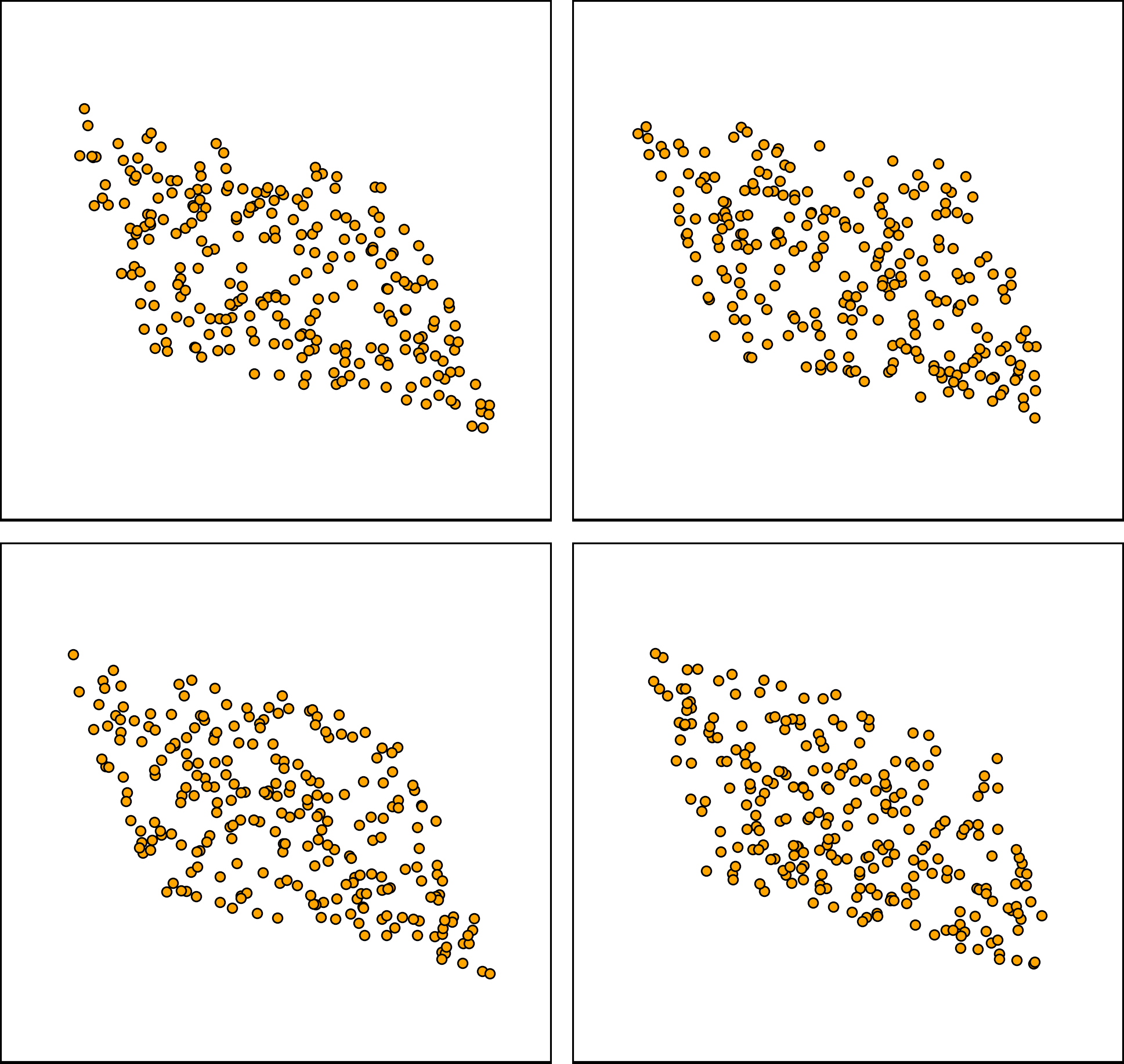
Figure 1: Barycenter of location-scatter Swiss roll population computed by three methods.

In this section, we consider N=4N=4 with (α1,…,α4)=(0.1,0.2,0.3,0.4)(\alpha_{1},\dots,\alpha_{4})=(0.1,0.2,0.3,0.4) as weights. We consider the location-scatter family of distributions (Álvarez-Esteban et al. 2016, §4) whose true barycenter can be computed. Let ℙ0∈𝒫2,ac\mathbb{P}_{0}\in\mathcal{P}_{2,\text{ac}} and define the following location-scatter family of distributions ℱ(ℙ0)={fS,u♯ℙ0 | S∈ℳD×D+,u∈ℝD},\mathcal{F}(\mathbb{P}_{0})=\{f_{S,u}\sharp\mathbb{P}_{0}\mbox{ }|\mbox{ }S\in\mathcal{M}^{+}_{D\times D},u\in\mathbb{R}^{D}\}, where fS,u:ℝD→ℝDf_{S,u}:\mathbb{R}^{D}\rightarrow\mathbb{R}^{D} is a linear map fS,u​(x)=S​x+uf_{S,u}(x)=Sx+u with positive definite matrix S∈ℳD×D+S\in\mathcal{M}^{+}_{D\times D}. When {ℙn}⊂ℱ⁡(ℙ0)\{\mathbb{P}_{n}\}\subset\mathcal{F}(\mathbb{P}_{0}), their barycenter ℙ¯\overline{\mathbb{P}} is also an element of ℱ⁡(ℙ0)\mathcal{F}(\mathbb{P}_{0}) and can be computed via fixed-point iterations (Álvarez-Esteban et al. 2016).

Figure 1(a) shows a 2-dimensional location-scatter family generated by using the Swiss roll distribution as ℙ0\mathbb{P}_{0}. The true barycenter is shown in Figure 1(b). The generated barycenter g​♯​𝕊g\sharp\mathbb{S} of [SC𝕎2\mathbb{W}_{2}B] is given in Figure 1(c). The pushforward measures ∇ψn†♯ℙn\nabla\psi_{n}^{\dagger}\sharp\mathbb{P}_{n} of each method are provided in Figures 1(d), 1(e), 1(f), respectively. In this example, the pushforward measures ∇ψn♯ℙn\nabla\psi_{n}\sharp\mathbb{P}_{n} all reasonably approximate ℙ¯\overline{\mathbb{P}}, whereas the generated barycenter g​♯​𝕊g\sharp\mathbb{S} of [SC𝕎2\mathbb{W}_{2}B] (Figure 1(c)) visibly underfits.

For quantitative comparison, we consider two choices for ℙ0\mathbb{P}_{0}: the DD-dimensional standard Gaussian distribution and the uniform distribution on [−3,+3]D[-\sqrt{3},+\sqrt{3}]^{D}. Each ℙn\mathbb{P}_{n} is constructed as fSnT​Λ​Sn,0​♯​ℙ0∈ℱ⁡(ℙ0)f_{S_{n}^{T}\Lambda S_{n},0}\sharp\mathbb{P}_{0}\in\mathcal{F}(\mathbb{P}_{0}), where SnS_{n} is a random rotation matrix and Λ\Lambda is diagonal with entries [12​b0,12​b1,…,2][\frac{1}{2}b^{0},\frac{1}{2}b^{1},\dots,2] where b=4D−1b=\sqrt[D-1]{4}. We consider only centered distributions (i.e. zero mean) because the barycenter of non-centered {ℙn}∈𝒫2,ac​(ℝD){\{\mathbb{P}_{n}\}\in\mathcal{P}_{2,\text{ac}}(\mathbb{R}^{D})} is the barycenter of {ℙn′}\{\mathbb{P}_{n}^{\prime}\} shifted by ∑n=1Nαn​μℙn\sum_{n=1}^{N}\alpha_{n}\mu_{\mathbb{P}_{n}}, where {ℙn′}\{\mathbb{P}_{n}^{\prime}\} are centered copies of {ℙn}\{\mathbb{P}_{n}\} (Álvarez-Esteban et al. 2016). Results are shown in Table 1 and 2.

Metric Method D=2 4 8 16 32 64 128 256
B𝕎22\mathbb{W}_{2}^{2}-UVP, % [FC𝕎\mathbb{W}B], Cuturi & Doucet 2014 0.7 0.68 1.41 3.87 8.85 14.08 18.11 21.33
[SC𝕎2\mathbb{W}_{2}B], (Fan et al. 2020) 0.07 0.09 0.16 0.28 0.43 0.59 1.28 2.85
ℒ2\mathcal{L}_{2}-UVP, % (potentials) 0.08 0.10 0.17 0.29 0.47 0.63 1.14 1.50
[CR𝕎\mathbb{W}B], (Li et al. 2020) 0.99 2.52 8.62 22.23 67.01 >100
[C𝕎2\mathbb{W}_{2}B], ours 0.06 0.05 0.07 0.11 0.19 0.24 0.42 0.83
Table 1: Comparison of UVP for the case {ℙn}⊂ℱ⁡(ℙ0)\{\mathbb{P}_{n}\}\subset\mathcal{F}(\mathbb{P}_{0}), ℙ0=𝒩⁡(0,ID){\mathbb{P}_{0}=\mathcal{N}(0,I_{D})}, N=4N=4.
Metric Method D=2 4 8 16 32 64 128 256
B𝕎22\mathbb{W}_{2}^{2}-UVP, % [FC𝕎\mathbb{W}B], Cuturi & Doucet 2014 0.64 0.77 1.22 3.75 8.92 14.3 18.46 21.64
[SC𝕎2\mathbb{W}_{2}B], (Fan et al. 2020) 0.120.12 0.100.10 0.190.19 0.290.29 0.460.46 0.60.6 1.381.38 2.92.9
ℒ2\mathcal{L}_{2}-UVP, % (potentials) 0.170.17 0.120.12 0.20.2 0.310.31 0.470.47 0.620.62 1.211.21 1.521.52
[CR𝕎\mathbb{W}B], (Li et al. 2020) 0.580.58 1.831.83 8.098.09 21.2321.23 55.1755.17 >100>100
[C𝕎2\mathbb{W}_{2}B], ours 0.170.17 0.080.08 0.060.06 0.10.1 0.20.2 0.250.25 0.420.42 0.820.82
Table 2: Comparison of UVP for the case {ℙn}⊂ℱ⁡(ℙ0)\{\mathbb{P}_{n}\}\subset\mathcal{F}(\mathbb{P}_{0}), ℙ0=Uniform​([−3,+3]D){\mathbb{P}_{0}=\text{Uniform}\big([-\sqrt{3},+\sqrt{3}]^{D}}\big), N=4N=4.

In these experiments, our method outperforms [CR𝕎\mathbb{W}B] and [SC𝕎2\mathbb{W}_{2}B]. For [CR𝕎\mathbb{W}B], dimension ∼16\sim\!16 is the breakpoint: the method does not scale well to higher dimensions. [SC𝕎2\mathbb{W}_{2}B] scales with the increasing dimension better, but its errors ℒ2\mathcal{L}^{2}-UVP and B𝕎22\mathbb{W}_{2}^{2}-UVP are twice as high as ours. This is likely due to the generative approximation and the difficult min-max-min optimization in [SC𝕎2\mathbb{W}_{2}B]. For completeness, we also compare our algorithm to the proposed in Cuturi & Doucet 2014 which approximates the barycenter by a discrete distribution on a fixed number of free-support points. In our experiment, similar to Li et al. 2020, we set 50005000 as the support size. As expected, the B𝕎22\mathbb{W}_{2}^{2}-UVP error of the method increases drastically as the dimension grows and the method is outperformed by our approach.

To show the scalability of our method with the number of input distributions NN, we conduct an analogous experiment with a high-dimensional location-scatter family for N=20N=20. We set αn=2​nN⁡(N+1){\alpha_{n}=\frac{2n}{N(N+1)}} for n=1,2,…,20n=1,2,...,20 and choose the uniform distribution on [−3,+3]D[-\sqrt{3},+\sqrt{3}]^{D} as ℙ0\mathbb{P}_{0} and construct distributions ℙn∈ℱ⁡(ℙ0)\mathbb{P}_{n}\in\mathcal{F}(\mathbb{P}_{0}) as before. The results for dimensions 32, 64 and 128 are provided in Table 3. Similar to the results from Tables 1 and 2, we see that our method outperforms the alternatives.

Metric Method D=32 64 128
B𝕎22\mathbb{W}_{2}^{2}-UVP, % [FC𝕎\mathbb{W}B], Cuturi & Doucet 2014 14.09 26.21 38.43
[SC𝕎2\mathbb{W}_{2}B], (Fan et al. 2020) 0.620.62 0.930.93 1.831.83
ℒ2\mathcal{L}_{2}-UVP, % (potentials) 0.600.60 0.860.86 1.521.52
[C𝕎2\mathbb{W}_{2}B], ours 0.310.31 0.580.58 1.451.45
Table 3: Comparison of UVP for the case {ℙn}⊂ℱ⁡(ℙ0)\{\mathbb{P}_{n}\}\subset\mathcal{F}(\mathbb{P}_{0}), ℙ0=Uniform​([−3,+3]D){\mathbb{P}_{0}=\text{Uniform}\big([-\sqrt{3},+\sqrt{3}]^{D}}\big), N=20N=20.

5.2 Subset Posterior Aggregation

We apply our method to aggregate subset posterior distributions. The barycenter of subset posteriors converges to the true posterior (Srivastava et al. 2018). Thus, computing the barycenter of subset posteriors is an efficient alternative to obtaining a full posterior in the big data setting (Srivastava et al. 2015; Staib et al. 2017; Li et al. 2020).

Analogous to (Li et al. 2020), we consider Poisson and negative binomial regressions for predicting the hourly number of bike rentals using features such as the day of the week and weather conditions.22 2 http://archive.ics.uci.edu/ml/datasets/Bike+Sharing+Dataset We consider the posterior on the 8-dimensional regression coefficients for both Poisson and negative binomial regressions. We randomly split the data into N=5N=5 equally-sized subsets and obtain 10510^{5} samples from each subset posterior using the Stan library (Carpenter et al. 2017). This gives the discrete uniform distributions {ℙn}\{\mathbb{P}_{n}\} supported on the samples. As the ground truth barycenter ℙ¯\overline{\mathbb{P}}, we consider the full dataset posterior also consisting of 10510^{5} points.

We use B𝕎22\mathbb{W}_{2}^{2}-UVP(ℙ~,ℙ¯)(\tilde{\mathbb{P}},\overline{\mathbb{P}}) to compare the estimated barycenter ℙ~\tilde{\mathbb{P}} (pushforward measure ∇ψ†n♯ℙn\nabla\psi^{\dagger}_{n}\sharp\mathbb{P}_{n} or generated measure g​♯​𝕊g\sharp\mathbb{S}) with the true barycenter. The results are in Table 4. All considered methods perform well (UVP<2%<2\%), but our method outperforms the alternatives.

Regression SC𝕎2\mathbb{W}_{2}B, (Fan et al. 2020) [CR𝕎\mathbb{W}B], (Li et al. 2020) C𝕎2\mathbb{W}_{2}B, ours
ℙ~=g​♯​𝕊\tilde{\mathbb{P}}=g\sharp\mathbb{S} ℙ~=∇ψn♯ℙn\tilde{\mathbb{P}}=\nabla\psi_{n}\sharp\mathbb{P}_{n}
B𝕎22\mathbb{W}_{2}^{2}-UVP, % Poisson 0.670.67 0.410.41 1.531.53 0.10.1
negative binomial 0.150.15 0.150.15 1.261.26 0.110.11
Table 4: Comparison of UVP for recovered barycenters in our subset posterior aggregation task.

5.3 Color Palette Averaging

For qualitative study, we apply our method to aggregating color palettes of images. For an RGB image ℐ\mathcal{I}, its color palette is defined by the discrete uniform distribution ℙ⁡(ℐ)\mathbb{P}(\mathcal{I}) of all its pixels ∈[0,1]3\in[0,1]^{3}. For 33 images {ℐn}\{\mathcal{I}_{n}\} we compute the barycenter ℙ¯\overline{\mathbb{P}} of each color palette ℙn=ℙ⁡(ℐn)\mathbb{P}_{n}=\mathbb{P}(\mathcal{I}_{n}) w.r.t. uniform weights αn=13\alpha_{n}=\frac{1}{3}. We apply each computed potential ∇ψn†\nabla\psi^{\dagger}_{n} pixel-wise to ℐn\mathcal{I}_{n} to obtain the “pushforward” image ∇ψ†n♯ℐn\nabla\psi^{\dagger}_{n}\sharp\mathcal{I}_{n}. These “pushforward” images should be close to the barycenter ℙ¯\overline{\mathbb{P}} of {ℙn}\{\mathbb{P}_{n}\}.

Refer to caption
(a) Original images {ℐn}\{\mathcal{I}_{n}\}.
Refer to caption
(b) Color palettes {ℙn}\{\mathbb{P}_{n}\} of original images.
Refer to caption
(c) Images with averaged color palette {∇ψn†♯ℐn}\{\nabla\psi^{\dagger}_{n}\sharp\mathcal{I}_{n}\}.
Refer to caption
(d) Barycenter palettes {∇ψn†♯ℙn}\{\nabla\psi^{\dagger}_{n}\sharp\mathbb{P}_{n}\}.
Figure 2: Results of our method applied to averaging color palettes of images.

The results are provided in Figure 2. Note that the image ∇ψ†1♯ℐ1\nabla\psi^{\dagger}_{1}\sharp\mathcal{I}_{1} inherits certain attributes of images ℐ2\mathcal{I}_{2} and ℐ3\mathcal{I}_{3}: the sky becomes bluer and the trees becomes greener. On the other hand, the sunlight in images ∇ψ†2♯ℐ2,∇ψ†3♯ℐ3\nabla\psi^{\dagger}_{2}\sharp\mathcal{I}_{2},\nabla\psi^{\dagger}_{3}\sharp\mathcal{I}_{3} has acquired an orange tint, thanks to the dominance of orange in ℐ1\mathcal{I}_{1}.

Acknowledgments

The Skoltech Advanced Data Analytics in Science and Engineering Group thanks the Skoltech CDISE HPC Zhores cluster staff for computing cluster provision and Skoltech-MIT NGP initiative for the support.

The MIT Geometric Data Processing group acknowledges the generous support of Army Research Office grant W911NF2010168, of Air Force Office of Scientific Research award FA9550-19-1-031, of National Science Foundation grant IIS-1838071, from the CSAIL Systems that Learn program, from the MIT–IBM Watson AI Laboratory, from the Toyota–CSAIL Joint Research Center, from a gift from Adobe Systems, from an MIT.nano Immersion Lab/NCSOFT Gaming Program seed grant, and from the Skoltech–MIT Next Generation Program.

References

  • Agueh & Carlier (2011) Martial Agueh and Guillaume Carlier. Barycenters in the wasserstein space. SIAM Journal on Mathematical Analysis, 43(2):904–924, 2011.
  • Álvarez-Esteban et al. (2016) Pedro C Álvarez-Esteban, E Del Barrio, JA Cuesta-Albertos, and C Matrán. A fixed-point approach to barycenters in wasserstein space. Journal of Mathematical Analysis and Applications, 441(2):744–762, 2016.
  • Amos et al. (2017) Brandon Amos, Lei Xu, and J Zico Kolter. Input convex neural networks. In Proceedings of the 34th International Conference on Machine Learning-Volume 70, pp. 146–155. JMLR. org, 2017.
  • Brenier (1991) Yann Brenier. Polar factorization and monotone rearrangement of vector-valued functions. Communications on pure and applied mathematics, 44(4):375–417, 1991.
  • Carpenter et al. (2017) Bob Carpenter, Andrew Gelman, Matthew D Hoffman, Daniel Lee, Ben Goodrich, Michael Betancourt, Marcus Brubaker, Jiqiang Guo, Peter Li, and Allen Riddell. Stan: A probabilistic programming language. Journal of statistical software, 76(1), 2017.
  • Chewi et al. (2020) Sinho Chewi, Tyler Maunu, Philippe Rigollet, and Austin J Stromme. Gradient descent algorithms for bures-wasserstein barycenters. arXiv preprint arXiv:2001.01700, 2020.
  • Cohen et al. (2020) Samuel Cohen, Michael Arbel, and Marc Peter Deisenroth. Estimating barycenters of measures in high dimensions. arXiv preprint arXiv:2007.07105, 2020.
  • Cuturi (2013) Marco Cuturi. Sinkhorn distances: Lightspeed computation of optimal transport. In Advances in neural information processing systems, pp. 2292–2300, 2013.
  • Cuturi & Doucet (2014) Marco Cuturi and Arnaud Doucet. Fast computation of wasserstein barycenters. 2014.
  • Dowson & Landau (1982) DC Dowson and BV Landau. The fréchet distance between multivariate normal distributions. Journal of multivariate analysis, 12(3):450–455, 1982.
  • Dvurechenskii et al. (2018) Pavel Dvurechenskii, Darina Dvinskikh, Alexander Gasnikov, Cesar Uribe, and Angelia Nedich. Decentralize and randomize: Faster algorithm for wasserstein barycenters. In Advances in Neural Information Processing Systems, pp. 10760–10770, 2018.
  • Fan et al. (2020) Jiaojiao Fan, Amirhossein Taghvaei, and Yongxin Chen. Scalable computations of wasserstein barycenter via input convex neural networks. arXiv preprint arXiv:2007.04462, 2020.
  • Fenchel (1949) Werner Fenchel. On conjugate convex functions. Canadian Journal of Mathematics, 1(1):73–77, 1949.
  • Genevay et al. (2016) Aude Genevay, Marco Cuturi, Gabriel Peyré, and Francis Bach. Stochastic optimization for large-scale optimal transport. In Advances in neural information processing systems, pp. 3440–3448, 2016.
  • Kakade et al. (2009) Sham Kakade, Shai Shalev-Shwartz, and Ambuj Tewari. On the duality of strong convexity and strong smoothness: Learning applications and matrix regularization. Unpublished Manuscript, http://ttic. uchicago. edu/shai/papers/KakadeShalevTewari09. pdf, 2(1), 2009.
  • Kantorovitch (1958) Leonid Kantorovitch. On the translocation of masses. Management Science, 5(1):1–4, 1958.
  • Kingma & Ba (2014) Diederik P Kingma and Jimmy Ba. Adam: A method for stochastic optimization. arXiv preprint arXiv:1412.6980, 2014.
  • Korotin et al. (2019a) Alexander Korotin, Vage Egiazarian, Arip Asadulaev, Alexander Safin, and Evgeny Burnaev. Wasserstein-2 generative networks. arXiv preprint arXiv:1909.13082, 2019a.
  • Korotin et al. (2019b) Alexander Korotin, Vladimir V’yugin, and Evgeny Burnaev. Integral mixability: a tool for efficient online aggregation of functional and probabilistic forecasts. arXiv preprint arXiv:1912.07048, 2019b.
  • Li et al. (2020) Lingxiao Li, Aude Genevay, Mikhail Yurochkin, and Justin Solomon. Continuous regularized wasserstein barycenters. arXiv preprint arXiv:2008.12534, 2020.
  • Makkuva et al. (2019) Ashok Vardhan Makkuva, Amirhossein Taghvaei, Sewoong Oh, and Jason D Lee. Optimal transport mapping via input convex neural networks. arXiv preprint arXiv:1908.10962, 2019.
  • McCann et al. (1995) Robert J McCann et al. Existence and uniqueness of monotone measure-preserving maps. Duke Mathematical Journal, 80(2):309–324, 1995.
  • Mroueh (2019) Youssef Mroueh. Wasserstein style transfer. arXiv preprint arXiv:1905.12828, 2019.
  • Pearlmutter (1994) Barak A Pearlmutter. Fast exact multiplication by the hessian. Neural computation, 6(1):147–160, 1994.
  • Peyré et al. (2019) Gabriel Peyré, Marco Cuturi, et al. Computational optimal transport. Foundations and Trends® in Machine Learning, 11(5-6):355–607, 2019.
  • Rabin et al. (2011) Julien Rabin, Gabriel Peyré, Julie Delon, and Marc Bernot. Wasserstein barycenter and its application to texture mixing. In International Conference on Scale Space and Variational Methods in Computer Vision, pp. 435–446. Springer, 2011.
  • Rabin et al. (2014) Julien Rabin, Sira Ferradans, and Nicolas Papadakis. Adaptive color transfer with relaxed optimal transport. In 2014 IEEE International Conference on Image Processing (ICIP), pp. 4852–4856. IEEE, 2014.
  • Seguy et al. (2017) Vivien Seguy, Bharath Bhushan Damodaran, Rémi Flamary, Nicolas Courty, Antoine Rolet, and Mathieu Blondel. Large-scale optimal transport and mapping estimation. arXiv preprint arXiv:1711.02283, 2017.
  • Solomon et al. (2015) Justin Solomon, Fernando De Goes, Gabriel Peyré, Marco Cuturi, Adrian Butscher, Andy Nguyen, Tao Du, and Leonidas Guibas. Convolutional wasserstein distances: Efficient optimal transportation on geometric domains. ACM Transactions on Graphics (TOG), 34(4):1–11, 2015.
  • Srivastava et al. (2015) Sanvesh Srivastava, Volkan Cevher, Quoc Dinh, and David Dunson. Wasp: Scalable bayes via barycenters of subset posteriors. In Artificial Intelligence and Statistics, pp. 912–920, 2015.
  • Srivastava et al. (2018) Sanvesh Srivastava, Cheng Li, and David B Dunson. Scalable bayes via barycenter in wasserstein space. The Journal of Machine Learning Research, 19(1):312–346, 2018.
  • Staib et al. (2017) Matthew Staib, Sebastian Claici, Justin M Solomon, and Stefanie Jegelka. Parallel streaming Wasserstein barycenters. In Advances in Neural Information Processing Systems, pp. 2647–2658, 2017.
  • Villani (2003) Cédric Villani. Topics in optimal transportation. Number 58. American Mathematical Soc., 2003.
  • Weed et al. (2019) Jonathan Weed, Francis Bach, et al. Sharp asymptotic and finite-sample rates of convergence of empirical measures in wasserstein distance. Bernoulli, 25(4A):2620–2648, 2019.
  • Xie et al. (2019) Yujia Xie, Minshuo Chen, Haoming Jiang, Tuo Zhao, and Hongyuan Zha. On scalable and efficient computation of large scale optimal transport. volume 97 of Proceedings of Machine Learning Research, pp. 6882–6892, Long Beach, California, USA, 09–15 Jun 2019. PMLR. URL http://proceedings.mlr.press/v97/xie19a.html.

Appendix A The Algorithm

The numerical procedure for solving our final objective (14) is given below.

Input : Distributions ℙ1,…,ℙN\mathbb{P}_{1},\dots,\mathbb{P}_{N} with sample access;
Weights α1,…,αN≥0\alpha_{1},\dots,\alpha_{N}\geq 0 with ∑n=1Nαn=1\sum_{n=1}^{N}\alpha_{n}=1;
Regularization distribution ℙ^′\widehat{\mathbb{P}}^{\prime} given by a sampler;
Congruence regularizer coefficient τ≥1\tau\geq 1;
Balancing coefficient γ∈[0,1]\gamma\in[0,1];
Cycle-consistency regularizer coefficient λ>0\lambda>0;
2​N2N ICNNs {ψθn,ψωn¯}\{\psi_{\theta_{n}},\overline{\psi_{\omega_{n}}}\};
Batch size K>0K>0;
for t=1,2,…t=1,2,\dots do
1. Sample batches Xn∼ℙnX_{n}\sim\mathbb{P}_{n} for all n=1,…,Nn=1,\dots,N;
    2. Compute the pushforwards Yn=∇ψθn♯XnY_{n}=\nabla\psi_{\theta_{n}}\sharp X_{n} for all n=1,…,Nn=1,\dots,N;
    3. Sample batch Y0∼ℙ^Y_{0}\sim\widehat{\mathbb{P}};
    4. Compute the Monte-Carlo estimate of the congruence regularizer:
ℒCongruence:=1K⋅∑n=1Nγn​∑y∈Yn[∑n′=1Nαn′​ψωn′¯​(y)−‖y‖22]+,\mathcal{L}_{\text{Congruence}}:=\frac{1}{K}\cdot\sum_{n=1}^{N}\gamma_{n}\sum_{y\in Y_{n}}\big[\sum_{n^{\prime}=1}^{N}\alpha_{n^{\prime}}\overline{\psi_{\omega_{n^{\prime}}}}(y)-\frac{\|y\|^{2}}{2}\big]_{+},
where γ0=γ\gamma_{0}=\gamma and γn=αn⋅(1−γ)\gamma_{n}=\alpha_{n}\cdot(1-\gamma) for n=1,2,…,Nn=1,2,\dots,N;
    5. Compute the Monte-Carlo estimate of the cycle-consistency regularizer:
ℒCycle:=1K​∑n=1Nαn​[∑x∈Xn‖∇ψωn¯∘∇ψθn​(x)−x‖22];\mathcal{L}_{\text{Cycle}}:=\frac{1}{K}\sum_{n=1}^{N}\alpha_{n}\bigg[\sum_{x\in X_{n}}\|\nabla\overline{\psi_{\omega_{n}}}\circ\nabla\psi_{\theta_{n}}(x)-x\|_{2}^{2}\bigg];
6. Compute the Monte-Carlo estimate of multiple correlations:
ℒMultiCorr:=∑n=1N[αn⋅1K∑x∈Xn[⟨x,∇ψθn(x)⟩−ψωn¯(∇ψθn(x))]];\mathcal{L}_{\text{MultiCorr}}:=\sum_{n=1}^{N}\bigg[\alpha_{n}\cdot\frac{1}{K}\sum_{x\in X_{n}}\big[\langle x,\nabla\psi_{\theta_{n}}(x)\rangle-\overline{\psi_{\omega_{n}}}(\nabla\psi_{\theta_{n}}(x))]\bigg];
7. Compute the total loss:
ℒTotal:=ℒMultiCorr+λ⋅ℒCycle+τ⋅ℒCongruence;\mathcal{L}_{\text{Total}}:=\mathcal{L}_{\text{MultiCorr}}+\lambda\cdot\mathcal{L}_{\text{Cycle}}+\tau\cdot\mathcal{L}_{\text{Congruence}};
8. Perform a gradient step over {θn,ωn}\{\theta_{n},\omega_{n}\} by using ∂ℒTotal∂{θn,ωn}\frac{\partial\mathcal{L}_{\text{Total}}}{\partial\{\theta_{n},\omega_{n}\}};
    end for
Algorithm 1 Numerical Procedure for Optimizing Multiple Correlations (14)

Parametrization of the potentials. To parametrize potentials {ψθn,ψωn¯}\{\psi_{\theta_{n}},\overline{\psi_{\omega_{n}}}\}, we use DenseICNN (dense input convex neural network) with quadratic skip connections; see (Korotin et al. 2019a, Appendix B.2). As an initialization step, we pre-train the potentials to satisfy

ψθn​(x)≈‖x‖22andψωn¯​(y)≈‖y‖22.\psi_{\theta_{n}}(x)\approx\frac{\|x\|^{2}}{2}\qquad\text{and}\qquad\overline{\psi_{\omega_{n}}}(y)\approx\frac{\|y\|^{2}}{2}.

Such pre-training provides a good start for the networks: each ψθn\psi_{\theta_{n}} is approximately conjugate to the corresponding ψωn¯\overline{\psi_{\omega_{n}}}. On the other hand, the initial networks {ψθn}\{\psi_{\theta_{n}}\} are approximate congruent according to (5).

Computational Complexity. For a single training iteration, the time complexity of both forward (evaluation) and backward (computing the gradient with respect to the parameters) passes through the objective function (14) is O⁡(N​T)O(NT). Here NN is the number of input distributions and TT is the time taken by evaluating each individual potential (parameterized as a neural network) on a batch of points sampled from either ℙn\mathbb{P}_{n} or ℙ^\widehat{\mathbb{P}}. This claim follows from the well-known fact that gradient evaluation ∇θhθ​(x)\nabla_{\theta}h_{\theta}(x) of hθ:ℝD→ℝh_{\theta}:\mathbb{R}^{D}\to\mathbb{R}, when parameterized as a neural network, requires time proportional to the size of the computational graph. Hence, gradient computation requires computational time proportional to the time for evaluating the function hθ​(x)h_{\theta}(x) itself. The same holds when computing the derivative with respect to xx. Then, for instance, computing the term ∇ψn‡¯∘∇ψn†​(x)\nabla\overline{\psi_{n}^{\ddagger}}\circ\nabla\psi_{n}^{\dagger}(x) in (14) takes O⁡(T)O(T) time. The gradient of this term with respect to θ\theta also takes O⁡(T)O(T) time: Hessian-vector products that appear can be calculated in O⁡(T)O(T) time using the famous Hessian trick, see Pearlmutter 1994.

In practice, we compute all the gradients using automatic differentiation. We empirically measured that for our DenseICNN potentials, the computation of their gradient w.r.t. input xx, i.e., ∇ψ†​(x)\nabla\psi^{\dagger}(x), requires roughly 3-4x more time than the computation of ψ†​(x)\psi^{\dagger}(x).

Appendix B Proofs

In this section, we prove our main Theorems 4.1 and 4.2.

We use ℒ2(ℝD→ℝD,μ)\mathcal{L}^{2}(\mathbb{R}^{D}\rightarrow\mathbb{R}^{D},\mu) to denote the Hilbert space of functions f:ℝD→ℝD{f:\mathbb{R}^{D}\rightarrow\mathbb{R}^{D}} with integrable square w.r.t. a probability measure μ\mu. The corresponding inner product for f1,f2∈ℒ2(ℝD→ℝD,μ)f_{1},f_{2}\in\mathcal{L}^{2}(\mathbb{R}^{D}\rightarrow\mathbb{R}^{D},\mu) is denoted by

⟨f1,f2⟩μ=def∫ℝD⟨f1​(x),f2​(x)⟩​𝑑μ​(x),\langle f_{1},f_{2}\rangle_{\mu}\stackrel{{\scriptstyle\text{def}}}{{=}}\int_{\mathbb{R}^{D}}\langle f_{1}(x),f_{2}(x)\rangle d\mu(x),

where ⟨f1​(x),f2​(x)⟩\langle f_{1}(x),f_{2}(x)\rangle is the Euclidean dot product. We use ∥⋅∥μ=⟨⋅,⋅⟩μ\|\cdot\|_{\mu}=\sqrt{\langle\cdot,\cdot\rangle_{\mu}} to denote the norm induced by the inner product in ℒ2(ℝD→ℝD,μ)\mathcal{L}^{2}(\mathbb{R}^{D}\rightarrow\mathbb{R}^{D},\mu).

We also recall a useful property of lower semi-continuous convex function ψ:ℝD→ℝ\psi:\mathbb{R}^{D}\rightarrow\mathbb{R}:

∇ψ​(x)=arg​maxy∈ℝD⁡[⟨y,x⟩−ψ¯​(y)],\nabla\psi(x)=\argmax_{y\in\mathbb{R}^{D}}\big[\langle y,x\rangle-\overline{\psi}(y)\big], (19)

which follows from the fact that

y^=arg​maxy∈ℝD⁡[⟨y,x⟩−ψ¯​(y)]⇔x−∇ψ¯​(y^)=0.\hat{y}=\argmax_{y\in\mathbb{R}^{D}}\big[\langle y,x\rangle-\overline{\psi}(y)\big]\iff x-\nabla\overline{\psi}(\hat{y})=0.

We begin with the proof of Theorem 4.1.

Proof.

We consider the difference between the estimated correlations and true ones:

Δ=∑n=1Nαn​∫ℝDψn​(x)​d​ℙn​(x)−∑n=1Nαn​∫ℝDψn∗​(x)​d​ℙn​(x)=\displaystyle\Delta=\sum_{n=1}^{N}\alpha_{n}\int_{\mathbb{R}^{D}}\psi_{n}(x)d\mathbb{P}_{n}(x)-\sum_{n=1}^{N}\alpha_{n}\int_{\mathbb{R}^{D}}\psi_{n}^{*}(x)d\mathbb{P}_{n}(x)=
∑n=1Nαn​∫ℝD[⟨∇ψn​(x),x⟩−ψn¯​(∇ψn​(x))]​d​ℙn​(x)−\displaystyle\sum_{n=1}^{N}\alpha_{n}\int_{\mathbb{R}^{D}}\big[\langle\nabla\psi_{n}(x),x\rangle-\overline{\psi_{n}}\big(\nabla\psi_{n}(x))\big]d\mathbb{P}_{n}(x)-
∑n=1Nαn​∫ℝD[⟨∇ψn∗​(x),x⟩−ψn∗¯​(∇ψn∗​(x))]​d​ℙn​(x),\displaystyle\sum_{n=1}^{N}\alpha_{n}\int_{\mathbb{R}^{D}}\big[\langle\nabla\psi_{n}^{*}(x),x\rangle-\overline{\psi_{n}^{*}}\big(\nabla\psi_{n}^{*}(x))\big]d\mathbb{P}_{n}(x), (20)

where we twice use (19) for f=ψnf=\psi_{n} and f=ψn∗f=\psi^{*}_{n}. We note that

∑n=1Nαn​∫ℝD⟨∇ψn∗​(x),x⟩​d​ℙn​(x)=∑n=1Nαn​∫ℝD⟨y,∇ψn∗¯​(y)⟩​𝑑ℙ¯​(y)=\displaystyle\sum_{n=1}^{N}\alpha_{n}\int_{\mathbb{R}^{D}}\langle\nabla\psi_{n}^{*}(x),x\rangle d\mathbb{P}_{n}(x)=\sum_{n=1}^{N}\alpha_{n}\int_{\mathbb{R}^{D}}\langle y,\nabla\overline{\psi_{n}^{*}}(y)\rangle d\overline{\mathbb{P}}(y)=
∫ℝD⟨y,∑n=1Nαn∇ψn∗¯(y)⟩dℙ¯(y)=∫ℝD⟨y,y⟩dℙ¯(y)=∥idℝD∥ℙ¯2,\displaystyle\int_{\mathbb{R}^{D}}\langle y,\sum_{n=1}^{N}\alpha_{n}\nabla\overline{\psi_{n}^{*}}(y)\rangle d\overline{\mathbb{P}}(y)=\int_{\mathbb{R}^{D}}\langle y,y\rangle d\overline{\mathbb{P}}(y)=\|\text{id}_{\mathbb{R}^{D}}\|_{\overline{\mathbb{P}}}^{2}, (21)

where we use of change-of-variable formula for ∇ψn∗♯ℙn=ℙ¯\nabla\psi_{n}^{*}\sharp\mathbb{P}_{n}=\overline{\mathbb{P}} and (5). Analogously,

∑n=1Nαn​∫ℝDψn∗¯​(∇ψn∗​(x))​d​ℙn​(x)=∑n=1Nαn​∫ℝDψn∗¯​(y)​𝑑ℙ¯​(y)=\displaystyle\sum_{n=1}^{N}\alpha_{n}\int_{\mathbb{R}^{D}}\overline{\psi_{n}^{*}}\big(\nabla\psi_{n}^{*}(x))d\mathbb{P}_{n}(x)=\sum_{n=1}^{N}\alpha_{n}\int_{\mathbb{R}^{D}}\overline{\psi_{n}^{*}}\big(y)d\overline{\mathbb{P}}(y)=
∫ℝD∑n=1Nαn​ψn∗¯​(y)​𝑑ℙ¯​(y)=∫ℝD‖y‖22​𝑑ℙ¯​(y)=12​‖idℝD‖ℙ¯2.\displaystyle\int_{\mathbb{R}^{D}}\sum_{n=1}^{N}\alpha_{n}\overline{\psi_{n}^{*}}\big(y)d\overline{\mathbb{P}}(y)=\int_{\mathbb{R}^{D}}\frac{\|y\|^{2}}{2}d\overline{\mathbb{P}}(y)=\frac{1}{2}\|\text{id}_{\mathbb{R}^{D}}\|_{\overline{\mathbb{P}}}^{2}. (22)

Since each ψn\psi_{n} is ℬ\mathcal{B}-smooth, we conclude that ψn¯\overline{\psi_{n}} is 1ℬ\frac{1}{\mathcal{B}}-strongly convex, see (Kakade et al. 2009). Thus, we have

OPENψn¯​(∇ψn∗​(x)))≥\displaystyle\overline{\psi_{n}}\big(\nabla\psi_{n}^{*}(x)))\geq
OPENψn¯​(∇ψn​(x)))+⟨∇ψn†¯∘∇ψn†​(x)⏟=x,∇ψn∗​(x)−∇ψn​(x)⟩+12​ℬ​‖∇ψn∗​(x)−∇ψn​(x)‖2=\displaystyle\overline{\psi_{n}}\big(\nabla\psi_{n}(x)))+\langle\underbrace{\nabla\overline{\psi_{n}^{\dagger}}\circ\nabla\psi_{n}^{\dagger}(x)}_{=x},\nabla\psi_{n}^{*}(x)-\nabla\psi_{n}(x)\rangle+\frac{1}{2\mathcal{B}}\|\nabla\psi_{n}^{*}(x)-\nabla\psi_{n}(x)\|^{2}=
OPENψn¯​(∇ψn​(x)))+⟨x,∇ψn∗​(x)−∇ψn​(x)⟩+12​ℬ​‖∇ψn∗​(x)−∇ψn​(x)‖2,\displaystyle\overline{\psi_{n}}\big(\nabla\psi_{n}(x)))+\langle x,\nabla\psi_{n}^{*}(x)-\nabla\psi_{n}(x)\rangle+\frac{1}{2\mathcal{B}}\|\nabla\psi_{n}^{*}(x)-\nabla\psi_{n}(x)\|^{2}, (23)

or equivalently

OPENOPEN−ψn¯​(∇ψn​(x)))≥−ψn¯​(∇ψn∗​(x)))+⟨x,∇ψn∗​(x)−∇ψn​(x)⟩+12​ℬ​‖∇ψn∗​(x)−∇ψn​(x)‖2.-\overline{\psi_{n}}\big(\nabla\psi_{n}(x)))\geq-\overline{\psi_{n}}\big(\nabla\psi_{n}^{*}(x)))+\langle x,\nabla\psi_{n}^{*}(x)-\nabla\psi_{n}(x)\rangle+\frac{1}{2\mathcal{B}}\|\nabla\psi_{n}^{*}(x)-\nabla\psi_{n}(x)\|^{2}. (24)

We integrate (24) w.r.t. ℙn\mathbb{P}_{n} and sum over n=1,2,…,Nn=1,2,\dots,N with weights αn\alpha_{n}:

−∑n=1Nαn∫ℝDψn¯(∇ψn(x))dℙn(x)≥\displaystyle-\sum_{n=1}^{N}\alpha_{n}\int_{\mathbb{R}^{D}}\overline{\psi_{n}}\big(\nabla\psi_{n}(x))d\mathbb{P}_{n}(x)\geq
−∑n=1Nαn∫ℝDψn¯(∇ψn∗(x))dℙn(x)+∑n=1Nαn⟨x,∇ψn∗(x)⟩ℙn−∑n=1Nαn⟨x,∇ψn(x)⟩ℙn+\displaystyle-\sum_{n=1}^{N}\alpha_{n}\int_{\mathbb{R}^{D}}\overline{\psi_{n}}\big(\nabla\psi_{n}^{*}(x))d\mathbb{P}_{n}(x)+\sum_{n=1}^{N}\alpha_{n}\langle x,\nabla\psi_{n}^{*}(x)\rangle_{\mathbb{P}_{n}}-\sum_{n=1}^{N}\alpha_{n}\langle x,\nabla\psi_{n}(x)\rangle_{\mathbb{P}_{n}}+
∑n=1Nαn​12​ℬ​‖∇ψn∗​(x)−∇ψn​(x)‖ℙn2=\displaystyle\sum_{n=1}^{N}\alpha_{n}\frac{1}{2\mathcal{B}}\|\nabla\psi_{n}^{*}(x)-\nabla\psi_{n}(x)\|^{2}_{\mathbb{P}_{n}}=
−∫ℝD∑n=1Nαnψn¯(y)dℙ¯(y)+∑n=1Nαn⟨x,∇ψn∗(x)⟩ℙn−\displaystyle-\int_{\mathbb{R}^{D}}\sum_{n=1}^{N}\alpha_{n}\overline{\psi_{n}}\big(y)d\overline{\mathbb{P}}(y)+\sum_{n=1}^{N}\alpha_{n}\langle x,\nabla\psi_{n}^{*}(x)\rangle_{\mathbb{P}_{n}}-
∑n=1Nαn​⟨x,∇ψn​(x)⟩ℙn+∑n=1Nαn​12​ℬ​‖∇ψn∗​(x)−∇ψn​(x)‖ℙn2.\displaystyle\sum_{n=1}^{N}\alpha_{n}\langle x,\nabla\psi_{n}(x)\rangle_{\mathbb{P}_{n}}+\sum_{n=1}^{N}\alpha_{n}\frac{1}{2\mathcal{B}}\|\nabla\psi_{n}^{*}(x)-\nabla\psi_{n}(x)\|^{2}_{\mathbb{P}_{n}}. (25)

We note that

−∫ℝD∑n=1Nαnψn¯(y)dℙ¯(y)=∫ℝD[‖y‖22−∑n=1Nαnψn¯(y)]dℙ¯(y)−∫ℝD‖y‖22dℙ¯(y)\displaystyle-\int_{\mathbb{R}^{D}}\sum_{n=1}^{N}\alpha_{n}\overline{\psi_{n}}\big(y)d\overline{\mathbb{P}}(y)=\int_{\mathbb{R}^{D}}\big[\frac{\|y\|^{2}}{2}-\sum_{n=1}^{N}\alpha_{n}\overline{\psi_{n}}\big(y)\big]d\overline{\mathbb{P}}(y)-\int_{\mathbb{R}^{D}}\frac{\|y\|^{2}}{2}d\overline{\mathbb{P}}(y)
∫ℝD[‖y‖22−∑n=1Nαn​ψn¯​(y)]​𝑑ℙ¯​(y)−12​‖idℝD‖ℙ¯2.\displaystyle\int_{\mathbb{R}^{D}}\big[\frac{\|y\|^{2}}{2}-\sum_{n=1}^{N}\alpha_{n}\overline{\psi_{n}}\big(y)\big]d\overline{\mathbb{P}}(y)-\frac{1}{2}\|\text{id}_{\mathbb{R}^{D}}\|_{\overline{\mathbb{P}}}^{2}. (26)

Now we substitute (25), (26), (21) and (22) into (20) to obtain (9). ∎

Next, we prove Theorem 4.2.

Proof.

Since ψn‡¯\overline{\psi_{n}^{\ddagger}} is β‡\beta^{\ddagger} strongly convex, its conjugate ψn‡\psi_{n}^{\ddagger} is 1β‡\frac{1}{\beta^{\ddagger}}-smooth, i.e. has 1β‡\frac{1}{\beta^{\ddagger}}-Lipschitz gradient ∇ψn‡\nabla\psi_{n}^{\ddagger} (Kakade et al. 2009). Thus, for all x,x′∈ℝDx,x^{\prime}\in\mathbb{R}^{D}:

‖∇ψn‡​(x)−∇ψn‡​(x′)‖2≤(1β‡)2⋅‖x−x′‖2.\|\nabla\psi_{n}^{\ddagger}(x)-\nabla\psi_{n}^{\ddagger}(x^{\prime})\|^{2}\leq(\frac{1}{\beta^{\ddagger}})^{2}\cdot\|x-x^{\prime}\|^{2}.

We substitute x′=∇ψn‡¯∘∇ψn†​(y)=(∇ψn‡)−1∘∇ψn†​(y)x^{\prime}=\nabla\overline{\psi_{n}^{\ddagger}}\circ\nabla\psi_{n}^{\dagger}(y)=\big(\nabla\psi_{n}^{\ddagger}\big)^{-1}\circ\nabla\psi_{n}^{\dagger}(y) and obtain:

‖∇ψn†​(x)−∇ψn‡​(x)‖2≤(1β‡)2​‖x−∇ψn‡¯∘∇ψn†​(x)‖2.\|\nabla\psi_{n}^{\dagger}(x)-\nabla\psi_{n}^{\ddagger}(x)\|^{2}\leq(\frac{1}{\beta^{\ddagger}})^{2}\|x-\nabla\overline{\psi_{n}^{\ddagger}}\circ\nabla\psi_{n}^{\dagger}(x)\|^{2}. (27)

Since the function ψn‡¯\overline{\psi_{n}^{\ddagger}} is ℬ‡\mathcal{B}^{\ddagger}-smooth, we have for all x∈ℝDx\in\mathbb{R}^{D}:

ψn‡¯​(∇ψn†​(x))≤ψn‡¯​(∇ψn‡​(x))+⟨∇ψn‡¯∘∇ψn‡​(x)⏟=x,∇ψn†​(x)−∇ψn‡​(x)⟩+ℬ‡2​‖∇ψn†​(x)−∇ψn‡​(x)‖2,\displaystyle\overline{\psi_{n}^{\ddagger}}(\nabla\psi_{n}^{\dagger}(x))\leq\overline{\psi_{n}^{\ddagger}}(\nabla\psi_{n}^{\ddagger}(x))+\langle\underbrace{\nabla\overline{\psi_{n}^{\ddagger}}\circ\nabla\psi_{n}^{\ddagger}(x)}_{=x},\nabla\psi_{n}^{\dagger}(x)-\nabla\psi_{n}^{\ddagger}(x)\rangle+\frac{\mathcal{B}^{\ddagger}}{2}\|\nabla\psi_{n}^{\dagger}(x)-\nabla\psi_{n}^{\ddagger}(x)\|^{2},

that is equivalent to:

⟨x,∇ψn†​(x)⟩−ψn‡¯​(∇ψn†​(x))≥⟨x,∇ψn‡​(x)⟩−ψn‡¯​(∇ψn‡​(x))⏟ψn‡​(x)−ℬ‡2​‖∇ψn†​(x)−∇ψn‡​(x)‖2.\displaystyle\langle x,\nabla\psi_{n}^{\dagger}(x)\rangle-\overline{\psi_{n}^{\ddagger}}(\nabla\psi_{n}^{\dagger}(x))\geq\underbrace{\langle x,\nabla\psi_{n}^{\ddagger}(x)\rangle-\overline{\psi_{n}^{\ddagger}}(\nabla\psi_{n}^{\ddagger}(x))}_{\psi^{\ddagger}_{n}(x)}-\frac{\mathcal{B}^{\ddagger}}{2}\|\nabla\psi_{n}^{\dagger}(x)-\nabla\psi_{n}^{\ddagger}(x)\|^{2}. (28)

We combine (28) with (27) to obtain

⟨x,∇ψn†​(x)⟩−ψn‡¯​(∇ψn†​(x))≥ψn‡​(x)−ℬ‡2​(β‡)2⋅‖idℝD−∇ψn‡¯∘∇ψn†‖2.\langle x,\nabla\psi_{n}^{\dagger}(x)\rangle-\overline{\psi_{n}^{\ddagger}}(\nabla\psi_{n}^{\dagger}(x))\geq\psi^{\ddagger}_{n}(x)-\frac{\mathcal{B}^{\ddagger}}{2(\beta^{\ddagger})^{2}}\cdot\|\text{id}_{\mathbb{R}^{D}}-\nabla\overline{\psi_{n}^{\ddagger}}\circ\nabla\psi_{n}^{\dagger}\|^{2}. (29)

For every n=1,2,…,Nn=1,2,\dots,N we integrate (29) w.r.t. ℙn\mathbb{P}_{n} and sum up the corresponding cycle-consistency regularization term:

∫ℝD[⟨x,∇ψn†​(x)⟩−ψn‡¯​(∇ψn†​(x))]​d​ℙn​(x)+λ⋅‖∇ψn‡¯∘∇ψn†−idℝD‖ℙn2≥\displaystyle\int_{\mathbb{R}^{D}}\big[\langle x,\nabla\psi_{n}^{\dagger}(x)\rangle-\overline{\psi_{n}^{\ddagger}}(\nabla\psi_{n}^{\dagger}(x))]d\mathbb{P}_{n}(x)+\lambda\cdot\|\nabla\overline{\psi_{n}^{\ddagger}}\circ\nabla\psi_{n}^{\dagger}-\text{id}_{\mathbb{R}^{D}}\|_{\mathbb{P}_{n}}^{2}\geq
∫ℝDψ‡​(x)​d​ℙn​(x)+(λ−ℬ†2​(β‡)2)⋅‖∇ψn‡¯∘∇ψn†−idℝD‖ℙn2⏟ℛ2ℙn​(ψn†,ψn‡¯).\displaystyle\int_{\mathbb{R}^{D}}\psi^{\ddagger}(x)d\mathbb{P}_{n}(x)+\big(\lambda-\frac{\mathcal{B}^{\dagger}}{2(\beta^{\ddagger})^{2}}\big)\cdot\underbrace{\|\nabla\overline{\psi_{n}^{\ddagger}}\circ\nabla\psi_{n}^{\dagger}-\text{id}_{\mathbb{R}^{D}}\|_{\mathbb{P}_{n}}^{2}}_{\mathcal{R}_{2}^{\mathbb{P}_{n}}(\psi_{n}^{\dagger},\overline{\psi_{n}^{\ddagger}})}. (30)

We sum (30) for n=1,2,…,Nn=1,2,\dots,N w.r.t. weights αn\alpha_{n} to obtain:

∑n=1Nαn​∫ℝD[⟨x,∇ψn†​(x)⟩−ψn‡¯​(∇ψn†​(x))]​d​ℙn​(x)+λ​∑n=1Nαn​ℛ2ℙn​(ψn†,ψn‡¯)≥\displaystyle\sum_{n=1}^{N}\alpha_{n}\int_{\mathbb{R}^{D}}\big[\langle x,\nabla\psi_{n}^{\dagger}(x)\rangle-\overline{\psi_{n}^{\ddagger}}(\nabla\psi_{n}^{\dagger}(x))]d\mathbb{P}_{n}(x)+\lambda\sum_{n=1}^{N}\alpha_{n}\mathcal{R}_{2}^{\mathbb{P}_{n}}(\psi_{n}^{\dagger},\overline{\psi_{n}^{\ddagger}})\geq
∑n=1Nαn​∫ℝDψ‡​(x)​d​ℙn​(x)⏟MultiCorr​({αn,ℙn}∣{ψn‡})+∑n=1Nαn​(λ−ℬ†2​(β‡)2)⋅ℛ2ℙn​(ψn†,ψn‡¯).\displaystyle\underbrace{\sum_{n=1}^{N}\alpha_{n}\int_{\mathbb{R}^{D}}\psi^{\ddagger}(x)d\mathbb{P}_{n}(x)}_{\text{MultiCorr}(\{\alpha_{n},\mathbb{P}_{n}\}\mid\{\psi^{\ddagger}_{n}\})}+\sum_{n=1}^{N}\alpha_{n}\big(\lambda-\frac{\mathcal{B}^{\dagger}}{2(\beta^{\ddagger})^{2}}\big)\cdot\mathcal{R}_{2}^{\mathbb{P}_{n}}(\psi_{n}^{\dagger},\overline{\psi_{n}^{\ddagger}}).

We add τ⋅ℛ1ℙ^​({ψn‡¯})\tau\cdot\mathcal{R}_{1}^{\widehat{{\mathbb{P}}}}(\{\overline{\psi_{n}^{\ddagger}}\}) to both sides of (B) to get

MultiCorr({αn,ℙn} | {ψn†},{ψn‡¯};τ,ℙ^,λ)≥MultiCorr({αn,ℙn}∣{ψn‡})+\displaystyle\text{MultiCorr}\big(\{\alpha_{n},\mathbb{P}_{n}\}\mbox{ }|\mbox{ }\{\psi_{n}^{\dagger}\},\{\overline{\psi_{n}^{\ddagger}}\};\tau,\widehat{{\mathbb{P}}},\lambda\big)\geq\text{MultiCorr}(\{\alpha_{n},\mathbb{P}_{n}\}\mid\{\psi^{\ddagger}_{n}\})+
τ⋅ℛ1ℙ^​({ψn‡¯})+∑n=1Nαn​(λ−ℬ†2​(β‡)2)⋅ℛ2ℙn​(ψn†,ψn‡¯).\displaystyle\tau\cdot\mathcal{R}_{1}^{\widehat{{\mathbb{P}}}}(\{\overline{\psi_{n}^{\ddagger}}\})+\sum_{n=1}^{N}\alpha_{n}\big(\lambda-\frac{\mathcal{B}^{\dagger}}{2(\beta^{\ddagger})^{2}}\big)\cdot\mathcal{R}_{2}^{\mathbb{P}_{n}}(\psi_{n}^{\dagger},\overline{\psi_{n}^{\ddagger}}). (31)

We substract MultiCorr​({αn,ℙn}∣{ψn‡})\text{MultiCorr}(\{\alpha_{n},\mathbb{P}_{n}\}\mid\{\psi^{\ddagger}_{n}\}) from both sides and use Theorem 4.1 to obtain

Δ≥−∫ℝD∑n=1N[αnψn‡¯(y)−‖y‖22]dℙ¯(y)+β‡2∑n=1Nαn∥∇ψn∗(x)−∇ψn‡(x)∥ℙn2+\displaystyle\Delta\geq-\int_{\mathbb{R}^{D}}\sum_{n=1}^{N}\big[\alpha_{n}\overline{\psi_{n}^{\ddagger}}(y)-\frac{\|y\|^{2}}{2}\big]d\overline{\mathbb{P}}(y)+\frac{\beta^{\ddagger}}{2}\sum_{n=1}^{N}\alpha_{n}\|\nabla\psi_{n}^{*}(x)-\nabla\psi_{n}^{\ddagger}(x)\|^{2}_{\mathbb{P}_{n}}+ (32)
τ⋅ℛ1ℙ^​({ψn‡¯})+∑n=1Nαn​(λ−ℬ†2​(β‡)2)⋅ℛ2ℙn​(ψn†,ψn‡¯)≥\displaystyle\tau\cdot\mathcal{R}_{1}^{\widehat{{\mathbb{P}}}}(\{\overline{\psi_{n}^{\ddagger}}\})+\sum_{n=1}^{N}\alpha_{n}\big(\lambda-\frac{\mathcal{B}^{\dagger}}{2(\beta^{\ddagger})^{2}}\big)\cdot\mathcal{R}_{2}^{\mathbb{P}_{n}}(\psi_{n}^{\dagger},\overline{\psi_{n}^{\ddagger}})\geq (33)
∑n=1Nαn​(λ−ℬ†2​(β‡)2)⋅ℛ2ℙn​(ψn†,ψn‡¯)+β‡2​∑n=1Nαn​‖∇ψn∗​(x)−∇ψn‡​(x)‖ℙn2.\displaystyle\sum_{n=1}^{N}\alpha_{n}\big(\lambda-\frac{\mathcal{B}^{\dagger}}{2(\beta^{\ddagger})^{2}}\big)\cdot\mathcal{R}_{2}^{\mathbb{P}_{n}}(\psi_{n}^{\dagger},\overline{\psi_{n}^{\ddagger}})+\frac{\beta^{\ddagger}}{2}\sum_{n=1}^{N}\alpha_{n}\|\nabla\psi_{n}^{*}(x)-\nabla\psi_{n}^{\ddagger}(x)\|^{2}_{\mathbb{P}_{n}}. (34)

In transition from (33) to (34), we explot the fact that the sum of the first term of (32) with the regularizer τ⋅ℛ1ℙ^​({ψn‡¯})\tau\cdot\mathcal{R}_{1}^{\widehat{{\mathbb{P}}}}(\{\overline{\psi_{n}^{\ddagger}}\}). Since λ>ℬ†2​(β‡)2\lambda>\frac{\mathcal{B}^{\dagger}}{2(\beta^{\ddagger})^{2}}, from (34) we immediately conclude Δ≥0\Delta\geq 0; i.e., the multiple correlations upper bound (15) holds true. On the other hand, for every n=1,2,…,Nn=1,2,\dots,N we have

‖∇ψn∗​(x)−∇ψn‡​(x)‖ℙn2≤2​Δαn​β‡and‖∇ψn‡¯∘∇ψn†−idℝD‖ℙn2≤2​Δαn⋅(λ−ℬ†2​(β‡)2).\displaystyle\|\nabla\psi_{n}^{*}(x)-\nabla\psi_{n}^{\ddagger}(x)\|^{2}_{\mathbb{P}_{n}}\leq\frac{2\Delta}{\alpha_{n}\beta^{\ddagger}}\quad\text{and}\quad\|\nabla\overline{\psi_{n}^{\ddagger}}\circ\nabla\psi_{n}^{\dagger}-\text{id}_{\mathbb{R}^{D}}\|_{\mathbb{P}_{n}}^{2}\leq\frac{2\Delta}{\alpha_{n}\cdot(\lambda-\frac{\mathcal{B}^{\dagger}}{2(\beta^{\ddagger})^{2}})}. (35)

We combine the second part of (35) with (27) integrated w.r.t. ℙn\mathbb{P}_{n}:

‖∇ψn‡−∇ψn†‖ℙn2≤2​Δαn⋅(λ​(β‡)2−ℬ†2).\|\nabla\psi_{n}^{\ddagger}-\nabla\psi_{n}^{\dagger}\|_{\mathbb{P}_{n}}^{2}\leq\frac{2\Delta}{\alpha_{n}\cdot(\lambda(\beta^{\ddagger})^{2}-\frac{\mathcal{B}^{\dagger}}{2})}. (36)

Finally, we use the triangle inequality for ∥⋅∥ℙn\|\cdot\|_{\mathbb{P}_{n}} and conclude

‖∇ψn∗−∇ψn†‖ℙn≤‖∇ψn‡−∇ψn†‖ℙn+‖∇ψn‡−∇ψn∗‖ℙn≤\displaystyle\|\nabla\psi_{n}^{*}-\nabla\psi_{n}^{\dagger}\|_{\mathbb{P}_{n}}\leq\|\nabla\psi_{n}^{\ddagger}-\nabla\psi_{n}^{\dagger}\|_{\mathbb{P}_{n}}+\|\nabla\psi_{n}^{\ddagger}-\nabla\psi_{n}^{*}\|_{\mathbb{P}_{n}}\leq
2​Δαn⋅(1β‡+1λ​(β‡)2−ℬ†2),\displaystyle\sqrt{\frac{2\Delta}{\alpha_{n}}}\cdot\big(\sqrt{\frac{1}{\beta^{\ddagger}}}+\sqrt{\frac{1}{\lambda(\beta^{\ddagger})^{2}-\frac{\mathcal{B}^{\dagger}}{2}}}\big), (37)

i.e.,

𝕎22(∇ψn†♯ℙn,ℙ¯)≤∥∇ψn∗−∇ψn†∥ℙn2≤2​Δαn⋅(1β‡+1λ​(β‡)2−ℬ†2)2=O(Δ),\mathbb{W}_{2}^{2}(\nabla\psi_{n}^{\dagger}\sharp\mathbb{P}_{n},\overline{\mathbb{P}})\leq\|\nabla\psi_{n}^{*}-\nabla\psi_{n}^{\dagger}\|_{\mathbb{P}_{n}}^{2}\leq\frac{2\Delta}{\alpha_{n}}\cdot\big(\sqrt{\frac{1}{\beta^{\ddagger}}}+\sqrt{\frac{1}{\lambda(\beta^{\ddagger})^{2}-\frac{\mathcal{B}^{\dagger}}{2}}}\big)^{2}=O(\Delta),

where the first inequality follows from (Korotin et al. 2019a, Lemma A.2). ∎

Appendix C Experimental details and extra results

In this section, we provide experimental details and additional results. In Subsection C.1, we demonstrate qualitative results of computed barycenters in the 2-dimensional space. In Subsection C.2, we discuss used metrics in more detail. In Subsection C.4, we list the used hyperparameters of our method (C𝕎2\mathbb{W}_{2}B) and methods [SC𝕎2\mathbb{W}_{2}B], [CR𝕎\mathbb{W}B].

C.1 Additional Toy Experiments in 2D

We provide additional qualitative examples of computed barycenters of probability measures on ℝ2\mathbb{R}^{2}.

In Figure 3, we consider the location-scatter family ℱ⁡(ℙ0)\mathcal{F}(\mathbb{P}_{0}) with ℙ0=Uniform​[−3,3]D\mathbb{P}_{0}=\text{Uniform}[-\sqrt{3},\sqrt{3}]^{D}. In principle, all the methods capture the true barycenter. However, the generated distribution g​♯​𝕊g\sharp\mathbb{S} of [SC𝕎2\mathbb{W}_{2}B] (Figure 3(c)) provides samples that lies outside of the actual barycenter’s support (Figure 3(b)). Also, in [CR𝕎\mathbb{W}B] method, one of the potentials’ pushforward measure (top-right in Figure 3(e)) has visual artifacts.

Refer to caption
(a) Input distributions {ℙn}\{\mathbb{P}_{n}\}
Refer to caption
(b) True barycenter ℙ¯\overline{\mathbb{P}}
Refer to caption
(c) SC𝕎2\mathbb{W}_{2}B, generated distribution g​♯​𝕊g\sharp\mathbb{S}
Refer to caption
(d) SC𝕎2\mathbb{W}_{2}B, distributions ∇ψn†♯ℙn\nabla\psi_{n}^{\dagger}\sharp\mathbb{P}_{n}
Refer to caption
(e) CR𝕎\mathbb{W}B, distributions ∇ψn†♯ℙn{\nabla\psi_{n}^{\dagger}\sharp\mathbb{P}_{n}}
Refer to caption
(f) C𝕎2\mathbb{W}_{2}B, distributions ∇ψn†♯ℙn{\nabla\psi_{n}^{\dagger}\sharp\mathbb{P}_{n}}
Figure 3: Barycenter of a random location-scatter population computed by different methods.

In Figure 4, we consider the Gaussian Mixture example by (Fan et al. 2020). The barycenter computed by [SC𝕎2\mathbb{W}_{2}B] method (Figure 4(b)) suffers from the behavior similar to mode collapse.

Refer to caption
(a) Inputs {ℙn}\{\mathbb{P}_{n}\}
Refer to caption
(b) SC𝕎2\mathbb{W}_{2}B g​♯​𝕊g\sharp\mathbb{S}
Refer to caption
(c) SC𝕎2\mathbb{W}_{2}B ∇ψn†♯ℙn\nabla\psi_{n}^{\dagger}\sharp\mathbb{P}_{n}
Refer to caption
(d) CR𝕎\mathbb{W}B ∇ψn†♯ℙn{\nabla\psi_{n}^{\dagger}\sharp\mathbb{P}_{n}}
Refer to caption
(e) C𝕎2\mathbb{W}_{2}B ∇ψn†♯ℙn{\nabla\psi_{n}^{\dagger}\sharp\mathbb{P}_{n}}
Figure 4: Barycenter of a two 2D Gaussian mixtures.

C.2 Metrics

The unexplained variance percentage (UVP) (introduced in Section 5) is a natural and straightforward metric to assess the quality of the computed barycenter. However, it is difficult to compute in high dimensions: it requires computation of the Wasserstein-2 distance. Thus, we use different but highly related metrics ℒ2\mathcal{L}^{2}-UVP and B𝕎22\mathbb{W}_{2}^{2}-UVP.

To access the quality of the recovered potentials {ψn†}\{\psi^{\dagger}_{n}\} we use ℒ2\mathcal{L}^{2}-UVP defined in (17). ℒ2\mathcal{L}^{2}-UVP compares not just pushforward distribution ∇ψ†n♯ℙn\nabla\psi^{\dagger}_{n}\sharp\mathbb{P}_{n} with the barycenter ℙ¯\overline{\mathbb{P}}, but also the resulting transport map with the optimal transport map ∇ψn∗\nabla\psi^{*}_{n}. It bounds UVP(∇ψn†♯ℙn)\text{UVP}(\nabla\psi^{\dagger}_{n}\sharp\mathbb{P}_{n}) from above, thanks to (Korotin et al. 2019a, Lemma A.2). Besides, ℒ2\mathcal{L}^{2}-UVP naturally admits unbiased Monte Carlo estimates using random samples from ℙn\mathbb{P}_{n}.

For measure-based optimization method, we also evaluate the quality of the generated measure g​♯​𝕊g\sharp\mathbb{S} using Bures-Wasserstein UVP defined in (18). For measures ℙ,ℚ\mathbb{P},\mathbb{Q} whose covariance matrices are not degenerate, B​𝕎22\text{B}\mathbb{W}_{2}^{2} is given by

B​𝕎22​(ℙ,ℚ)=12​‖μℙ−μℚ‖2+[12​Tr⁡Σℙ+12​Tr⁡Σℚ−Tr⁡(Σℙ12​Σℚ​Σℙ12)12].\text{B}\mathbb{W}_{2}^{2}(\mathbb{P},\mathbb{Q})=\frac{1}{2}\|\mu_{\mathbb{P}}-\mu_{\mathbb{Q}}\|^{2}+\big[\frac{1}{2}\Tr\Sigma_{\mathbb{P}}+\frac{1}{2}\Tr\Sigma_{\mathbb{Q}}-\Tr(\Sigma_{\mathbb{P}}^{\frac{1}{2}}\Sigma_{\mathbb{Q}}\Sigma_{\mathbb{P}}^{\frac{1}{2}})^{\frac{1}{2}}\big].

Bures-Wasserstein metric compares ℙ,ℚ\mathbb{P},\mathbb{Q} by considering only their first and second moments. It is known that B​𝕎22​(ℙ,ℚ)\text{B}\mathbb{W}_{2}^{2}(\mathbb{P},\mathbb{Q}) is a lower bound for 𝕎22​(ℙ,ℚ)\mathbb{W}_{2}^{2}(\mathbb{P},\mathbb{Q}), see (Dowson & Landau 1982). Thus, we have B​𝕎22​-UVP​(g​♯​𝕊)≤UVP​(g​♯​𝕊)\text{B}\mathbb{W}_{2}^{2}\text{-UVP}(g\sharp\mathbb{S})\leq\text{UVP}(g\sharp\mathbb{S}). In practice, to compute B​𝕎22​-UVP​(g​♯​𝕊)\text{B}\mathbb{W}_{2}^{2}\text{-UVP}(g\sharp\mathbb{S}), we estimate means and covariance matrices of distributions by using 10510^{5} random samples.

C.3 Cycle Consistency and Congruence in Practice

To assess the effect of the regularization of cycle consistency and the congruence condition in practice, we run the following sanity checks.

For cycle consistency, for each input distribution ℙn\mathbb{P}_{n} we estimate (by drawing samples from ℙn\mathbb{P}_{n}) the value ‖∇ψn‡¯∘∇ψn†​(x)−x‖ℙn2/Var​(ℙn)\|\nabla\overline{\psi^{\ddagger}_{n}}\circ\nabla\psi^{\dagger}_{n}(x)-x\|_{\mathbb{P}_{n}}^{2}/\textup{Var}(\mathbb{P}_{n}). This metric can be viewed as an analog of the ℒ2\mathcal{L}^{2}-UVP that we used for assessing the resulting transport maps. In all the experiments, this value does not exceed 2%, which means that cycle consistency and hence conjugacy are satisfied well.

For the congruence condition, we need to check that ∑n=1Nαn​ψn†​(x)=‖x‖2/2\sum_{n=1}^{N}\alpha_{n}\psi^{\dagger}_{n}(x)=\|x\|^{2}/2. However, we do not know any straightforward metric to check this exact condition that is scaled properly by the variance of the distributions. Thus, we propose to use an alternative metric to check a slightly weaker condition on gradients, e.g., that ∑n=1Nαn∇ψn†(x)=x\sum_{n=1}^{N}\alpha_{n}\nabla\psi^{\dagger}_{n}(x)=x. This is weaker due to the ambiguity of the additive constants. For this we can compute ∥∑n=1Nαn∇ψn†(x)−x∥ℙ¯2/Var(ℙ¯)\|\sum_{n=1}^{N}\alpha_{n}\nabla\psi^{\dagger}_{n}(x)-x\|_{\overline{\mathbb{P}}}^{2}/\textup{Var}(\overline{\mathbb{P}}), where the denominator is the variance of the true barycenter. We computed this metric and found that it is also less than 2% in all the cases, which means that congruence condition is mostly satisfied.

C.4 Training Hyperparameters

The code is written using the PyTorch framework. The networks are trained on a single GTX 1080Ti.

C.4.1 Wasserstein-2 Continuous Barycenters (C𝕎2\mathbb{W}_{2}B, our method)

Regularization. We use τ=5\tau=5 and ℙ^=𝒩⁡(0,ID)\hat{\mathbb{P}}=\mathcal{N}(0,I_{D}) in our congruence regularizer τ⋅ℛ1ℙ^\tau\cdot\mathcal{R}_{1}^{\hat{\mathbb{P}}}. We use λ=10\lambda=10 for the cycle regularization λ⋅ℛ2ℙn\lambda\cdot\mathcal{R}_{2}^{\mathbb{P}_{n}} for all n=1,2,…,Nn=1,2,\dots,N.

Neural Networks (Potentials). To approximate potentials {ψn†,ψn‡¯}\{\psi_{n}^{\dagger},\overline{\psi_{n}^{\ddagger}}\} in dimension DD, we use

DenseICNN​[2;max⁡(64,2​D),max⁡(64,2​D),max⁡(32,D)]\text{DenseICNN}[2;\max(64,2D),\max(64,2D),\max(32,D)]

with CELU activation function. DenseICNN is an input-convex dense architecture with additional convex quadratic skip connections. Here 22 is the rank of each input-quadratic skip-connection’s Hessian matrix. Each following number max⁡(⋅,⋅)\max(\cdot,\cdot) represents the size of a hidden dense layer in the sequantial part of the network. For detailed discussion of the architecture see (Korotin et al. 2019a, Section B.2).

Training process. We perform training according to Algorithm 1 of Appendix A. We set batch size K=1024K=1024 and balancing coefficient γ=0.2\gamma=0.2. We use Adam optimizer by (Kingma & Ba 2014) with a fixed learning rate 10−310^{-3}. The total number of iterations is set to 50000.

C.4.2 Scalable computation of Wasserstein Barycenters (SC𝕎2\mathbb{W}_{2}B)

Generator Neural Network. For the input noise distribution of the generative model we use 𝕊=𝒩⁡(0,ID){\mathbb{S}=\mathcal{N}(0,I_{D})}. For the generative network g:ℝD→ℝD{g:\mathbb{R}^{D}\rightarrow\mathbb{R}^{D}} we use a fully-connected sequential ReLU network with hidden layer sizes

[max⁡(100,2​D),max⁡(100,2​D),max⁡(100,2​D)].{[\max(100,2D),\max(100,2D),\max(100,2D)]}.

Before the main optimization, we pre-train the network to satisfy g⁡(z)≈zg(z)\approx z for all z∈ℝDz\in\mathbb{R}^{D}. This has been empirically verified as a better option than random initialization of network’s weights.

Neural Networks (Potentials). We used exactly the same networks as in Subsection C.4.1.

Training process. We perform training according to the min-max-min procedure described by (Fan et al. 2020, Algorithm 1). The batch size is set to 10241024. We use Adam optimizer by (Kingma & Ba 2014) with fixed learning rate 10−310^{-3} for potentials and 10−410^{-4} for generative network gg. The number of iterations of the outer cycle (min-max-min) number of iterations is set to 15000. Following (Fan et al. 2020), we use 1010 iterations per the middle cycle (min-max-min) and 66 iterations per the inner cycle (min-max-min).

C.4.3 Continuous Regularized Wasserstein Barycenters (CR𝕎\mathbb{W}B)

Regularization. [CR𝕎\mathbb{W}B] method uses regularization to keep the potentials conjugate. The authors impose entropy or ℒ2\mathcal{L}^{2} regularization w.r.t. some proposal measure ℙ^\hat{\mathbb{P}}; see (Li et al. 2020, Section 3) for more details. Following the source code provided by the authors, we use ℒ2\mathcal{L}_{2} regularization (empirically shown as a more stable option than entropic regularization). The regularization measure ℙ^\hat{\mathbb{P}} is set to be the uniform measure on a box containing the support of all the source distributions, estimated by sampling. The regularization parameter ϵ\epsilon is set to 10−410^{-4}.

Neural Networks (Potentials). To approximate potentials {ψn†,ψn‡¯}\{\psi_{n}^{\dagger},\overline{\psi_{n}^{\ddagger}}\} in dimension DD, we use fully-connected sequential ReLU neural networks with layer sizes given by

[max⁡(128,4​D),max⁡(128,4​D),max⁡(128,4​D)].[\max(128,4D),\max(128,4D),\max(128,4D)].

We have also tried using DenseICNN architecture, but did not experience any performance gain.

Training process. We perform training according to (Li et al. 2020, Algorithm 1). We set batch size to 10241024. We use Adam optimizer by (Kingma & Ba 2014) with fixed learning rate 10−310^{-3}. The total number of iterations is set to 50000.