跳到论文正文
W Papers独立论文阅读器 arXiv:2102.01676 论文正文 计算阅读时间 · 0%
引用这篇论文根据当前论文元数据生成,正式投稿前建议核对。


License: CC BY 4.0
arXiv:2102.01676v2 [hep-th] 08 Jun 2021

Anomalous gravitomagnetic moment and non-universality of the axial vortical effect
at finite temperature

M. Buzzegoli Email: matteo.buzzegoli@unifi.it Affiliation: Universitá di Firenze and INFN Sezione di Firenze, Via G. Sansone 1, I-50019 Sesto Fiorentino (Firenze), Italy    Dmitri E. Kharzeev Email: dmitri.kharzeev@stonybrook.edu Affiliation: Center for Nuclear Theory, Department of Physics and Astronomy, Stony Brook University, New York 11794, USA Affiliation: Department of Physics and RIKEN-BNL Research Center, Brookhaven National Laboratory, Upton, New York 11973-5000, USA
Abstract

The coupling between the spin of a massive Dirac fermion and the angular momentum of the medium, i.e. the gravitomagnetic moment, is shown here to be renormalized by QED interactions at finite temperature. This means that the anomalous gravitomagnetic moment (AGM) does not vanish, and implies that thermal effects can break the Einstein equivalence principle in quantum field theory, as argued previously. We also show that the AGM causes radiative corrections to the axial current of massive fermions induced by vorticity in quantum relativistic fluids, similarly to the previous findings for massless fermions. The radiative QCD effects on the AGM should significantly affect the production of polarized hadrons in heavy-ion collisions.

I Introduction

Recent experiments Adamczyk et al. 2017; Adam et al. 2018; Adam et al. 2019 at the Relativistic Heavy Ion Collider (RHIC) have opened the possibility to study the effects of vorticity and magnetic field on the production of polarized hadrons in relativistic heavy-ion collisions, see Becattini and Lisa 2020 for a recent review. The coupling between the spin and vorticity of the quark gluon plasma Liang and Wang 2005; Kharzeev 2006; Becattini et al. 2008 induces a polarization of the hadrons emitted from the fluid, which can be measured in experiments. The spin and the polarization of a spin 1/21/2 particle, like the Λ\Lambda hyperon, is deeply connected to the axial current of the particle. In a rotating medium, the coupling between the spin of a fermion and rotation of the medium Vilenkin 1979 also induces a thermal effect on the axial current, known as the Axial Vortical Effect (AVE).

The AVE is a macroscopic quantum effect describing the axial charge separation along the rotation of the fluid Landsteiner et al. 2011a; Gao et al. 2012; Kharzeev et al. 2016. In the case of a system composed of massless fermions, one can give a simple intuitive picture of the phenomenon. Indeed, as a result of the coupling between the fermions’ spin and the rotation of the medium, the spins of the fermions are preferably aligned along the angular momentum vector of the medium. Then, since for massless fermions chirality coincides with helicity (note that for antifermions, chirality and helicity are opposite), most of the right-handed particles will move along the direction of the vorticity (pseudo)vector, while most of the left-handed particles will move in the opposite direction. This flow causes the net separation between the right- and left-handed particles that we refer to as the AVE. Since the AVE is driven by spin-rotation coupling, it can be realized even in a global thermal equilibrium, where the expectation value of the axial current is given by  Buzzegoli and Becattini 2018

⟨j^Aμ⟩=nA​uμ+WA​ωμT.\langle\widehat{j}^{\mu}_{\textup{A}}\rangle=n_{\textup{A}}u^{\mu}+W^{\textup{A}}\frac{\omega^{\mu}}{T}.

where nAn_{A} is the density of axial charge, uu is the fluid velocity, ω\omega is the vorticity of the medium, and TT is the temperature. For free massless fermions the AVE conductivity WAW^{\textup{A}} is found to be Vilenkin 1979; Landsteiner et al. 2011a; Gao et al. 2012

WA=T36+μ2+μA22​π2​T,W^{\textup{A}}=\frac{T^{3}}{6}+\frac{\mu^{2}+\mu_{\textup{A}}^{2}}{2\pi^{2}}T,

where μ\mu is the vector chemical potential and μA\mu_{\textup{A}} is the axial chemical potential.

The AVE shares many similarities with other non-dissipative macroscopic quantum effects, such as the Chiral Magnetic Effect (CME) Kharzeev 2006; Kharzeev et al. 2008; Fukushima et al. 2008 and the Chiral Vortical Effect (CVE) Kharzeev and Zhitnitsky 2007; Erdmenger et al. 2009. However, even though both CME and CVE originate from the chiral anomaly Kharzeev 2014, the link between AVE and anomalies is still under discussion, see  Landsteiner et al. 2011b; Jensen et al. 2013; Kalaydzhyan 2014; Golkar and Sethi 2016; Avkhadiev and Sadofyev 2017; Glorioso et al. 2019; Flachi and Fukushima 2018; Buzzegoli et al. 2017; Buzzegoli and Becattini 2018; Stone and Kim 2018; Prokhorov et al. 2020. First, both the axial current and the vorticity are axial vectors, and therefore AVE does not require parity breaking. Second, the AVE conductivity is not protected against radiative corrections: explicit calculations in massless quantum electrodynamics (QED) and quantum chromodynamics (QCD) show that AVE conductivity is renormalized by interactions Hou et al. 2012; Golkar and Son 2015.

Refer to caption
Figure 1: The Feynman diagram describing the radiative corrections to AVE conductivity. Red and blue lines represent right and left chiralities of the fermions, and the green arrows represent the photon polarization.

This correction only affects the finite-temperature part of the AVE conductivity, while the parts proportional to the axial chemical potential and the vector chemical potential are unaltered by interactions. Indeed, at second order in QED coupling constant ee, the AVE conductivity for a massless fermion is given by Hou et al. 2012; Golkar and Son 2015

WA=(16+e224​π2)​T3.W^{\textup{A}}=\left(\frac{1}{6}+\frac{e^{2}}{24\pi^{2}}\right)T^{3}.

This correction is given solely by the diagram in Fig. 1. Higher order corrections are non-vanishing only if they are given by diagrams in which the axial current is inserted through the anomalous triangle subdiagram Golkar and Son 2015.

The radiative corrections to AVE in QED can be interpreted as driven by the interaction of a graviton with the photon cloud surrounding the fermion. Indeed, we may understand the coupling between the chirality of fermions and rotation of the medium induced by this diagram as follows. Suppose the lower fermion line inside the loop in Fig. 1 has a right chirality. Then it couples more effectively to photons having a polarization parallel to the fermion spin. Following the loop in the figure, those photons then interact with the rotation of the medium (represented by the insertion of stress-energy tensor in the diagram) forcing their polarization to rotate – so when they couple to the fermion in the loop again, they can induce the chirality flip of the fermion, and transform it into a left-handed one. Note that this requires the presence of photons in the rotating fluid, which in thermal equlibrium implies a finite temperature. At zero temperature, the photon cloud is part of the coherent state of a charged fermion, and thus rotates together with it. At finite temperature, the thermal bath possesses its own photons, and mixing between these photons and the photons that form the coherent cloud of the fermion can cause the rotation of the fermion’s polarization.

In analogy with the magnetic moment, the quantity that describes the coupling of a fermion’s spin to rotation is a gravitomagnetic moment. The picture discussed above thus suggests that we can describe the radiative correction to this quantity as an Anomalous Gravitomagnetic Moment (AGM), as Fig. 1 is analogous to the diagram describing the anomalous magnetic moment in QED. In this work we validate the connection between the AGM and the radiative corrections to the AVE for the case of a massive fermion. We show that the gravitomagnetic moment of a massive fermion in thermal equilibrium is indeed anomalous, and that the radiative corrections to the AVE in the low temperature regime are due to the gravitomagnetic moment.

The emergence of the AGM may seem surprising, as the Einstein equivalence principle forbids the appearance of an anomalous spin-rotation coupling Kobzarev and Okun 1962; Teryaev 2016. In the language of quantum field theory, the equivalence principle is translated into the Lorentz invariance of the local coupling of gravitational fields to the stress-energy tensor Cho and Hari Dass 1976. This is why the presence of an AGM is excluded for both elementary Cho and Hari Dass 1976 and composite Teryaev 2016; Teryaev 2007 particles. However, an explicit renormalization of stress-energy tensor for massive QED at finite temperature has demonstrated that the effects of temperature break the weak equivalence principle (i.e., gravitational and inertial mass are no longer equivalent) Donoghue et al. 1984; Donoghue et al. 1985. The equivalence principle violation can be ascribed to the fact that a finite temperature breaks the Lorentz invariance of the vacuum and that, in the presence of a thermal bath, one can genuinely discern if the system is under acceleration or under the effect of a gravitational field by making measurements in reference to the thermal bath. Thus, we can expect, and indeed have found, the emergence of the AGM at finite temperature.

This paper is organized as follows. In Sec. II we evaluate the AVE conductivity in the low temperature regime for a non-relativistic particle and show that the radiative corrections to this conductivity can be quantitatively derived from the anomalous gravitomagnetic moment. In Sec. III we introduce the gravitomagnetic moment of a Dirac fermion and evaluate the radiative correction to it at one-loop level in finite temperature QED. In Sec. IV we use the scattering theory in linearized gravity to obtain a formula which connects the gravitomagnetic moment to the matrix elements of the stress-energy tensor. A summary and a discussion of the results are given in Sec. V. The details on the renormalization of the stress-energy tensor at finite temperature and the evaluation of the related Feynamn diagrams are given respectively in appendix C and D. In App. A we review how finite temperature effects lead to a difference between inertial and gravitational mass.

II Radiative corrections to the axial vortical effect for a massive field

In this section we evaluate the radiative corrections to the axial vortical effect (AVE) conductivity WAW^{\textup{A}} for a massive Dirac field in a low temperature regime. We obtain the AVE conductivity starting from the corresponding Kubo formula that involves the thermal correlator between the stress-energy tensor and the axial current operators. As any quantum operator can be written in terms of its matrix elements by expanding it in multi-particle states Weinberg 2005, it then follows that the AVE conductivity can be obtained by considering the radiative corrections to the following matrix elements:

⟨p′,s′​|T^μ​ν​(0)|​p,s⟩,⟨p′,s′​|j^Aμ​(0)|​p,s⟩,\langle p^{\prime},s^{\prime}|\widehat{T}^{\mu\nu}(0)|p,s\rangle,\quad\langle p^{\prime},s^{\prime}|\widehat{j}_{\textup{A}}^{\mu}(0)|p,s\rangle,

where T^μ​ν\widehat{T}^{\mu\nu} is the stress-energy tensor, j^A\widehat{j}_{\textup{A}} is the axial current, and |p,s⟩|p,s\rangle is the state representing a single fermion with momentum pp and spin ss. The main strategy we adopt to evaluate the radiative corrections of WAW^{\textup{A}} is to include the effects of the interactions by renormalazing the matrix elements above using finite temperature QED. After renormalization, the formula for the AVE conductivity is formally identical to the one in the free field case, the only difference being the values of the renormalized matrix elements. In particular, the thermal correlator will act solely on the fermionic creation and annihilation operators and can be readily written down. An equivalent approach to evaluating statistical averages is described in the textbook Groot et al. 1980, where the density matrix is written in terms of its “in-picture” matrix elements. In this section we derive the conductivity WAW^{\textup{A}}, while the renormalization of the matrix elements is performed in App. C.

The AVE conductivity WAW^{\textup{A}} for a massive Dirac field is given by the thermal correlator between the axial current and the total angular momentum of the system and can be written as Buzzegoli et al. 2017

WA=2​∫0βd​τβ​∫d3​x​x1​⟨T^02​(−i​τ,𝐱)​j^A3​(0)⟩T,c,\begin{split}W^{\textup{A}}=2\int_{0}^{\beta}\frac{{\rm d}\tau}{\beta}\int{\rm d}^{3}x\,x^{1}\langle\widehat{T}^{02}(-\mathrm{i}\tau,\mathchoice{\mbox{\boldmath$\displaystyle\mathbf{x}$}}{\mbox{\boldmath$\textstyle\mathbf{x}$}}{\mbox{\boldmath$\scriptstyle\mathbf{x}$}}{\mbox{\boldmath$\scriptscriptstyle\mathbf{x}$}})\,\widehat{j}^{3}_{\textup{A}}(0)\rangle_{\textup{T,c}},\end{split} (1)

where the symbol ⟨⋯⟩T\langle\cdots\rangle_{T} denotes thermal averages performed in the rest frame of thermal bath u=(1,𝟎)u=(1,\mathchoice{\mbox{\boldmath$\displaystyle\mathbf{0}$}}{\mbox{\boldmath$\textstyle\mathbf{0}$}}{\mbox{\boldmath$\scriptstyle\mathbf{0}$}}{\mbox{\boldmath$\scriptscriptstyle\mathbf{0}$}}) with the familiar homogeneous global equilibrium density operator in the grand-canonical ensemble

ρ^=1Zexp[−β(x)⋅P^]\widehat{\rho}=\frac{1}{Z}\exp[-\beta(x)\cdot\widehat{P}]

where P^μ\widehat{P}^{\mu} is the total four-momentum of the system. The subscript cc on the thermal average in (1) denotes the connected part of the correlator, that is, for the simplest case of two operators:

⟨O^1​O^2⟩c≡⟨O^1​O^2⟩−⟨O^1⟩​⟨O^2⟩.\langle\widehat{O}_{1}\widehat{O}_{2}\rangle_{c}\equiv\langle\widehat{O}_{1}\widehat{O}_{2}\rangle-\langle\widehat{O}_{1}\rangle\langle\widehat{O}_{2}\rangle.

As mentioned in the beginning of this section, the stress-energy tensor can be decomposed in the multi-particle Hilbert space basis and can be written as a combination of creation and annihilation operators. We thus denote with a^τ†{\widehat{a}}^{\dagger}_{\tau} and b^τ†{\widehat{b}}^{\dagger}_{\tau} the creation operators of, respectively, the particle and anti-particle state of Dirac field with momentum pp and spin τ\tau, covariantly normalized as:

{a^σ​(q),a^τ′†​(q′)}=2​εq​δτ​τ′​δ3​(𝐪−𝐪′),{b^σ​(q),b^τ′†​(q′)}=2​εq​δτ​τ′​δ3​(𝐪−𝐪′),\{{\widehat{a}}_{\sigma}(q),{\widehat{a}}^{\dagger}_{\tau^{\prime}}(q^{\prime})\}=2\,\varepsilon_{q}\,\delta_{\tau\tau^{\prime}}\delta^{3}(\mathchoice{\mbox{\boldmath$\displaystyle\mathbf{q}$}}{\mbox{\boldmath$\textstyle\mathbf{q}$}}{\mbox{\boldmath$\scriptstyle\mathbf{q}$}}{\mbox{\boldmath$\scriptscriptstyle\mathbf{q}$}}-\mathchoice{\mbox{\boldmath$\displaystyle\mathbf{q}$}}{\mbox{\boldmath$\textstyle\mathbf{q}$}}{\mbox{\boldmath$\scriptstyle\mathbf{q}$}}{\mbox{\boldmath$\scriptscriptstyle\mathbf{q}$}}^{\prime}),\qquad\{{\widehat{b}}_{\sigma}(q),{\widehat{b}}^{\dagger}_{\tau^{\prime}}(q^{\prime})\}=2\,\varepsilon_{q}\,\delta_{\tau\tau^{\prime}}\delta^{3}(\mathchoice{\mbox{\boldmath$\displaystyle\mathbf{q}$}}{\mbox{\boldmath$\textstyle\mathbf{q}$}}{\mbox{\boldmath$\scriptstyle\mathbf{q}$}}{\mbox{\boldmath$\scriptscriptstyle\mathbf{q}$}}-\mathchoice{\mbox{\boldmath$\displaystyle\mathbf{q}$}}{\mbox{\boldmath$\textstyle\mathbf{q}$}}{\mbox{\boldmath$\scriptstyle\mathbf{q}$}}{\mbox{\boldmath$\scriptscriptstyle\mathbf{q}$}}^{\prime}),

where εq=𝐪2+m2\varepsilon_{q}=\sqrt{\mathchoice{\mbox{\boldmath$\displaystyle\mathbf{q}$}}{\mbox{\boldmath$\textstyle\mathbf{q}$}}{\mbox{\boldmath$\scriptstyle\mathbf{q}$}}{\mbox{\boldmath$\scriptscriptstyle\mathbf{q}$}}^{2}+m^{2}}. The spinors for particle uτ​(q)u_{\tau}(q) and for anti-particle vτ​(q)v_{\tau}(q) are normalized as

uτ†​(q)​uτ′​(q)=δτ​τ′,vτ†​(q)​vτ′​(q)=δτ​τ′.u^{\dagger}_{\tau}(q)u_{\tau^{\prime}}(q)=\delta_{\tau\tau^{\prime}},\qquad v^{\dagger}_{\tau}(q)v_{\tau^{\prime}}(q)=\delta_{\tau\tau^{\prime}}.

Furthermore, taking advantage of the fact that T^μ​ν\widehat{T}^{\mu\nu} is an additive operator, it is uniquely determined by Weinberg 2005:

T^μ​ν​(x)=1(2​π)3​∑τ,τ′∫d3​q′​∫d3​q​a^τ′†​(q′)​a^τ​(q)​ei⁡(q−q′)⋅x​u¯τ′​(q′)A​M+⁣+μ​ν​(q,q′)A​B​uτ​(q)B++1(2​π)3∑τ,τ′∫d3q′∫d3qa^†τ′(q′)b^τ(q)e−i(q+q′)⋅xu¯τ′(q′)AMμ​ν+⁣−(q,q′)A​Bvτ(q)B+1(2​π)3∑τ,τ′∫d3q′∫d3qb^†τ′(q′)a^τ(q)ei⁡(q+q′)⋅xv¯τ′(q′)AMμ​ν−⁣+(q,q′)A​Buτ(q)B+1(2​π)3∑τ,τ′∫d3q′∫d3qb^†τ′(q′)b^τ(q)e−i(q−q′)⋅xv¯τ′(q′)AMμ​ν−⁣−(q,q′)A​Bvτ(q)B+T^μ​νPhotons(x),\begin{split}\widehat{T}^{\mu\nu}(x)=&\frac{1}{(2\pi)^{3}}\sum_{\tau,\tau^{\prime}}\int{\rm d}^{3}q^{\prime}\int{\rm d}^{3}q\,{\widehat{a}}^{\dagger}_{\tau^{\prime}}(q^{\prime}){\widehat{a}}_{\tau}(q){\rm e}^{\mathrm{i}(q-q^{\prime})\cdot x}\bar{u}_{\tau^{\prime}}(q^{\prime})_{A}M^{\mu\nu}_{++}(q,q^{\prime})_{AB}\,u_{\tau}(q)_{B}+\\ &+\frac{1}{(2\pi)^{3}}\sum_{\tau,\tau^{\prime}}\int{\rm d}^{3}q^{\prime}\int{\rm d}^{3}q\,{\widehat{a}}^{\dagger}_{\tau^{\prime}}(q^{\prime}){\widehat{b}}_{\tau}(q){\rm e}^{-\mathrm{i}(q+q^{\prime})\cdot x}\bar{u}_{\tau^{\prime}}(q^{\prime})_{A}M^{\mu\nu}_{+-}(q,q^{\prime})_{AB}\,v_{\tau}(q)_{B}\\ &+\frac{1}{(2\pi)^{3}}\sum_{\tau,\tau^{\prime}}\int{\rm d}^{3}q^{\prime}\int{\rm d}^{3}q\,{\widehat{b}}^{\dagger}_{\tau^{\prime}}(q^{\prime}){\widehat{a}}_{\tau}(q){\rm e}^{\mathrm{i}(q+q^{\prime})\cdot x}\bar{v}_{\tau^{\prime}}(q^{\prime})_{A}M^{\mu\nu}_{-+}(q,q^{\prime})_{AB}\,u_{\tau}(q)_{B}\\ &+\frac{1}{(2\pi)^{3}}\sum_{\tau,\tau^{\prime}}\int{\rm d}^{3}q^{\prime}\int{\rm d}^{3}q\,{\widehat{b}}^{\dagger}_{\tau^{\prime}}(q^{\prime}){\widehat{b}}_{\tau}(q){\rm e}^{-\mathrm{i}(q-q^{\prime})\cdot x}\bar{v}_{\tau^{\prime}}(q^{\prime})_{A}M^{\mu\nu}_{--}(q,q^{\prime})_{AB}\,v_{\tau}(q)_{B}+\widehat{T}^{\mu\nu}_{\textup{Photons}}(x),\end{split} (2)

where T^Photonsμ​ν​(x)\widehat{T}^{\mu\nu}_{\textup{Photons}}(x) contains only terms in the creation and annihilation operators for the photons, the sum over the spinor indices AA and BB is intended, and the matrices MM are inferred from the following stress-energy tensor matrix elements:

u¯τ′​(q′)​M+⁣+μ​ν​(q,q′)​uτ​(q)≡⟨0|a^τ′​(q′)​T^μ​ν​(0)​a^τ†​(q)|0⟩=⟨q′,τ′​|T^μ​ν​(0)|​q,τ⟩,u¯τ′​(q′)​M+⁣−μ​ν​(q,q′)​vτ​(q)≡⟨0|a^τ′(q′)T^μ​ν(0)b^†τ(q)|0⟩=⟨q′,τ′|T^μ​ν(0)|q,τ⟩¯,v¯τ′​(q′)​M−⁣+μ​ν​(q,q′)​uτ​(q)≡⟨0|b^τ′(q′)T^μ​ν(0)a^†τ(q)|0⟩=⟨q′,τ′|¯T^μ​ν(0)|q,τ⟩,v¯τ′​(q′)​M−⁣−μ​ν​(q,q′)​vτ​(q)≡⟨0|b^τ′​(q′)​T^μ​ν​(0)​b^τ†​(q)|0⟩=⟨q′,τ′|¯​T^μ​ν​(0)​|q,τ⟩¯.\begin{split}\bar{u}_{\tau^{\prime}}(q^{\prime})M^{\mu\nu}_{++}(q,q^{\prime})\,u_{\tau}(q)\equiv&\langle 0|{\widehat{a}}_{\tau^{\prime}}(q^{\prime})\widehat{T}^{\mu\nu}(0){\widehat{a}}^{\dagger}_{\tau}(q)|0\rangle=\langle q^{\prime},\tau^{\prime}|\widehat{T}^{\mu\nu}(0)|q,\tau\rangle,\\ \bar{u}_{\tau^{\prime}}(q^{\prime})M^{\mu\nu}_{+-}(q,q^{\prime})\,v_{\tau}(q)\equiv&\langle 0|{\widehat{a}}_{\tau^{\prime}}(q^{\prime})\widehat{T}^{\mu\nu}(0){\widehat{b}}^{\dagger}_{\tau}(q)|0\rangle=\langle q^{\prime},\tau^{\prime}|\widehat{T}^{\mu\nu}(0)\overline{|q,\tau\rangle},\\ \bar{v}_{\tau^{\prime}}(q^{\prime})M^{\mu\nu}_{-+}(q,q^{\prime})\,u_{\tau}(q)\equiv&\langle 0|{\widehat{b}}_{\tau^{\prime}}(q^{\prime})\widehat{T}^{\mu\nu}(0){\widehat{a}}^{\dagger}_{\tau}(q)|0\rangle=\overline{\langle q^{\prime},\tau^{\prime}|}\widehat{T}^{\mu\nu}(0)|q,\tau\rangle,\\ \bar{v}_{\tau^{\prime}}(q^{\prime})M^{\mu\nu}_{--}(q,q^{\prime})\,v_{\tau}(q)\equiv&\langle 0|{\widehat{b}}_{\tau^{\prime}}(q^{\prime})\widehat{T}^{\mu\nu}(0){\widehat{b}}^{\dagger}_{\tau}(q)|0\rangle=\overline{\langle q^{\prime},\tau^{\prime}|}\widehat{T}^{\mu\nu}(0)\overline{|q,\tau\rangle}.\end{split} (3)

In the same way the axial current j^Aμ=Ψ¯​γμ​γ5​Ψ\widehat{j}_{\textup{A}}^{\mu}=\bar{\Psi}\gamma^{\mu}\gamma^{5}\Psi can be decomposed into

j^Aμ​(0)=∑σ,σ′∫d3​k(2​π)3/2d3​k′(2​π)3/2[u¯σ(k)A′Aμ+⁣+(k,k′)A′​B′uσ′(k′)B′a^†σ(k)a^σ′(k′)++u¯σ​(k)A′​A+⁣−μ​(k,k′)A′​B′​vσ′​(k′)B′​a^σ†​(k)​b^σ′​(k′)+v¯σ​(k)A′​A−⁣+μ​(k,k′)A′​B′​uσ′​(k′)B′​b^σ†​(k)​a^σ′​(k′)++v¯σ(k)A′Aμ−⁣−(k,k′)A′​B′vσ′(k′)B′b^†σ(k)b^σ′(k′)],\begin{split}\widehat{j}_{\textup{A}}^{\mu}(0)=&\sum_{\sigma,\sigma^{\prime}}\int\frac{{\rm d}^{3}k}{(2\pi)^{3/2}}\frac{{\rm d}^{3}k^{\prime}}{(2\pi)^{3/2}}\left[\bar{u}_{\sigma}(k)_{A^{\prime}}A^{\mu}_{++}(k,k^{\prime})_{A^{\prime}B^{\prime}}\,u_{\sigma^{\prime}}(k^{\prime})_{B^{\prime}}{\widehat{a}}^{\dagger}_{\sigma}(k){\widehat{a}}_{\sigma^{\prime}}(k^{\prime})\right.+\\ &+\bar{u}_{\sigma}(k)_{A^{\prime}}A^{\mu}_{+-}(k,k^{\prime})_{A^{\prime}B^{\prime}}\,v_{\sigma^{\prime}}(k^{\prime})_{B^{\prime}}{\widehat{a}}^{\dagger}_{\sigma}(k){\widehat{b}}_{\sigma^{\prime}}(k^{\prime})+\bar{v}_{\sigma}(k)_{A^{\prime}}A^{\mu}_{-+}(k,k^{\prime})_{A^{\prime}B^{\prime}}\,u_{\sigma^{\prime}}(k^{\prime})_{B^{\prime}}{\widehat{b}}^{\dagger}_{\sigma}(k){\widehat{a}}_{\sigma^{\prime}}(k^{\prime})+\\ &+\left.\bar{v}_{\sigma}(k)_{A^{\prime}}A^{\mu}_{--}(k,k^{\prime})_{A^{\prime}B^{\prime}}\,v_{\sigma^{\prime}}(k^{\prime})_{B^{\prime}}{\widehat{b}}^{\dagger}_{\sigma}(k){\widehat{b}}_{\sigma^{\prime}}(k^{\prime})\right],\end{split} (4)

where

u¯σ′​(k′)​A+⁣+μ​(k,k′)​uσ​(k)≡⟨0|a^σ′​(k′)​j^Aμ​(0)​a^σ†​(k)|0⟩=⟨k′,σ′​|j^Aμ​(0)|​k,σ⟩,\begin{split}\bar{u}_{\sigma^{\prime}}(k^{\prime})A^{\mu}_{++}(k,k^{\prime})\,u_{\sigma}(k)\equiv&\langle 0|{\widehat{a}}_{\sigma^{\prime}}(k^{\prime})\widehat{j}^{\mu}_{\textup{A}}(0){\widehat{a}}^{\dagger}_{\sigma}(k)|0\rangle=\langle k^{\prime},\sigma^{\prime}|\widehat{j}^{\mu}_{\textup{A}}(0)|k,\sigma\rangle,\end{split} (5)

and similarly for the others as in (3). Notice that the pure photon contribution to stress-energy tensor does not affect the AVE conductivity. Indeed, the thermal correlator in (1) for T^Photonsμ​ν​(x)\widehat{T}^{\mu\nu}_{\textup{Photons}}(x) would result in a combination of thermal averages between one photonic and one fermionic operator which are vanishing. Furthermore, the Dirac equation and the Poincaré symmetry constraint the matrix elements (5) to take the form:

As1​s2μ​(k,k′)=Fs1​s2A​1​((k′−k)2)​γμ​γ5+Fs1​s2A​2​((k′−k)2)​(k′−k)μ2​m​γ5,A^{\mu}_{s_{1}s_{2}}(k,k^{\prime})=F^{A1}_{s_{1}s_{2}}\left((k^{\prime}-k)^{2}\right)\gamma^{\mu}\gamma^{5}+F^{A2}_{s_{1}s_{2}}\left((k^{\prime}-k)^{2}\right)\frac{(k^{\prime}-k)^{\mu}}{2m}\gamma^{5}, (6)

with s1,s2=±s_{1},\,s_{2}=\pm and where Fs1​s2A​1​(0)=1F^{A1}_{s_{1}s_{2}}(0)=1.

For the sake of clarity we illustrate the calculation only for the particle part, which we denote with Wa​aAW^{\textup{A}}_{aa}. That is we consider only the terms of (2) and (4) which contain exactly one particle creation operator a^†{\widehat{a}}^{\dagger} and one particle annihilation operator a^{\widehat{a}}. The contribution from the other terms are obtained in a similar fashion and will be added at the end. We can proceed in the calculation by plugging the expressions (2) and (4) in the formula (1). Then the conductivity Wa​aAW^{\textup{A}}_{aa} involves the thermal expectation values between four creation and annihilation operators, which can be reduced by the thermal Wick theorem to the products of two-operator thermal expectation values as follows:

⟨a^1†​a^2​a^3†​a^4⟩c=⟨a^1†​a^2​a^3†​a^4⟩−⟨a^1†​a^2⟩​⟨a^3†​a^4⟩=⟨a^1†​a^4⟩​⟨a^2​a^3†⟩.\begin{split}\langle{\widehat{a}}^{\dagger}_{1}{\widehat{a}}_{2}{\widehat{a}}^{\dagger}_{3}{\widehat{a}}_{4}\rangle_{c}=&\langle{\widehat{a}}^{\dagger}_{1}{\widehat{a}}_{2}{\widehat{a}}^{\dagger}_{3}{\widehat{a}}_{4}\rangle-\langle{\widehat{a}}^{\dagger}_{1}{\widehat{a}}_{2}\rangle\langle{\widehat{a}}^{\dagger}_{3}{\widehat{a}}_{4}\rangle=\langle{\widehat{a}}^{\dagger}_{1}{\widehat{a}}_{4}\rangle\langle{\widehat{a}}_{2}{\widehat{a}}^{\dagger}_{3}\rangle.\end{split}

The two-operator thermal expectation values for Dirac fields with the homogeneous grand-canonical ensemble operator ρ^\widehat{\rho} are given by:

⟨a^τ†​(k)​a^σ​(q)⟩β⁡(x)=δτ​σ​δ3​(𝐤−𝐪)​nF​(εk),⟨a^τ′​(k′)​a^σ′†​(q′)⟩β⁡(x)=δτ′​σ′​δ3​(𝐤′−𝐪′)​(1−nF​(εk′)),⟨b^τ†​(k)​b^σ​(q)⟩β⁡(x)=δτ​σ​δ3​(𝐤−𝐪)​nF​(εk),⟨b^τ′​(k′)​b^σ′†​(q′)⟩β⁡(x)=δτ′​σ′​δ3​(𝐤′−𝐪′)​(1−nF​(εk′)),\begin{split}\langle{\widehat{a}}^{\dagger}_{\tau}(k){\widehat{a}}_{\sigma}(q)\rangle_{\beta(x)}=&\delta_{\tau\sigma}\delta^{3}(\mathchoice{\mbox{\boldmath$\displaystyle\mathbf{k}$}}{\mbox{\boldmath$\textstyle\mathbf{k}$}}{\mbox{\boldmath$\scriptstyle\mathbf{k}$}}{\mbox{\boldmath$\scriptscriptstyle\mathbf{k}$}}-\mathchoice{\mbox{\boldmath$\displaystyle\mathbf{q}$}}{\mbox{\boldmath$\textstyle\mathbf{q}$}}{\mbox{\boldmath$\scriptstyle\mathbf{q}$}}{\mbox{\boldmath$\scriptscriptstyle\mathbf{q}$}})n_{\textup{F}}(\varepsilon_{k}),\quad\langle{\widehat{a}}_{\tau^{\prime}}(k^{\prime}){\widehat{a}}^{\dagger}_{\sigma^{\prime}}(q^{\prime})\rangle_{\beta(x)}=\delta_{\tau^{\prime}\sigma^{\prime}}\delta^{3}(\mathchoice{\mbox{\boldmath$\displaystyle\mathbf{k^{\prime}}$}}{\mbox{\boldmath$\textstyle\mathbf{k^{\prime}}$}}{\mbox{\boldmath$\scriptstyle\mathbf{k^{\prime}}$}}{\mbox{\boldmath$\scriptscriptstyle\mathbf{k^{\prime}}$}}-\mathchoice{\mbox{\boldmath$\displaystyle\mathbf{q^{\prime}}$}}{\mbox{\boldmath$\textstyle\mathbf{q^{\prime}}$}}{\mbox{\boldmath$\scriptstyle\mathbf{q^{\prime}}$}}{\mbox{\boldmath$\scriptscriptstyle\mathbf{q^{\prime}}$}})(1-n_{\textup{F}}(\varepsilon_{k^{\prime}})),\\ \langle{\widehat{b}}^{\dagger}_{\tau}(k){\widehat{b}}_{\sigma}(q)\rangle_{\beta(x)}=&\delta_{\tau\sigma}\delta^{3}(\mathchoice{\mbox{\boldmath$\displaystyle\mathbf{k}$}}{\mbox{\boldmath$\textstyle\mathbf{k}$}}{\mbox{\boldmath$\scriptstyle\mathbf{k}$}}{\mbox{\boldmath$\scriptscriptstyle\mathbf{k}$}}-\mathchoice{\mbox{\boldmath$\displaystyle\mathbf{q}$}}{\mbox{\boldmath$\textstyle\mathbf{q}$}}{\mbox{\boldmath$\scriptstyle\mathbf{q}$}}{\mbox{\boldmath$\scriptscriptstyle\mathbf{q}$}})n_{\textup{F}}(\varepsilon_{k}),\quad\langle{\widehat{b}}_{\tau^{\prime}}(k^{\prime}){\widehat{b}}^{\dagger}_{\sigma^{\prime}}(q^{\prime})\rangle_{\beta(x)}=\delta_{\tau^{\prime}\sigma^{\prime}}\delta^{3}(\mathchoice{\mbox{\boldmath$\displaystyle\mathbf{k^{\prime}}$}}{\mbox{\boldmath$\textstyle\mathbf{k^{\prime}}$}}{\mbox{\boldmath$\scriptstyle\mathbf{k^{\prime}}$}}{\mbox{\boldmath$\scriptscriptstyle\mathbf{k^{\prime}}$}}-\mathchoice{\mbox{\boldmath$\displaystyle\mathbf{q^{\prime}}$}}{\mbox{\boldmath$\textstyle\mathbf{q^{\prime}}$}}{\mbox{\boldmath$\scriptstyle\mathbf{q^{\prime}}$}}{\mbox{\boldmath$\scriptscriptstyle\mathbf{q^{\prime}}$}})(1-n_{\textup{F}}(\varepsilon_{k^{\prime}})),\end{split} (7)

where other combination are vanishing and nFn_{\textup{F}} is the Fermi-Dirac distribution function

nF​(εk)=1eεk/T+1.n_{\textup{F}}(\varepsilon_{k})=\frac{1}{{\rm e}^{\varepsilon_{k}/T}+1}.

After simple calculation, by using the (7) and the identity

∑σuσ​(k)​u¯σ​(k)=k̸+m2​εp,∑σvσ​(k)​v¯σ​(k)=−k̸+m2​εp,\sum_{\sigma}u_{\sigma}(k)\bar{u}_{\sigma}(k)=\frac{\not{k}+m}{2\varepsilon_{p}},\quad\sum_{\sigma}v_{\sigma}(k)\bar{v}_{\sigma}(k)=-\frac{\not{k}+m}{2\varepsilon_{p}},

the particle part of the AVE conductivity is

Wa​aA=2(2​π)6​∫0βd​τβ​∫d3​x​∑σ,σ′∫d3​k2​εk​∫d3​k′2​εk′​x1​ei⁡(𝐤−𝐤′)⋅𝐱​e−(k0′−k0)​τ×M+⁣+02​(k,k′)A​B​uσ​(k)B​u¯σ​(k)A′​A+⁣+3​(k,k′)A′​B′​uσ′​(k′)B′​u¯σ′​(k′)A​nF​(εk′)​(1−nF​(εk))=2(2​π)6​∫0βd​τβ​∫d3​x​∫d3​k2​εk​∫d3​k′2​εk′​x1​ei⁡(𝐤−𝐤′)⋅𝐱​e−(k0′−k0)​τ×tr⁡[M+⁣+02​(k,k′)​(k̸+m)​A+⁣+3​(k̸′+m)]​nF​(εk′)​(1−nF​(εk)).\begin{split}W^{\textup{A}}_{aa}=&\frac{2}{(2\pi)^{6}}\int_{0}^{\beta}\frac{{\rm d}\tau}{\beta}\int{\rm d}^{3}x\sum_{\sigma,\sigma^{\prime}}\int\frac{{\rm d}^{3}k}{2\varepsilon_{k}}\int\frac{{\rm d}^{3}k^{\prime}}{2\varepsilon_{k^{\prime}}}x^{1}{\rm e}^{\mathrm{i}(\mathchoice{\mbox{\boldmath$\displaystyle\mathbf{k}$}}{\mbox{\boldmath$\textstyle\mathbf{k}$}}{\mbox{\boldmath$\scriptstyle\mathbf{k}$}}{\mbox{\boldmath$\scriptscriptstyle\mathbf{k}$}}-\mathchoice{\mbox{\boldmath$\displaystyle\mathbf{k}$}}{\mbox{\boldmath$\textstyle\mathbf{k}$}}{\mbox{\boldmath$\scriptstyle\mathbf{k}$}}{\mbox{\boldmath$\scriptscriptstyle\mathbf{k}$}}^{\prime})\cdot\mathchoice{\mbox{\boldmath$\displaystyle\mathbf{x}$}}{\mbox{\boldmath$\textstyle\mathbf{x}$}}{\mbox{\boldmath$\scriptstyle\mathbf{x}$}}{\mbox{\boldmath$\scriptscriptstyle\mathbf{x}$}}}{\rm e}^{-(k_{0}^{\prime}-k_{0})\tau}\\ &\times M^{02}_{++}(k,k^{\prime})_{AB}u_{\sigma}(k)_{B}\bar{u}_{\sigma}(k)_{A^{\prime}}A^{3}_{++}(k,k^{\prime})_{A^{\prime}B^{\prime}}u_{\sigma^{\prime}}(k^{\prime})_{B^{\prime}}\bar{u}_{\sigma^{\prime}}(k^{\prime})_{A}n_{\textup{F}}(\varepsilon_{k^{\prime}})(1-n_{\textup{F}}(\varepsilon_{k}))\\ =&\frac{2}{(2\pi)^{6}}\int_{0}^{\beta}\frac{{\rm d}\tau}{\beta}\int{\rm d}^{3}x\int\frac{{\rm d}^{3}k}{2\varepsilon_{k}}\int\frac{{\rm d}^{3}k^{\prime}}{2\varepsilon_{k^{\prime}}}x^{1}{\rm e}^{\mathrm{i}(\mathchoice{\mbox{\boldmath$\displaystyle\mathbf{k}$}}{\mbox{\boldmath$\textstyle\mathbf{k}$}}{\mbox{\boldmath$\scriptstyle\mathbf{k}$}}{\mbox{\boldmath$\scriptscriptstyle\mathbf{k}$}}-\mathchoice{\mbox{\boldmath$\displaystyle\mathbf{k}$}}{\mbox{\boldmath$\textstyle\mathbf{k}$}}{\mbox{\boldmath$\scriptstyle\mathbf{k}$}}{\mbox{\boldmath$\scriptscriptstyle\mathbf{k}$}}^{\prime})\cdot\mathchoice{\mbox{\boldmath$\displaystyle\mathbf{x}$}}{\mbox{\boldmath$\textstyle\mathbf{x}$}}{\mbox{\boldmath$\scriptstyle\mathbf{x}$}}{\mbox{\boldmath$\scriptscriptstyle\mathbf{x}$}}}{\rm e}^{-(k_{0}^{\prime}-k_{0})\tau}\\ &\times{\rm tr}\left[M^{02}_{++}(k,k^{\prime})\left(\not{k}+m\right)A^{3}_{++}\left(\not{k^{\prime}}+m\right)\right]n_{\textup{F}}(\varepsilon_{k^{\prime}})(1-n_{\textup{F}}(\varepsilon_{k})).\end{split}

Since the matrix elements M+⁣+02​(k,k′)M^{02}_{++}(k,k^{\prime}) can always be simplified such that they contain just one gamma matrix, when plugging the form (6) of A+⁣+3A^{3}_{++} we realize that only the first form factor F+⁣+A​1F^{A1}_{++} can contribute to the trace. It is now straightforward to integrate over the coordinates by using

∫d3​x​x1​ei⁡(𝐤′−𝐤)⋅𝐱=i​(2​π)3​∂∂kx′​δ3​(𝐤′−𝐤),\int{\rm d}^{3}x\,x^{1}{\rm e}^{\mathrm{i}(\mathchoice{\mbox{\boldmath$\displaystyle\mathbf{k}$}}{\mbox{\boldmath$\textstyle\mathbf{k}$}}{\mbox{\boldmath$\scriptstyle\mathbf{k}$}}{\mbox{\boldmath$\scriptscriptstyle\mathbf{k}$}}^{\prime}-\mathchoice{\mbox{\boldmath$\displaystyle\mathbf{k}$}}{\mbox{\boldmath$\textstyle\mathbf{k}$}}{\mbox{\boldmath$\scriptstyle\mathbf{k}$}}{\mbox{\boldmath$\scriptscriptstyle\mathbf{k}$}})\cdot\mathchoice{\mbox{\boldmath$\displaystyle\mathbf{x}$}}{\mbox{\boldmath$\textstyle\mathbf{x}$}}{\mbox{\boldmath$\scriptstyle\mathbf{x}$}}{\mbox{\boldmath$\scriptscriptstyle\mathbf{x}$}}}=\mathrm{i}(2\pi)^{3}\frac{\partial}{\partial k^{\prime}_{x}}\delta^{3}(\mathchoice{\mbox{\boldmath$\displaystyle\mathbf{k}$}}{\mbox{\boldmath$\textstyle\mathbf{k}$}}{\mbox{\boldmath$\scriptstyle\mathbf{k}$}}{\mbox{\boldmath$\scriptscriptstyle\mathbf{k}$}}^{\prime}-\mathchoice{\mbox{\boldmath$\displaystyle\mathbf{k}$}}{\mbox{\boldmath$\textstyle\mathbf{k}$}}{\mbox{\boldmath$\scriptstyle\mathbf{k}$}}{\mbox{\boldmath$\scriptscriptstyle\mathbf{k}$}}),

where kxk_{x} is the first component of the spatial momentum 𝐤\textstyle\mathbf{k}. Thanks to the delta function, the result

Wa​aA=2​i(2​π)3​∫d3​k2​εk​∫d3​k′2​εk′​∂∂kx′​δ3​(𝐤′−𝐤)​tr​[M+⁣+02​(k,k′)​(k̸+m)​γ3​γ5​(k̸′+m)]​nF​(εk′)​(1−nF​(εk))​F+⁣+A​1​((k′−k)2)W^{\textup{A}}_{aa}=\frac{2\mathrm{i}}{(2\pi)^{3}}\int\frac{{\rm d}^{3}k}{2\varepsilon_{k}}\int\frac{{\rm d}^{3}k^{\prime}}{2\varepsilon_{k^{\prime}}}\frac{\partial}{\partial k^{\prime}_{x}}\delta^{3}(\mathchoice{\mbox{\boldmath$\displaystyle\mathbf{k}$}}{\mbox{\boldmath$\textstyle\mathbf{k}$}}{\mbox{\boldmath$\scriptstyle\mathbf{k}$}}{\mbox{\boldmath$\scriptscriptstyle\mathbf{k}$}}^{\prime}-\mathchoice{\mbox{\boldmath$\displaystyle\mathbf{k}$}}{\mbox{\boldmath$\textstyle\mathbf{k}$}}{\mbox{\boldmath$\scriptstyle\mathbf{k}$}}{\mbox{\boldmath$\scriptscriptstyle\mathbf{k}$}}){\rm tr}\left[M^{02}_{++}(k,k^{\prime})\left(\not{k}+m\right)\gamma^{3}\gamma^{5}\left(\not{k^{\prime}}+m\right)\right]n_{\textup{F}}(\varepsilon_{k^{\prime}})(1-n_{\textup{F}}(\varepsilon_{k}))F^{A1}_{++}\left((k^{\prime}-k)^{2}\right)

is easily integrated in k′k^{\prime}:

Wa​aA=i(2​π)3​18​∫d3​kεk​4​(1−nF​(εk))​∂∂kx′​{F+⁣+A​1​((k′−k)2)εk′​tr​[M+⁣+02​(k,k′)​(k̸+m)​γ3​γ5​(k̸′+m)]​nF​(εk′)}k′=k.W^{\textup{A}}_{aa}=\frac{\mathrm{i}}{(2\pi)^{3}}\frac{1}{8}\int\frac{{\rm d}^{3}k}{\varepsilon_{k}}4(1-n_{\textup{F}}(\varepsilon_{k}))\frac{\partial}{\partial k^{\prime}_{x}}\left\{\frac{F^{A1}_{++}\left((k^{\prime}-k)^{2}\right)}{\varepsilon_{k^{\prime}}}{\rm tr}\left[M^{02}_{++}(k,k^{\prime})\left(\not{k}+m\right)\gamma^{3}\gamma^{5}\left(\not{k^{\prime}}+m\right)\right]n_{\textup{F}}(\varepsilon_{k^{\prime}})\right\}_{k^{\prime}=k}. (8)

Repeating the same steps described above for all the other terms in (2) and in (4) and including a chemical potential μ\mu we eventually obtain

WA=−2i∫0βd​τβ∫d3​k(2​π)3[∂∂kx′S(k,k′,τ)]k′=k,W^{\textup{A}}=-2\mathrm{i}\int_{0}^{\beta}\frac{{\rm d}\tau}{\beta}\int\frac{{\rm d}^{3}k}{(2\pi)^{3}}\left[\frac{\partial}{\partial k^{\prime}_{x}}S(k,k^{\prime},\tau)\right]_{k^{\prime}=k}, (9)

with

S⁡(k,k′,τ)≡∑s1,s2=±FA​1s1​s2((k′−k)2)Ts1,s2​(εk,εk′,𝐤,𝐤′)4​εk​εk′e−(s1​εk−s2​εk′)​τ×(δs1,+−nF​(εk−s1​μ))​(δs2,−−nF​(εk′−s2​μ)),Ts1,s2​(εk,εk′,𝐤,𝐤′)≡tr​[Ms1​s202​(k,k′)​(k̸+m)​γ3​γ5​(k̸′+m)]k0=s1​εk,k0′=s2​εk′.\begin{split}S(k,k^{\prime},\tau)\equiv&\sum_{s_{1},s_{2}=\pm}F^{A1}_{s_{1}s_{2}}\left((k^{\prime}-k)^{2}\right)\frac{T_{s_{1},s_{2}}(\varepsilon_{k},\varepsilon_{k^{\prime}},\mathchoice{\mbox{\boldmath$\displaystyle\mathbf{k}$}}{\mbox{\boldmath$\textstyle\mathbf{k}$}}{\mbox{\boldmath$\scriptstyle\mathbf{k}$}}{\mbox{\boldmath$\scriptscriptstyle\mathbf{k}$}},\mathchoice{\mbox{\boldmath$\displaystyle\mathbf{k}$}}{\mbox{\boldmath$\textstyle\mathbf{k}$}}{\mbox{\boldmath$\scriptstyle\mathbf{k}$}}{\mbox{\boldmath$\scriptscriptstyle\mathbf{k}$}}^{\prime})}{4\varepsilon_{k}\varepsilon_{k^{\prime}}}{\rm e}^{-(s_{1}\varepsilon_{k}-s_{2}\varepsilon_{k^{\prime}})\tau}\times\\ &\left(\delta_{s_{1},+}-n_{\textup{F}}(\varepsilon_{k}-s_{1}\mu)\right)\left(\delta_{s_{2},-}-n_{\textup{F}}(\varepsilon_{k^{\prime}}-s_{2}\mu)\right),\\ T_{s_{1},s_{2}}(\varepsilon_{k},\varepsilon_{k^{\prime}},\mathchoice{\mbox{\boldmath$\displaystyle\mathbf{k}$}}{\mbox{\boldmath$\textstyle\mathbf{k}$}}{\mbox{\boldmath$\scriptstyle\mathbf{k}$}}{\mbox{\boldmath$\scriptscriptstyle\mathbf{k}$}},\mathchoice{\mbox{\boldmath$\displaystyle\mathbf{k}$}}{\mbox{\boldmath$\textstyle\mathbf{k}$}}{\mbox{\boldmath$\scriptstyle\mathbf{k}$}}{\mbox{\boldmath$\scriptscriptstyle\mathbf{k}$}}^{\prime})\equiv&{\rm tr}\left[M^{02}_{s_{1}s_{2}}(k,k^{\prime})\left(\not{k}+m\right)\gamma^{3}\gamma^{5}\left(\not{k^{\prime}}+m\right)\right]_{k_{0}=s_{1}\varepsilon_{k},k^{\prime}_{0}=s_{2}\varepsilon_{k^{\prime}}}.\end{split}

Before moving on, it is important to check that the proposed method reproduces the known result for the AVE conductivity in the non-interacting case. For a free theory the matrices M±⁣±μ​νM^{\mu\nu}_{\pm\pm} and the form factor F±⁣±A​1F^{A1}_{\pm\pm} defined in (3) and in (6) do not depend on the signs s1s_{1} and s2s_{2} and they are all simply given by

MFreeμ​ν​(q,q′)=14​[γμ​(qν+q′ν)+γν​(qμ+q′μ)],FFreeA​1​((k′−k)2)=1.M^{\mu\nu}_{\textup{Free}}(q,q^{\prime})=\frac{1}{4}\left[\gamma^{\mu}\left(q^{\nu}+q^{\prime\nu}\right)+\gamma^{\nu}\left(q^{\mu}+q^{\prime\mu}\right)\right],\quad F^{A1}_{\textup{Free}}\left((k^{\prime}-k)^{2}\right)=1.

Not surprisingly, plugging these forms in (9) we reproduce the same formula found in Buzzegoli et al. 2017 for the AVE conductivity of a free massive Dirac field. Working out the expression  (9) for a free field we eventually get

WA=1(2​π)3​β​∫d3​k​[−εk2−k2/3εk3​(nF​(εk−μ)+nF​(εk+μ))−εk2+k2/3εk2​∂∂εk​(nF​(εk−μ)+nF​(εk+μ))].W^{\textup{A}}=\frac{1}{(2\pi)^{3}\beta}\int{\rm d}^{3}k\left[-\frac{\varepsilon_{k}^{2}-k^{2}/3}{\varepsilon_{k}^{3}}\left(n_{\textup{F}}(\varepsilon_{k}-\mu)+n_{\textup{F}}(\varepsilon_{k}+\mu)\right)-\frac{\varepsilon_{k}^{2}+k^{2}/3}{\varepsilon_{k}^{2}}\frac{\partial}{\partial\varepsilon_{k}}\left(n_{\textup{F}}(\varepsilon_{k}-\mu)+n_{\textup{F}}(\varepsilon_{k}+\mu)\right)\right].

After integrating by parts we obtain the well-known result:

WA=12​π2​β​∫d​k​εk2+k2εk​[nF​(εk−μ)+nF​(εk+μ)].W^{\textup{A}}=\frac{1}{2\pi^{2}\beta}\int{\rm d}k\frac{\varepsilon_{k}^{2}+k^{2}}{\varepsilon_{k}}\left[n_{\textup{F}}(\varepsilon_{k}-\mu)+n_{\textup{F}}(\varepsilon_{k}+\mu)\right].

II.1 Non-relativistic limit

We now proceed to evaluate the radiative correction to the axial vortical effect (AVE) for a non-relativistic particle at low temperatures T≪mT\ll m. In this regime the relevant contribution to the AVE conductivity is given by the particle contribution in Eq. (8), while the other terms in (9) are sub-leading. We start evaluating the formula (8) by expanding the derivative as:

WLTA≃WAa​a=i(2​π)318∫d3​kεk4(1−nF(εk−μ)){F+⁣+A​1​(0)εknF(εk−μ)[∂∂kx′T+⁣+(k,k′)]k′=k++T+⁣+(k,k)∂∂kx′[F+⁣+A​1​((k′−k)2)εk′nF(εk′−μ)]k′=k},\begin{split}W^{\textup{A}}_{\textup{LT}}\simeq&W^{\textup{A}}_{aa}=\frac{\mathrm{i}}{(2\pi)^{3}}\frac{1}{8}\int\frac{{\rm d}^{3}k}{\varepsilon_{k}}4(1-n_{\textup{F}}(\varepsilon_{k}-\mu))\left\{\frac{F^{A1}_{++}(0)}{\varepsilon_{k}}n_{\textup{F}}(\varepsilon_{k}-\mu)\left[\frac{\partial}{\partial k^{\prime}_{x}}T_{++}(k,k^{\prime})\right]_{k^{\prime}=k}+\right.\\ &\left.+T_{++}(k,k)\frac{\partial}{\partial k^{\prime}_{x}}\left[\frac{F^{A1}_{++}\left((k^{\prime}-k)^{2}\right)}{\varepsilon_{k^{\prime}}}n_{\textup{F}}(\varepsilon_{k^{\prime}}-\mu)\right]_{k^{\prime}=k}\right\},\end{split}

where the subscript LT stands for low temperature and

T+⁣+​(k,k′)=tr⁡[M+⁣+02​(k,k′)​(k̸+m)​γ3​γ5​(k̸′+m)].T_{++}(k,k^{\prime})={\rm tr}\left[M^{02}_{++}(k,k^{\prime})\left(\not{k}+m\right)\gamma^{3}\gamma^{5}\left(\not{k^{\prime}}+m\right)\right]. (10)

Taking advantage of Dirac equation in (3) we see that the matrix element MM can always be written as M+⁣+02​(k,k′)A​B=M+⁣+02​(k,k′)λ​γA​BλM^{02}_{++}(k,k^{\prime})_{AB}=M^{02}_{++}(k,k^{\prime})_{\lambda}\gamma^{\lambda}_{AB}. Then the trace reads

T+⁣+​(k,k′)=M+⁣+02​(k,k′)λ​tr​[γλ​(k̸+m)​γ3​γ5​(k̸′+m)]=−4​i​M+⁣+02​(k,k′)λ​ϵλ​3​μ​ν​kμ​kν′,T_{++}(k,k^{\prime})=M^{02}_{++}(k,k^{\prime})_{\lambda}{\rm tr}\left[\gamma^{\lambda}\left(\not{k}+m\right)\gamma^{3}\gamma^{5}\left(\not{k^{\prime}}+m\right)\right]=-4\mathrm{i}M^{02}_{++}(k,k^{\prime})_{\lambda}\epsilon^{\lambda 3\mu\nu}k_{\mu}k^{\prime}_{\nu},

from which we see that T+⁣+​(k,k′)T_{++}(k,k^{\prime}) is vanishing when k′=kk^{\prime}=k. Also, reminding that F+⁣+A​1​(0)=1F^{A1}_{++}(0)=1, the AVE conductivity becomes

WLTA=i(2​π)3​18​∫d3​kεk2​4​(1−nF​(εk−μ))​nF​(εk−μ)​[∂∂kx′​T+⁣+​(k,k′)]k′=k=−i(2​π)318​β∫d3​kεk24nF′(εk−μ)[∂∂kx′T+⁣+(k,k′)]k′=k,\begin{split}W^{\textup{A}}_{\textup{LT}}=&\frac{\mathrm{i}}{(2\pi)^{3}}\frac{1}{8}\int\frac{{\rm d}^{3}k}{\varepsilon_{k}^{2}}4(1-n_{\textup{F}}(\varepsilon_{k}-\mu))n_{\textup{F}}(\varepsilon_{k}-\mu)\left[\frac{\partial}{\partial k^{\prime}_{x}}T_{++}(k,k^{\prime})\right]_{k^{\prime}=k}\\ =&-\frac{\mathrm{i}}{(2\pi)^{3}}\frac{1}{8\beta}\int\frac{{\rm d}^{3}k}{\varepsilon_{k}^{2}}4n_{\textup{F}}^{\prime}(\varepsilon_{k}-\mu)\left[\frac{\partial}{\partial k^{\prime}_{x}}T_{++}(k,k^{\prime})\right]_{k^{\prime}=k},\end{split}

where we used the identity

(1−nF​(εk−μ))​nF​(εk−μ)=−1β​∂∂ϵk​nF​(εk−μ)=−1β​nF′​(εk−μ).(1-n_{\textup{F}}(\varepsilon_{k}-\mu))n_{\textup{F}}(\varepsilon_{k}-\mu)=-\frac{1}{\beta}\frac{\partial}{\partial\epsilon_{k}}n_{\textup{F}}(\varepsilon_{k}-\mu)=-\frac{1}{\beta}n_{\textup{F}}^{\prime}(\varepsilon_{k}-\mu).

To evaluate the trace, we notice (see App. B) that only the following form factors of MM bring a non-vanishing contribution to T+⁣+​(k,k′)T_{++}(k,k^{\prime}):

MRelevantμ​ν​(k,k′)=IP​γ​(P,q)​(γμ​Pν+γν​Pμ)+Iu​γ​(P,q)​(γμ​uν+γν​uμ)++IP​l​(P,q)​l^​(l^μ​Pν+l^ν​Pμ)+Iu​l​(P,q)​l^​(l^μ​uν+l^ν​uμ),\begin{split}M^{\mu\nu}_{\textup{Relevant}}(k,k^{\prime})=&I_{P\gamma}(P,q)\left(\gamma^{\mu}P^{\nu}+\gamma^{\nu}P^{\mu}\right)+I_{u\gamma}(P,q)\left(\gamma^{\mu}u^{\nu}+\gamma^{\nu}u^{\mu}\right)+\\ &+I_{Pl}(P,q)\not{\hat{l}}\left(\hat{l}^{\mu}P^{\nu}+\hat{l}^{\nu}P^{\mu}\right)+I_{ul}(P,q)\not{\hat{l}}\left(\hat{l}^{\mu}u^{\nu}+\hat{l}^{\nu}u^{\mu}\right),\end{split} (11)

where uu is the thermal bath velocity, P=k+k′P=k+k^{\prime}, q=k′−kq=k^{\prime}-k and

lμ=ϵμ​ν​ρ​σ​uν​Pρ​qσ.l^{\mu}=\epsilon^{\mu\nu\rho\sigma}u_{\nu}P_{\rho}q_{\sigma}. (12)

The explicit values of the form factors will be evaluated in Appendix C and the final results are reported in (21) for q=0q=0 and in the non-relativistic limit of PP. In the rest frame of thermal bath, where the formula (8) is evaluated, the matrix elements (11) read

Mμ​ν​(k,k′)Rest=IP​γ​(P,q)​(γμ​Pν+γν​Pμ)+Iu​γ​(P,q)​(γμ​δν​0+γν​δμ​0)++IP​l​(P,q)​l^​(l^μ​Pν+l^ν​Pμ)+Iu​l​(P,q)​l^​(l^μ​δν​0+l^ν​δμ​0).\begin{split}M^{\mu\nu}(k,k^{\prime})_{\textup{Rest}}=&I_{P\gamma}(P,q)\left(\gamma^{\mu}P^{\nu}+\gamma^{\nu}P^{\mu}\right)+I_{u\gamma}(P,q)\left(\gamma^{\mu}\delta^{\nu 0}+\gamma^{\nu}\delta^{\mu 0}\right)+\\ &+I_{Pl}(P,q)\not{\hat{l}}\left(\hat{l}^{\mu}P^{\nu}+\hat{l}^{\nu}P^{\mu}\right)+I_{ul}(P,q)\not{\hat{l}}\left(\hat{l}^{\mu}\delta^{\nu 0}+\hat{l}^{\nu}\delta^{\mu 0}\right).\end{split}

First, consider the term in IP​γ​(P,q)I_{P\gamma}(P,q). The calculation is the same as the free case except for the form factor. The trace reads:

TP​γ​(k,k′)=IP​γ​(P,q)​[ηλ0​(ky+ky′)+ηλ2​(εk+εk′)]​(−4​i)​ϵλ​3​μ​ν​kμ​kν′,T_{P\gamma}(k,k^{\prime})=I_{P\gamma}(P,q)\left[\eta^{0}_{\lambda}(k_{y}+k^{\prime}_{y})+\eta^{2}_{\lambda}(\varepsilon_{k}+\varepsilon_{k^{\prime}})\right](-4\mathrm{i})\epsilon^{\lambda 3\mu\nu}k_{\mu}k^{\prime}_{\nu},

whose derivative is

∂∂kx′​TP​γ​(k,k′)|k′=k=2​IP​γ​(P,q=0)​(ηλ0​ky+ηλ2​εk)​(−4​i)​ϵλ​3​μ​ν​kμ​ην​1=−8​i​IP​γ​(P,q=0)​(−ϵ0321​ky2+ϵ2301​εk2)=−8​i​IP​γ​(P,q=0)​(εk2+ky2).\begin{split}\frac{\partial}{\partial k^{\prime}_{x}}T_{P\gamma}(k,k^{\prime})\Big|_{k^{\prime}=k}=&2I_{P\gamma}(P,q=0)\left(\eta^{0}_{\lambda}k_{y}+\eta^{2}_{\lambda}\varepsilon_{k}\right)(-4\mathrm{i})\epsilon^{\lambda 3\mu\nu}k_{\mu}\eta_{\nu 1}\\ =&-8\mathrm{i}I_{P\gamma}(P,q=0)\left(-\epsilon^{0321}k_{y}^{2}+\epsilon^{2301}\varepsilon_{k}^{2}\right)=-8\mathrm{i}I_{P\gamma}(P,q=0)\left(\varepsilon_{k}^{2}+k_{y}^{2}\right).\end{split}

Then this term of matrix elements contributes to the low temperature AVE conductivity as

WP​γA=−1(2​π)3​β∫d3k 4IP​γ(P,q=0)εk2+ky2εk2nF′(εk−μ)=−1(2​π)3​β∫d3k 4IP​γ(P,q=0)εk2+k2/3εk2nF′(εk−μ).\begin{split}W^{\textup{A}}_{P\gamma}=&-\frac{1}{(2\pi)^{3}\beta}\int{\rm d}^{3}k\,4I_{P\gamma}(P,q=0)\frac{\varepsilon_{k}^{2}+k_{y}^{2}}{\varepsilon_{k}^{2}}n_{\textup{F}}^{\prime}(\varepsilon_{k}-\mu)\\ =&-\frac{1}{(2\pi)^{3}\beta}\int{\rm d}^{3}k\,4I_{P\gamma}(P,q=0)\frac{\varepsilon_{k}^{2}+k^{2}/3}{\varepsilon_{k}^{2}}n_{\textup{F}}^{\prime}(\varepsilon_{k}-\mu).\end{split}

Since the form factor only depend on the spatial modulus of PP we can integrate by parts:

WP​γA=12​π2​β∫dk[4IP​γ(P,q=0)εk2+k2εk+4IP​γ(P,q=0)k2εk2−k2/3εk3++4∂IP​γ​(P,q=0)∂εk(k2+k43​εk2)]nF(εk−μ).\begin{split}W^{\textup{A}}_{P\gamma}=&\frac{1}{2\pi^{2}\beta}\int{\rm d}k\,\left[4I_{P\gamma}(P,q=0)\frac{\varepsilon_{k}^{2}+k^{2}}{\varepsilon_{k}}+4I_{P\gamma}(P,q=0)k^{2}\frac{\varepsilon_{k}^{2}-k^{2}/3}{\varepsilon_{k}^{3}}+\right.\\ &\left.+4\frac{\partial I_{P\gamma}(P,q=0)}{\partial\varepsilon_{k}}\left(k^{2}+\frac{k^{4}}{3\varepsilon_{k}^{2}}\right)\right]n_{\textup{F}}(\varepsilon_{k}-\mu).\end{split}

At low temperature the second term is sub-leading compared to the first and we can approximate the coefficient as

WP​γA=12​π2​β​∫d​k​[4​IP​γ​(P,q=0)​εk2+k2εk+4​∂IP​γ​(P,q=0)∂εk​(k2+k43​εk2)]​nF​(εk−μ).\begin{split}W^{\textup{A}}_{P\gamma}=&\frac{1}{2\pi^{2}\beta}\int{\rm d}k\,\left[4I_{P\gamma}(P,q=0)\frac{\varepsilon_{k}^{2}+k^{2}}{\varepsilon_{k}}+4\frac{\partial I_{P\gamma}(P,q=0)}{\partial\varepsilon_{k}}\left(k^{2}+\frac{k^{4}}{3\varepsilon_{k}^{2}}\right)\right]n_{\textup{F}}(\varepsilon_{k}-\mu).\end{split} (13)

Explicit calculations reveal that the other terms of (11) when plugged into (8) give contribution of the same form as (13) but with a different form factor. To illustrate this we show that the other terms of (11) when traced in (10) give the same result as the first term, hence Mμ​νM^{\mu\nu} can be effectively by written as proportional to (γμ​Pν+γν​Pμ)\left(\gamma^{\mu}P^{\nu}+\gamma^{\nu}P^{\mu}\right). Firstly, since the form factors must be evaluated for qq going to zero and then integrated over kk, from Eq. (12) we see that the matrix elements of (11) proportional to l̸\not{l} are effectively given by

Mμ​ν​(k,k′)Eff=IP​γ​(P,q)​(γμ​Pν+γν​Pμ)+Iu​γ​(P,q)​(γμ​δν​0+γν​δμ​0)+−IP​l​(P,q)​(γμ​Pν+γν​Pμ)−Iu​l​(P,q)​(γμ​δν​0+γν​δμ​0).\begin{split}M^{\mu\nu}(k,k^{\prime})_{\textup{Eff}}=&I_{P\gamma}(P,q)\left(\gamma^{\mu}P^{\nu}+\gamma^{\nu}P^{\mu}\right)+I_{u\gamma}(P,q)\left(\gamma^{\mu}\delta^{\nu 0}+\gamma^{\nu}\delta^{\mu 0}\right)+\\ &-I_{Pl}(P,q)\left(\gamma^{\mu}P^{\nu}+\gamma^{\nu}P^{\mu}\right)-I_{ul}(P,q)\left(\gamma^{\mu}\delta^{\nu 0}+\gamma^{\nu}\delta^{\mu 0}\right).\end{split}

Secondly, in the rest frame of thermal bath where ωP=P⋅u=P0\omega_{P}=P\cdot u=P^{0} we can write the form factors Iu​γ​(P,q)I_{u\gamma}(P,q) and Iu​l​(P,q)I_{ul}(P,q) as

Mμ​ν​(k,k′)Eff=IP​γ​(P,q)​(γμ​Pν+γν​Pμ)+Iu​γ​(P,q)ωP​(γμ​δν​0+γν​δμ​0)​P0+−IP​l​(P,q)​(γμ​Pν+γν​Pμ)−Iu​l​(P,q)ωP​(γμ​δν​0+γν​δμ​0)​P0.\begin{split}M_{\mu\nu}(k,k^{\prime})_{\textup{Eff}}=&I_{P\gamma}(P,q)\left(\gamma^{\mu}P^{\nu}+\gamma^{\nu}P^{\mu}\right)+\frac{I_{u\gamma}(P,q)}{\omega_{P}}\left(\gamma^{\mu}\delta^{\nu 0}+\gamma^{\nu}\delta^{\mu 0}\right)P_{0}+\\ &-I_{Pl}(P,q)\left(\gamma^{\mu}P^{\nu}+\gamma^{\nu}P^{\mu}\right)-\frac{I_{ul}(P,q)}{\omega_{P}}\left(\gamma^{\mu}\delta^{\nu 0}+\gamma^{\nu}\delta^{\mu 0}\right)P_{0}.\end{split}

Lastly, one can explicitly check that the contribution from (γμ​δν​0+γν​δμ​0)​P0\left(\gamma^{\mu}\delta^{\nu 0}+\gamma^{\nu}\delta^{\mu 0}\right)P_{0} is the same as (γμ​Pν+γν​Pμ)\left(\gamma^{\mu}P^{\nu}+\gamma^{\nu}P^{\mu}\right) in the low temperature limit and the effective matrix element is

Mμ​ν​(k,k′)Eff=[IP​γ​(P,q)+Iu​γ​(P,q)ωP−IP​l​(P,q)−Iu​l​(P,q)ωP]​(γμ​Pν+γν​Pμ)=gΩ​(P,q)4​(γμ​Pν+γν​Pμ).\begin{split}M^{\mu\nu}(k,k^{\prime})_{\textup{Eff}}=&\left[I_{P\gamma}(P,q)+\frac{I_{u\gamma}(P,q)}{\omega_{P}}-I_{Pl}(P,q)-\frac{I_{ul}(P,q)}{\omega_{P}}\right]\left(\gamma^{\mu}P^{\nu}+\gamma^{\nu}P^{\mu}\right)\\ =&\frac{g_{\Omega}(P,q)}{4}\,\left(\gamma^{\mu}P^{\nu}+\gamma^{\nu}P^{\mu}\right).\end{split}

As we will show in the next sections, the quantity gΩg_{\Omega} defined from the form factors of the stress-energy tensor above is the gravitomagnetic moment of a fermion. At finite temperature the interactions renormalize the angular momentum of the system and the spin-orbit coupling of the fermion, described by gΩg_{\Omega}, can be different from 1. Following the steps described above, it is now clear that the AVE conductivity at low temperature is given by

WLTA=12​π2​β​∫d​k​[gΩ​(εk)​εk2+k2εk+gΩ′​(εk)​(k2+k43​εk2)]​nF​(εk−μ).W^{\textup{A}}_{\textup{LT}}=\frac{1}{2\pi^{2}\beta}\int{\rm d}k\left[g_{\Omega}(\varepsilon_{k})\frac{\varepsilon_{k}^{2}+k^{2}}{\varepsilon_{k}}+g^{\prime}_{\Omega}(\varepsilon_{k})\left(k^{2}+\frac{k^{4}}{3\varepsilon_{k}^{2}}\right)\right]n_{\textup{F}}(\varepsilon_{k}-\mu). (14)

Eq. (14) connects the radiative corrections to the AVE to the anomalous gravitomagnetic moment. If the gravitomagnetic moment is not anomalous, i.e. gΩ=1g_{\Omega}=1, then the AVE conductivity (14) remains the one of a free-field, and radiative corrections are not present. On the other hand, if the gravitomagnetic moment is affected by interactions, the radiative corrections to the AVE can be obtained from the formula above. Let us stress that the Eq. (14) holds in the large mass limit, where we can factorize long- and short-distance contributions. The effects of interactions above some energy scale (short distances) are contained in the form factors, which we renormalize at finite temperature, and result in the gravitomagnetic moment. The low energy contributions (large distance) are collected into the thermal averages of one-particle states, which correspond to an expansion in T/mT/m. We furthermore considered a non-relativistic particle, such that the contribution coming from the anti-particle thermal distribution nF​(εk+μ)n_{\textup{F}}(\varepsilon_{k}+\mu) is exponentially suppressed compared to the particle one nF​(εk−μ)n_{\textup{F}}(\varepsilon_{k}-\mu). In the following sections we show that the gravitomagnetic moment at finite temperature is anomalous and we evaluate the first QED radiative correction.

To conclude this section we estimate the integral in Eq. (14). At low temperature the leading contribution is obtained by setting

gΩ​(εk)→gΩ=lim𝐤→0gΩ​(εk),gΩ′​(εk)=0.g_{\Omega}(\varepsilon_{k})\to g_{\Omega}=\lim_{\mathchoice{\mbox{\boldmath$\displaystyle\mathbf{k}$}}{\mbox{\boldmath$\textstyle\mathbf{k}$}}{\mbox{\boldmath$\scriptstyle\mathbf{k}$}}{\mbox{\boldmath$\scriptscriptstyle\mathbf{k}$}}\to 0}g_{\Omega}(\varepsilon_{k}),\quad g^{\prime}_{\Omega}(\varepsilon_{k})=0.

At 1-loop in thermal QED we found (see next Section) that for T≪mT\ll m the anomalous gravitomagnetic moment is

gΩ−1=−16​e2​T2m2,g_{\Omega}-1=-\frac{1}{6}\frac{e^{2}T^{2}}{m^{2}},

where ee is the QED coupling constant. The radiative correction to the AVE then reads

ΔWLTA≃−12​π2​β16e2​T2m2∫dkεk2+k2εknF(εk−μ)=−16e2​T2m2WfreeA.\Delta W^{\textup{A}}_{\textup{LT}}\simeq-\frac{1}{2\pi^{2}\beta}\frac{1}{6}\frac{e^{2}T^{2}}{m^{2}}\int{\rm d}k\frac{\varepsilon_{k}^{2}+k^{2}}{\varepsilon_{k}}n_{\textup{F}}(\varepsilon_{k}-\mu)=-\frac{1}{6}\frac{e^{2}T^{2}}{m^{2}}W^{\textup{A}}_{\textup{free}}.

Replacing the non-relativistic low temperature limit of the axial vortical effect conductivity Buzzegoli et al. 2017 we finally obtain

ΔWALT≃−16e2​T2m2(m​T)3/22​π3/2e−(m−μ)/T.\Delta W^{\textup{A}}_{\textup{LT}}\simeq-\frac{1}{6}\frac{e^{2}T^{2}}{m^{2}}\frac{(mT)^{3/2}}{\sqrt{2}\pi^{3/2}}{\rm e}^{-(m-\mu)/T}.

III Gravitomagnetic moment

In this section we introduce the gravitomagnetic moment and present the result for the Anomalous Gravitomagnetic Moment (AGM) in finite temperature QED. The AGM can be easily understood in analogy to the anomalous magnetic moment. The Dirac equation in an external magnetic field and in the presence of rotation can be written using rotating coordinates and takes the form

[i​γμ​(Dμ+Γμ)−m]​ψ=0\left[\mathrm{i}\gamma^{\mu}(D_{\mu}+\Gamma_{\mu})-m\right]\psi=0

with the covariant derivative Dμ=∂μ−ieAμD_{\mu}=\partial_{\mu}-\mathrm{i}eA_{\mu}, the spin connection Γμ=−i4​ωμ​i​j​σi​j\Gamma_{\mu}=-\frac{\mathrm{i}}{4}\omega_{\mu ij}\sigma^{ij} and σi​j=i2​[γi,γj]\sigma^{ij}=\frac{\mathrm{i}}{2}[\gamma^{i},\gamma^{j}]. Setting the magnetic field 𝐁\textstyle\mathbf{B} and the rotation 𝛀\textstyle\mathbf{\Omega} along the zz axis we find

[iγμDμ+iγ0Ω(y∂x−x∂y−iσ12)−m]ψ=[iγμDμ+γ0Ω(L^z+S^z)−m]ψ=0.\left[\mathrm{i}\gamma^{\mu}D_{\mu}+\mathrm{i}\gamma^{0}\Omega(y\partial_{x}-x\partial_{y}-\mathrm{i}\sigma^{12})-m\right]\psi=\left[\mathrm{i}\gamma^{\mu}D_{\mu}+\gamma^{0}\Omega(\widehat{L}_{z}+\widehat{S}_{z})-m\right]\psi=0.

Acting on this equation with (i​γμ​(Dμ+Γμ)+m)\left(\mathrm{i}\gamma^{\mu}(D_{\mu}+\Gamma_{\mu})+m\right) we obtain the second order Dirac equation

[∂t2−∇2−e𝐁(𝐋+2𝐒)−𝛀(𝐋+𝐒)+m2]ψ=0.\left[\partial_{t}^{2}-\nabla^{2}-e\mathchoice{\mbox{\boldmath$\displaystyle\mathbf{B}$}}{\mbox{\boldmath$\textstyle\mathbf{B}$}}{\mbox{\boldmath$\scriptstyle\mathbf{B}$}}{\mbox{\boldmath$\scriptscriptstyle\mathbf{B}$}}(\mathchoice{\mbox{\boldmath$\displaystyle\mathbf{L}$}}{\mbox{\boldmath$\textstyle\mathbf{L}$}}{\mbox{\boldmath$\scriptstyle\mathbf{L}$}}{\mbox{\boldmath$\scriptscriptstyle\mathbf{L}$}}+2\mathchoice{\mbox{\boldmath$\displaystyle\mathbf{S}$}}{\mbox{\boldmath$\textstyle\mathbf{S}$}}{\mbox{\boldmath$\scriptstyle\mathbf{S}$}}{\mbox{\boldmath$\scriptscriptstyle\mathbf{S}$}})-\mathchoice{\mbox{\boldmath$\displaystyle\mathbf{\Omega}$}}{\mbox{\boldmath$\textstyle\mathbf{\Omega}$}}{\mbox{\boldmath$\scriptstyle\mathbf{\Omega}$}}{\mbox{\boldmath$\scriptscriptstyle\mathbf{\Omega}$}}(\mathchoice{\mbox{\boldmath$\displaystyle\mathbf{L}$}}{\mbox{\boldmath$\textstyle\mathbf{L}$}}{\mbox{\boldmath$\scriptstyle\mathbf{L}$}}{\mbox{\boldmath$\scriptscriptstyle\mathbf{L}$}}+\mathchoice{\mbox{\boldmath$\displaystyle\mathbf{S}$}}{\mbox{\boldmath$\textstyle\mathbf{S}$}}{\mbox{\boldmath$\scriptstyle\mathbf{S}$}}{\mbox{\boldmath$\scriptscriptstyle\mathbf{S}$}})+m^{2}\right]\psi=0.

The quantity which couples the magnetic field to the spin 𝐒\textstyle\mathbf{S} is called the magnetic moment gBg_{B}, while the quantity gΩg_{\Omega} that couples the rotation to the spin is the gravitomagnetic moment. Therefore, Dirac equation alone predicts that the spin couples to the magnetic moment and rotation with

gB=2,gΩ=1.g_{B}=2,\qquad g_{\Omega}=1.

This is exactly what we expect for Dirac particles, as discussed in de Oliveira and Tiomno 1962; Mashhoon 1988; Hehl and Ni 1990; spin-rotation coupling has been reviewed in Mashhoon 2000; Silenko and Teryaev 2007.

However, one of the most precise predictions of QED is that the magnetic moment of fermions is anomalous, i.e. the value given by the Dirac equation receives radiative corrections. The anomalous magnetic moment can be found using scattering theory in QED in the non-relativistic limit. Interactions with magnetic field are described by the Lagrangian ℒ=Jμ​Aμ\mathcal{L}=J^{\mu}A_{\mu}, therefore radiative corrections to magnetic moment are obtained by evaluating the matrix element of the electromagnetic current, which can be written as:

⟨p′,s′​|Jμ​(0)|​p,s⟩=u¯​(p′,s′)​{Pμ2​m​F1​(q2)+i​σμ​ν​qν2​m​[F1​(q2)+F2​(q2)]}​u​(p,s)\langle p^{\prime},s^{\prime}|J^{\mu}(0)|p,s\rangle=\bar{u}(p^{\prime},s^{\prime})\left\{\frac{P^{\mu}}{2m}F_{1}(q^{2})+\frac{\mathrm{i}\sigma^{\mu\nu}q_{\nu}}{2m}\left[F_{1}(q^{2})+F_{2}(q^{2})\right]\right\}u(p,s)

where |p,s⟩|p,s\rangle denotes a state with a fermion of momentum pp and polarization ss, u⁡(p,s)u(p,s) denotes the Dirac spinor and we defined the momenta P=p′+pP=p^{\prime}+p and q=p′−pq=p^{\prime}-p; F1,F2F_{1},F_{2} are the form factors. At first order in the transferred momentum qq the matrix element is

⟨p′,s′​|Jμ​(0)|​p,s⟩=u¯​(p′,s′)​{Pμ2​m+i​σμ​ν​qν2​m​[1+F2​(0)]}​u​(p,s)+𝒪⁡(q2).\langle p^{\prime},s^{\prime}|J^{\mu}(0)|p,s\rangle=\bar{u}(p^{\prime},s^{\prime})\left\{\frac{P^{\mu}}{2m}+\frac{\mathrm{i}\sigma^{\mu\nu}q_{\nu}}{2m}\left[1+F_{2}(0)\right]\right\}u(p,s)+\mathcal{O}(q^{2}).

The from factor F2​(0)F_{2}(0) gives directly the anomalous magnetic moment, which was first evaluated by Schwinger Schwinger 1948 at order α=e2/4​π\alpha=e^{2}/4\pi from the vertex correction. He obtained the famous result11 1 Apart from the higher order corrections, the finite temperature effects also give contribution to the anomalous magnetic moment, see for instance Fujimoto and Jae 1982; Peressutti and Skagerstam 1982.

aB≡gB−22=F2​(0)=α2​π.a_{B}\equiv\frac{g_{B}-2}{2}=F_{2}(0)=\frac{\alpha}{2\pi}.

Following a similar argument using scattering theory (as explained in detail in Section IV), we can relate the gravitomagnetic moment and its radiative corrections to the matrix elements of the stress-energy tensor. In the weak gravitational field limit, the gravitational coupling is described to first order in the gravitational field by the Lagrangian ℒ=12​hμ​ν​Tμ​ν\mathcal{L}=\frac{1}{2}h_{\mu\nu}T^{\mu\nu}, where hh are small deviations from Minkowski space-time gμ​ν=ημ​ν+hμ​νg_{\mu\nu}=\eta_{\mu\nu}+h_{\mu\nu}, and everything else is happening in flat space-time. The rotation of the medium is contained inside hh and to see the effects of interactions we must consider the matrix element of the stress-energy tensor ⟨p′,s′​|Tμ​ν​(0)|​p,s⟩\langle p^{\prime},s^{\prime}|T^{\mu\nu}(0)|p,s\rangle. If we perform this calculation at zero temperature (see Sec. IV.2 for the details) we realize that there are no modifications to spin coupling as dictated by the Einstein equivalence principle Cho and Hari Dass 1976.

We are now interested in finite temperature effects, therefore we consider a Dirac fermion in thermal equilibrium with the medium. It is possible to use a manifestly Lorentz covariant form of thermal field theory to write the matrix elements of stress-energy tensor if we also take into account the thermal bath velocity uu Weldon 1982a. We are then using the S-matrix elements in the QED thermal theory for a non-relativistic fermion. Since the rotation of the medium is taken in reference to the rest frame of the thermal bath, the S-matrix elements between incoming and outgoing fermion states of momenta pp and p′p^{\prime} impose the conservation equation p⋅u=p′⋅up\cdot u=p^{\prime}\cdot u or equivalently q⋅u=0q\cdot u=0. To detect AGM, it is then convenient to move into the rest frame of the medium u=(1,𝟎)u=(1,\mathchoice{\mbox{\boldmath$\displaystyle\mathbf{0}$}}{\mbox{\boldmath$\textstyle\mathbf{0}$}}{\mbox{\boldmath$\scriptstyle\mathbf{0}$}}{\mbox{\boldmath$\scriptscriptstyle\mathbf{0}$}}), which implies

q0=0,p0=p0′=m2+(𝐏2+𝐪2)/4,|𝐩′|=|𝐩|.q_{0}=0,\quad p_{0}=p_{0}^{\prime}=\sqrt{m^{2}+(\mathchoice{\mbox{\boldmath$\displaystyle\mathbf{P}$}}{\mbox{\boldmath$\textstyle\mathbf{P}$}}{\mbox{\boldmath$\scriptstyle\mathbf{P}$}}{\mbox{\boldmath$\scriptscriptstyle\mathbf{P}$}}^{2}+\mathchoice{\mbox{\boldmath$\displaystyle\mathbf{q}$}}{\mbox{\boldmath$\textstyle\mathbf{q}$}}{\mbox{\boldmath$\scriptstyle\mathbf{q}$}}{\mbox{\boldmath$\scriptscriptstyle\mathbf{q}$}}^{2})/4},\quad|\mathchoice{\mbox{\boldmath$\displaystyle\mathbf{p}$}}{\mbox{\boldmath$\textstyle\mathbf{p}$}}{\mbox{\boldmath$\scriptstyle\mathbf{p}$}}{\mbox{\boldmath$\scriptscriptstyle\mathbf{p}$}}^{\prime}|=|\mathchoice{\mbox{\boldmath$\displaystyle\mathbf{p}$}}{\mbox{\boldmath$\textstyle\mathbf{p}$}}{\mbox{\boldmath$\scriptstyle\mathbf{p}$}}{\mbox{\boldmath$\scriptscriptstyle\mathbf{p}$}}|.

In a generic frame, we take advantage of orthogonality relation q⋅P=0q\cdot P=0 and introduce ωP≡P⋅u\omega_{P}\equiv P\cdot u, so that we can define a space-like four-vector P~\tilde{P} orthogonal to uu, and a scalar PsP_{s}:

P~μ≡(ημ​ν−uμ​uν)​Pν=Pμ−ωP​uμ,Ps≡ωP2−P2.\tilde{P}_{\mu}\equiv(\eta_{\mu\nu}-u_{\mu}u_{\nu})P^{\nu}=P_{\mu}-\omega_{P}u_{\mu},\quad P_{s}\equiv\sqrt{\omega_{P}^{2}-P^{2}}.

To close the tetrad, we define the space-like unit four-vector l^\hat{l} orthogonal to u,P~u,\,\tilde{P} and qq (it is also orthogonal to PP):

lμ=ϵμ​ν​ρ​σ​uν​P~ρ​qσ,l^μ=lμ−l2.l^{\mu}=\epsilon^{\mu\nu\rho\sigma}u_{\nu}\tilde{P}_{\rho}q_{\sigma},\quad\hat{l}^{\mu}=\frac{l^{\mu}}{\sqrt{-l^{2}}}.

Note that P~⋅q=0\tilde{P}\cdot q=0 and q⋅u=0q\cdot u=0 also hold true, meaning that the tetrad {u,P~,q,l^}\{u,\,\tilde{P},\,q,\,\hat{l}\} is an orthogonal non-normalized basis. Using scattering theory (see Sec. IV.2), the gravitomagnetic moment is obtained by

gΩ=limq→0Ps→04​(IP​γ​(P,q)+Iu​γ​(P,q)ωP−IP​l​(P,q)−Iu​l​(P,q)ωP),g_{\Omega}=\lim_{\begin{subarray}{c}q\to 0\\ P_{s}\to 0\end{subarray}}4\left(I_{P\gamma}(P,q)+\frac{I_{u\gamma}(P,q)}{\omega_{P}}-I_{Pl}(P,q)-\frac{I_{ul}(P,q)}{\omega_{P}}\right), (15)

where the functions are the following form factors of the stress-energy tensor matrix element

⟨p′,s′|Tμ​ν(0)|p,s⟩=u¯(p′,s′){IP​γ​(P,q)​(Pμ​γν+Pν​γμ)+Iu​γ​(P,q)​(uμ​γν+uν​γμ)+IP​l(P,q)l^(Pμl^ν+Pνl^μ)+Iu​l(P,q)l^(uμl^ν+uνl^μ)+⋯}u(p,s)+𝒪(q2).\begin{split}\langle p^{\prime},s^{\prime}|T_{\mu\nu}(0)|p,s\rangle=\bar{u}(p^{\prime},s^{\prime})\Big\{&I_{P\gamma}(P,q)\left(P_{\mu}\gamma_{\nu}+P_{\nu}\gamma_{\mu}\right)+I_{u\gamma}(P,q)\left(u_{\mu}\gamma_{\nu}+u_{\nu}\gamma_{\mu}\right)\\ &+I_{Pl}(P,q)\not{\hat{l}}\left(P_{\mu}\hat{l}_{\nu}+P_{\nu}\hat{l}_{\mu}\right)+I_{ul}(P,q)\not{\hat{l}}\left(u_{\mu}\hat{l}_{\nu}+u_{\nu}\hat{l}_{\mu}\right)+\cdots\Big\}u(p,s)+\mathcal{O}(q^{2}).\end{split} (16)

Notice that in writing eq. (16) we have tacitly chosen to decompose the matrix element with terms that do not contain more than one gamma matrix. At zero temperature the decomposition (16) reads:

⟨p′,s′|Tμ​ν(0)|p,s⟩=u¯(p′,s′){IP​γ(q2)P(μCLOSEγOPENν)+IP​P(q2)Pμ​Pνm}u(p,s)+𝒪(q2).\begin{split}\langle p^{\prime},s^{\prime}|T_{\mu\nu}(0)|p,s\rangle=\bar{u}(p^{\prime},s^{\prime})\Big\{&I_{P\gamma}(q^{2})P_{(\mu}\gamma_{\nu)}+I_{PP}(q^{2})\frac{P_{\mu}P_{\nu}}{m}\Big\}u(p,s)+\mathcal{O}(q^{2}).\end{split} (17)

However, there is a certain freedom in the choice of the form factors of the stress-energy tensor stemming from the Gordon identity:

u¯​(p′,s′)​γμ​u​(p,s)=u¯​(p′,s′)​[Pμ2​m+i​σμ​α​qα2​m]​u​(p,s).\bar{u}(p^{\prime},s^{\prime})\gamma^{\mu}u(p,s)=\bar{u}(p^{\prime},s^{\prime})\left[\frac{P^{\mu}}{2m}+\frac{\mathrm{i}\sigma^{\mu\alpha}q_{\alpha}}{2m}\right]u(p,s). (18)

Different forms of this decomposition are used in the literature, for instance in Kobzarev and Okun 1962 the decomposition is written as:

⟨p′,s′​|Tμ​ν​(0)|​p,s⟩=u¯​(p′,s′)​[f1​(q2)​Pμ​Pνm+f2​(q2)​i​σ(μ​αCLOSE​qα​POPENν)2​m+⋯]​u​(p,s)+𝒪⁡(q2),\langle p^{\prime},s^{\prime}|T_{\mu\nu}(0)|p,s\rangle=\bar{u}(p^{\prime},s^{\prime})\left[f_{1}(q^{2})\frac{P_{\mu}P_{\nu}}{m}+f_{2}(q^{2})\frac{\mathrm{i}\sigma_{(\mu\alpha}q^{\alpha}P_{\nu)}}{2m}+\cdots\right]u(p,s)+\mathcal{O}(q^{2}), (19)

while in Teryaev 2016 the following decomposition is chosen:

⟨p′,s′​|Tμ​ν​(0)|​p,s⟩=u¯​(p′,s′)​[A⁡(q2)​γ(μCLOSE​POPENν)+B⁡(q2)​i​σ(μ​αCLOSE​qα​POPENν)2​m]​u​(p,s)+𝒪⁡(q2).\langle p^{\prime},s^{\prime}|T_{\mu\nu}(0)|p,s\rangle=\bar{u}(p^{\prime},s^{\prime})\left[A(q^{2})\gamma_{(\mu}P_{\nu)}+B(q^{2})\frac{\mathrm{i}\sigma_{(\mu\alpha}q^{\alpha}P_{\nu)}}{2m}\right]u(p,s)+\mathcal{O}(q^{2}). (20)

By using the Gordon identity (18) it is straightforward to show that the form factors in eq.s (17), (19) and (20) are related to each other by:

IP​γ​(q2)=A⁡(q2)+B⁡(q2)=f2​(q2),IP​P​(q2)=−B⁡(q2)=f1​(q2)−f2​(q2).I_{P\gamma}(q^{2})=A(q^{2})+B(q^{2})=f_{2}(q^{2}),\qquad I_{PP}(q^{2})=-B(q^{2})=f_{1}(q^{2})-f_{2}(q^{2}).

The presence of a finite temperature allows the introduction of additional form factors, which are also not uniquely defined. However the argument presented in Sec. IV.2 allows to unambiguously identify the gravitomagnetic moment once a consistence choice of the decomposition is made, in particular the decomposition in eq. (16) results in the gravitomagnetic moment in eq. (15).

In App. C we evaluate the form factors in (16) by renormalizing the stress-energy tensor in finite temperature QED. The full result at one-loop and at first order in qq is reported in App. C.3. In the limit q→0q\to 0 and Ps→0P_{s}\to 0, the thermal contributions to the form factors are

IP​γ=−10+3​θHT72​e2​T24​m2;Iu​γωP=−19​e2​T24​m2;IP​l=2−θHT72​e2​T24​m2;Iu​lωP=−2+θHT18​e2​T24​m2,\begin{split}I_{P\gamma}=&-\frac{10+3\theta_{\textup{HT}}}{72}\frac{e^{2}T^{2}}{4m^{2}};\\ \frac{I_{u\gamma}}{\omega_{P}}=&-\frac{1}{9}\frac{e^{2}T^{2}}{4m^{2}};\\ I_{Pl}=&\frac{2-\theta_{\textup{HT}}}{72}\frac{e^{2}T^{2}}{4m^{2}};\\ \frac{I_{ul}}{\omega_{P}}=&-\frac{2+\theta_{\textup{HT}}}{18}\frac{e^{2}T^{2}}{4m^{2}},\\ \end{split} (21)

where we introduced the function θHT\theta_{\textup{HT}}

θHT≡{0T≪m1T≫m\theta_{\textup{HT}}\equiv\begin{cases}0&T\ll m\\ 1&T\gg m\end{cases}

which turns on the high temperature contributions. It is now straightforward to compute the AGM from the relation (15) which gives

gΩ−1=−6−θHT36​e2​T2m2={−16​e2​T2m2T≪m−536​e2​T2m2T≫m,m>e​T.g_{\Omega}-1=-\frac{6-\theta_{\textup{HT}}}{36}\frac{e^{2}T^{2}}{m^{2}}=\begin{cases}-\frac{1}{6}\frac{e^{2}T^{2}}{m^{2}}&T\ll m\\ -\frac{5}{36}\frac{e^{2}T^{2}}{m^{2}}&T\gg m,\,m>eT\end{cases}. (22)

It should also be taken into account that in order to define one particle states and the form factors of the stress-energy tensor, the mass of the particle must be larger than e​TeT. Then, the high temperature limit can only be taken in the weak coupling limit. The presence of an anomalous gravitomagnetic moment is to be ascribed to the violation of Einstein equivalence principle. At finite temperature the vacuum is not Lorentz invariant. On the contrary, we can always distinguish a preferred reference frame, which is the one where the thermal bath is at rest. This means that we can distinguish between acceleration and the genuine effects of gravity. Similar thermal effects in QED affect modify the values of inertial and gravitational mass of a Dirac fermion providing an explicit breaking of the weak equivalence principle Donoghue et al. 1984; Donoghue et al. 1985; Donoghue and Holstein 1983; Mitra et al. 2001; Nieves and Pal 1998, see App. A for details.

IV Gravitomagnetic moment in Linearized gravity

In this section we identify the gravitomagnetic moment of a fermion using the scattering theory in linearized gravity. The fermion interacts with an external gravitational field gExtμ​ν=ημ​ν+hExtμ​νg_{\textup{Ext}}^{\mu\nu}=\eta^{\mu\nu}+h_{\textup{Ext}}^{\mu\nu} through the linearized Hamiltonian

H^int=12​∫d3​x​T^μ​ν​hExtμ​ν.\widehat{H}_{\textup{int}}=\frac{1}{2}\int{\rm d}^{3}x\,\widehat{T}_{\mu\nu}h_{\textup{Ext}}^{\mu\nu}.

The corresponding scattering amplitude is

𝒜=−i⁡(2​π)​δ​(p⋅u−p′⋅u)​1Z2​(p)​Z2​(p′)​12​u¯β​(p′)​Mμ​ν​(p,p′)​uβ​(p)​hExtμ​ν​(p′−p),\mathcal{A}=-\mathrm{i}(2\pi)\delta(p\cdot u-p^{\prime}\cdot u)\frac{1}{\sqrt{Z_{2}(p)Z_{2}(p^{\prime})}}\frac{1}{2}\bar{u}_{\beta}(p^{\prime})M_{\mu\nu}(p,p^{\prime})u_{\beta}(p)h_{\textup{Ext}}^{\mu\nu}(p^{\prime}-p),

where Z2Z_{2} is the wave-function renormalization constant. To study the effect of rotation, we then just have to use the proper metric accounting for rotation. Using the linear approximation of gravito-electromagnetism Mashhoon 2000, the metric can be written in terms of a gravitational gauge potential Agμ=(2​ϕg,𝐀g)A_{g}^{\mu}=(2\phi_{g},\mathchoice{\mbox{\boldmath$\displaystyle\mathbf{A}$}}{\mbox{\boldmath$\textstyle\mathbf{A}$}}{\mbox{\boldmath$\scriptstyle\mathbf{A}$}}{\mbox{\boldmath$\scriptscriptstyle\mathbf{A}$}}_{g}). Let hμ​νh_{\mu\nu} be the perturbation of metric gμ​ν=ημ​ν+hμ​νg_{\mu\nu}=\eta_{\mu\nu}+h_{\mu\nu}; we then define h¯μ​ν=hμ​ν−12​ημ​ν​hαα\bar{h}_{\mu\nu}=h_{\mu\nu}-\frac{1}{2}\eta_{\mu\nu}h^{\alpha}_{\alpha}. This definition is related to the gravitation gauge potential by h¯00=4​ϕg\bar{h}^{00}=4\phi_{g} and h¯0​i=2​Agi\bar{h}^{0i}=2A^{i}_{g}. For the case of rotation around an axis, we have hαα=0h^{\alpha}_{\alpha}=0 and therefore hμ​ν=h¯μ​νh_{\mu\nu}=\bar{h}_{\mu\nu} and ϕg=0\phi_{g}=0. The only non-vanishing components of metric perturbation are h¯0​μ=2​(2​ϕg,𝐀g)\bar{h}^{0\mu}=2(2\phi_{g},\mathchoice{\mbox{\boldmath$\displaystyle\mathbf{A}$}}{\mbox{\boldmath$\textstyle\mathbf{A}$}}{\mbox{\boldmath$\scriptstyle\mathbf{A}$}}{\mbox{\boldmath$\scriptscriptstyle\mathbf{A}$}}_{g}). We can also define a gravitomagnetic field via Bgi=ϵi​j​k​∇jAgkB_{g}^{i}=\epsilon^{ijk}\nabla^{j}A_{g}^{k}, or in terms of Fourier transform Bgi=−i​ϵi​j​k​qj​Agk​(𝐪)B_{g}^{i}=-\mathrm{i}\epsilon^{ijk}q^{j}A_{g}^{k}(\mathchoice{\mbox{\boldmath$\displaystyle\mathbf{q}$}}{\mbox{\boldmath$\textstyle\mathbf{q}$}}{\mbox{\boldmath$\scriptstyle\mathbf{q}$}}{\mbox{\boldmath$\scriptscriptstyle\mathbf{q}$}}). Gravito-electromagnetism is particularly well suited for describing a pure rotation. For instance, consider a constant rotation around the zz axis. In rotating cartesian coordinates, the deviation from flat space-time is

hμ​ν=(−(x2+y2)​Ω2y​Ω−x​Ω0y​Ω000−x​Ω0000000)≃(0y​Ω−x​Ω0y​Ω000−x​Ω0000000)+𝒪⁡(Ω2).h_{\mu\nu}=\left(\begin{array}[]{cccc}-(x^{2}+y^{2})\Omega^{2}&y\Omega&-x\Omega&0\\ y\Omega&0&0&0\\ -x\Omega&0&0&0\\ 0&0&0&0\end{array}\right)\simeq\left(\begin{array}[]{cccc}0&y\Omega&-x\Omega&0\\ y\Omega&0&0&0\\ -x\Omega&0&0&0\\ 0&0&0&0\end{array}\right)+\mathcal{O}(\Omega^{2}). (23)

For the metric in Eq. (23), we simply have 𝐁g=𝛀\mathchoice{\mbox{\boldmath$\displaystyle\mathbf{B}$}}{\mbox{\boldmath$\textstyle\mathbf{B}$}}{\mbox{\boldmath$\scriptstyle\mathbf{B}$}}{\mbox{\boldmath$\scriptscriptstyle\mathbf{B}$}}_{g}=\mathchoice{\mbox{\boldmath$\displaystyle\mathbf{\Omega}$}}{\mbox{\boldmath$\textstyle\mathbf{\Omega}$}}{\mbox{\boldmath$\scriptstyle\mathbf{\Omega}$}}{\mbox{\boldmath$\scriptscriptstyle\mathbf{\Omega}$}}. For our system at thermal equilibrium, the rotation is taken in reference to the thermal bath velocity uu and the metric deviation is therefore given by hμ​ν=2​uμ​Aν+2​uν​Aμh^{\mu\nu}=2u^{\mu}A^{\nu}+2u^{\nu}A^{\mu}. With this metric, the scattering amplitude is

𝒜=−i⁡(2​π)​δ​(p⋅u−p⋅u)​2Z2​(p)​Z2​(p′)​u¯β​(p′)​Mμ​ν​(p,p′)​uβ​(p)​uμ​Agν​(p′−p).\mathcal{A}=-\mathrm{i}(2\pi)\delta(p\cdot u-p\cdot u)\frac{2}{\sqrt{Z_{2}(p)Z_{2}(p^{\prime})}}\bar{u}_{\beta}(p^{\prime})M_{\mu\nu}(p,p^{\prime})u_{\beta}(p)u^{\mu}A_{g}^{\nu}(p^{\prime}-p). (24)

To identify the gravitomagnetic moment gΩg_{\Omega} of the fermion, we then compare the previous amplitude to the one obtained from the potential containing the spin-rotation coupling:

V=−𝝁g⋅𝐁g=−gΩ𝐒⋅𝛀.V=-\mathchoice{\mbox{\boldmath$\displaystyle\mathbf{\mu}$}}{\mbox{\boldmath$\textstyle\mathbf{\mu}$}}{\mbox{\boldmath$\scriptstyle\mathbf{\mu}$}}{\mbox{\boldmath$\scriptscriptstyle\mathbf{\mu}$}}_{g}\cdot\mathchoice{\mbox{\boldmath$\displaystyle\mathbf{B}$}}{\mbox{\boldmath$\textstyle\mathbf{B}$}}{\mbox{\boldmath$\scriptstyle\mathbf{B}$}}{\mbox{\boldmath$\scriptscriptstyle\mathbf{B}$}}_{g}=-g_{\Omega}\mathchoice{\mbox{\boldmath$\displaystyle\mathbf{S}$}}{\mbox{\boldmath$\textstyle\mathbf{S}$}}{\mbox{\boldmath$\scriptstyle\mathbf{S}$}}{\mbox{\boldmath$\scriptscriptstyle\mathbf{S}$}}\cdot\mathchoice{\mbox{\boldmath$\displaystyle\mathbf{\Omega}$}}{\mbox{\boldmath$\textstyle\mathbf{\Omega}$}}{\mbox{\boldmath$\scriptstyle\mathbf{\Omega}$}}{\mbox{\boldmath$\scriptscriptstyle\mathbf{\Omega}$}}.

This potential, in the non-relativistic limit, leads to the amplitude

𝒜=−i(2π)δ(p0−p0′)[−gΩξ′⁣†𝝈2ξ⋅𝛀],\mathcal{A}=-\mathrm{i}(2\pi)\delta(p_{0}-p_{0}^{\prime})\left[-g_{\Omega}\,\xi^{\prime\dagger}\frac{\mathchoice{\mbox{\boldmath$\displaystyle\mathbf{\sigma}$}}{\mbox{\boldmath$\textstyle\mathbf{\sigma}$}}{\mbox{\boldmath$\scriptstyle\mathbf{\sigma}$}}{\mbox{\boldmath$\scriptscriptstyle\mathbf{\sigma}$}}}{2}\xi\cdot\mathchoice{\mbox{\boldmath$\displaystyle\mathbf{\Omega}$}}{\mbox{\boldmath$\textstyle\mathbf{\Omega}$}}{\mbox{\boldmath$\scriptstyle\mathbf{\Omega}$}}{\mbox{\boldmath$\scriptscriptstyle\mathbf{\Omega}$}}\right], (25)

where ξ\xi is the two component spinor, normalized such that ξ†​ξ=1\xi^{\dagger}\xi=1 and 𝝈\textstyle\mathbf{\sigma} are the Pauli matrices. By matching the explicit form of the amplitude in Eq. (24) to the one in Eq. (25) coming from the spin-rotation coupling, we can read off the gravitomagnetic moment obtained in finite temperature field theory.

IV.1 Gravitomagnetic moment at leading order

We now obtain the leading order gravitomagnetic moment by computing the amplitude (24). First, we go to the rest frame u=(1,𝟎)u=(1,\mathchoice{\mbox{\boldmath$\displaystyle\mathbf{0}$}}{\mbox{\boldmath$\textstyle\mathbf{0}$}}{\mbox{\boldmath$\scriptstyle\mathbf{0}$}}{\mbox{\boldmath$\scriptscriptstyle\mathbf{0}$}}) where the scattering amplitude becomes

𝒜=−i⁡(2​π)​δ​(p0−p0′)​2Z2​(p)​Z2​(p′)​u¯​(p′)​M0​i​(p,p′)​u​(p)​Agi​(p′−p).\mathcal{A}=-\mathrm{i}(2\pi)\delta(p_{0}-p_{0}^{\prime})\frac{2}{\sqrt{Z_{2}(p)Z_{2}(p^{\prime})}}\bar{u}(p^{\prime})M_{0i}(p,p^{\prime})u(p)A_{g}^{i}(p^{\prime}-p).

At leading order, u⁡(p)u(p) is the usual Dirac spinor and the matrix elements of stress energy tensor are

M0​i0​(p,p′)=14​[γ0​(p′+p)i+γi​(p′+p)0],Z2​(p)=Z2​(p′)=1.M^{0}_{0i}(p,p^{\prime})=\frac{1}{4}\left[\gamma_{0}(p^{\prime}+p)_{i}+\gamma_{i}(p^{\prime}+p)_{0}\right],\quad Z_{2}(p)=Z_{2}(p^{\prime})=1.

In the limit 𝐪→0\mathchoice{\mbox{\boldmath$\displaystyle\mathbf{q}$}}{\mbox{\boldmath$\textstyle\mathbf{q}$}}{\mbox{\boldmath$\scriptstyle\mathbf{q}$}}{\mbox{\boldmath$\scriptscriptstyle\mathbf{q}$}}\to 0 and Ps→0P_{s}\to 0 we take advantage of the spinor identities

u¯​(p′)​γ0​u​(p)=ξ′⁣†​ξ,u¯​(p′)​γi​u​(p)=ξ′⁣†​[(p′+p)i2​m−i​ϵi​j​k​(p′−p)j​σk2​m]​ξ\bar{u}(p^{\prime})\gamma_{0}u(p)=\xi^{\prime\dagger}\xi,\quad\bar{u}(p^{\prime})\gamma^{i}u(p)=\xi^{\prime\dagger}\left[\frac{(p^{\prime}+p)^{i}}{2m}-\frac{\mathrm{i}\epsilon^{ijk}(p^{\prime}-p)^{j}\sigma^{k}}{2m}\right]\xi

and find

lim𝐪→0𝒜=−i⁡(2​π)​δ​(p0−p0′)​(−1)​12​ξ′⁣†​[(p′+p)i+(p′+p)02​m​(p′+p)i−(p′+p)02​m​i​ϵi​j​k​(p′−p)j​σk]​ξ​Agi​(𝐪).\begin{split}\lim_{\mathchoice{\mbox{\boldmath$\displaystyle\mathbf{q}$}}{\mbox{\boldmath$\textstyle\mathbf{q}$}}{\mbox{\boldmath$\scriptstyle\mathbf{q}$}}{\mbox{\boldmath$\scriptscriptstyle\mathbf{q}$}}\to 0}\mathcal{A}=&-\mathrm{i}(2\pi)\delta(p_{0}-p_{0}^{\prime})(-1)\frac{1}{2}\xi^{\prime\dagger}\left[(p^{\prime}+p)^{i}+\frac{(p^{\prime}+p)_{0}}{2m}(p^{\prime}+p)^{i}-\frac{(p^{\prime}+p)_{0}}{2m}\mathrm{i}\epsilon^{ijk}(p^{\prime}-p)^{j}\sigma^{k}\right]\xi A_{g}^{i}(\mathchoice{\mbox{\boldmath$\displaystyle\mathbf{q}$}}{\mbox{\boldmath$\textstyle\mathbf{q}$}}{\mbox{\boldmath$\scriptstyle\mathbf{q}$}}{\mbox{\boldmath$\scriptscriptstyle\mathbf{q}$}}).\end{split}

This expression can be simplified using the following approximation valid in the non relativistic limit

δ⁡(p0−p0′)​(p0+p0′)=δ⁡(p0−p0′)​2​p0=δ⁡(p0−p0′)​2​m2+(𝐏2+𝐪2)/4=δ⁡(p0−p0′)​2​m+𝒪⁡(𝐪2,𝐏2/m2).\delta(p_{0}-p_{0}^{\prime})(p_{0}+p^{\prime}_{0})=\delta(p_{0}-p_{0}^{\prime})2p_{0}=\delta(p_{0}-p_{0}^{\prime})2\sqrt{m^{2}+(\mathchoice{\mbox{\boldmath$\displaystyle\mathbf{P}$}}{\mbox{\boldmath$\textstyle\mathbf{P}$}}{\mbox{\boldmath$\scriptstyle\mathbf{P}$}}{\mbox{\boldmath$\scriptscriptstyle\mathbf{P}$}}^{2}+\mathchoice{\mbox{\boldmath$\displaystyle\mathbf{q}$}}{\mbox{\boldmath$\textstyle\mathbf{q}$}}{\mbox{\boldmath$\scriptstyle\mathbf{q}$}}{\mbox{\boldmath$\scriptscriptstyle\mathbf{q}$}}^{2})/4}=\delta(p_{0}-p_{0}^{\prime})2m+\mathcal{O}\left(\mathchoice{\mbox{\boldmath$\displaystyle\mathbf{q}$}}{\mbox{\boldmath$\textstyle\mathbf{q}$}}{\mbox{\boldmath$\scriptstyle\mathbf{q}$}}{\mbox{\boldmath$\scriptscriptstyle\mathbf{q}$}}^{2},\mathchoice{\mbox{\boldmath$\displaystyle\mathbf{P}$}}{\mbox{\boldmath$\textstyle\mathbf{P}$}}{\mbox{\boldmath$\scriptstyle\mathbf{P}$}}{\mbox{\boldmath$\scriptscriptstyle\mathbf{P}$}}^{2}/m^{2}\right).

The amplitude is then

lim𝐪→0𝒜=−i⁡(2​π)​δ​(p0−p0′)​(−1)​ξ′⁣†​[(p′+p)i​Agi​(𝐪)−12​i​ϵi​j​k​qj​σk​Agi​(𝐪)]​ξ=−i⁡(2​π)​δ​(p0−p0′)​(−1)​ξ′⁣†​[(p′+p)i​Agi​(𝐪)+12​𝝈⋅𝐁g​(𝐪)]​ξ=−i⁡(2​π)​δ​(p0−p0′)​[−2​(p′+p)i​Agi​(𝐪)​ξ′⁣†​ξ−ξ′⁣†​𝝈2​ξ⋅𝛀⁡(𝐪)].\begin{split}\lim_{\mathchoice{\mbox{\boldmath$\displaystyle\mathbf{q}$}}{\mbox{\boldmath$\textstyle\mathbf{q}$}}{\mbox{\boldmath$\scriptstyle\mathbf{q}$}}{\mbox{\boldmath$\scriptscriptstyle\mathbf{q}$}}\to 0}\mathcal{A}=&-\mathrm{i}(2\pi)\delta(p_{0}-p_{0}^{\prime})(-1)\xi^{\prime\dagger}\left[(p^{\prime}+p)^{i}A_{g}^{i}(\mathchoice{\mbox{\boldmath$\displaystyle\mathbf{q}$}}{\mbox{\boldmath$\textstyle\mathbf{q}$}}{\mbox{\boldmath$\scriptstyle\mathbf{q}$}}{\mbox{\boldmath$\scriptscriptstyle\mathbf{q}$}})-\frac{1}{2}\mathrm{i}\epsilon^{ijk}q^{j}\sigma^{k}A_{g}^{i}(\mathchoice{\mbox{\boldmath$\displaystyle\mathbf{q}$}}{\mbox{\boldmath$\textstyle\mathbf{q}$}}{\mbox{\boldmath$\scriptstyle\mathbf{q}$}}{\mbox{\boldmath$\scriptscriptstyle\mathbf{q}$}})\right]\xi\\ =&-\mathrm{i}(2\pi)\delta(p_{0}-p_{0}^{\prime})(-1)\xi^{\prime\dagger}\left[(p^{\prime}+p)^{i}A_{g}^{i}(\mathchoice{\mbox{\boldmath$\displaystyle\mathbf{q}$}}{\mbox{\boldmath$\textstyle\mathbf{q}$}}{\mbox{\boldmath$\scriptstyle\mathbf{q}$}}{\mbox{\boldmath$\scriptscriptstyle\mathbf{q}$}})+\frac{1}{2}\mathchoice{\mbox{\boldmath$\displaystyle\mathbf{\sigma}$}}{\mbox{\boldmath$\textstyle\mathbf{\sigma}$}}{\mbox{\boldmath$\scriptstyle\mathbf{\sigma}$}}{\mbox{\boldmath$\scriptscriptstyle\mathbf{\sigma}$}}\cdot\mathchoice{\mbox{\boldmath$\displaystyle\mathbf{B}$}}{\mbox{\boldmath$\textstyle\mathbf{B}$}}{\mbox{\boldmath$\scriptstyle\mathbf{B}$}}{\mbox{\boldmath$\scriptscriptstyle\mathbf{B}$}}_{g}(\mathchoice{\mbox{\boldmath$\displaystyle\mathbf{q}$}}{\mbox{\boldmath$\textstyle\mathbf{q}$}}{\mbox{\boldmath$\scriptstyle\mathbf{q}$}}{\mbox{\boldmath$\scriptscriptstyle\mathbf{q}$}})\right]\xi\\ =&-\mathrm{i}(2\pi)\delta(p_{0}-p_{0}^{\prime})\left[-2(p^{\prime}+p)^{i}A_{g}^{i}(\mathchoice{\mbox{\boldmath$\displaystyle\mathbf{q}$}}{\mbox{\boldmath$\textstyle\mathbf{q}$}}{\mbox{\boldmath$\scriptstyle\mathbf{q}$}}{\mbox{\boldmath$\scriptscriptstyle\mathbf{q}$}})\xi^{\prime\dagger}\xi-\xi^{\prime\dagger}\frac{\mathchoice{\mbox{\boldmath$\displaystyle\mathbf{\sigma}$}}{\mbox{\boldmath$\textstyle\mathbf{\sigma}$}}{\mbox{\boldmath$\scriptstyle\mathbf{\sigma}$}}{\mbox{\boldmath$\scriptscriptstyle\mathbf{\sigma}$}}}{2}\xi\cdot\mathchoice{\mbox{\boldmath$\displaystyle\mathbf{\Omega}$}}{\mbox{\boldmath$\textstyle\mathbf{\Omega}$}}{\mbox{\boldmath$\scriptstyle\mathbf{\Omega}$}}{\mbox{\boldmath$\scriptscriptstyle\mathbf{\Omega}$}}(\mathchoice{\mbox{\boldmath$\displaystyle\mathbf{q}$}}{\mbox{\boldmath$\textstyle\mathbf{q}$}}{\mbox{\boldmath$\scriptstyle\mathbf{q}$}}{\mbox{\boldmath$\scriptscriptstyle\mathbf{q}$}})\right].\end{split}

Comparing with the amplitude in Eq. (25), the gravitomagnetic moment of a fermion is

gΩ=1,g_{\Omega}=1,

which, as expected, is the value predicted by the Dirac equation.

IV.2 Anomalous gravitomagnetic moment at one loop

Here we consider the radiative corrections to gravitomagnetic moment. First, we deal with the zero temperature part. At zero temperature, the one-loop renormalized stress-energy tensor is Milton 1977

Mμ​ν=u¯​(p′)​[(Pμ​γν+Pν​γμ)​IP​γ0​(Q)−Pμ​Pν​IP​P0​(Q)−(qμ​qν−ημ​ν​Q2)​Iq​q0​(Q)]​u​(p)M_{\mu\nu}=\bar{u}(p^{\prime})\left[\left(P_{\mu}\gamma_{\nu}+P_{\nu}\gamma_{\mu}\right)I_{P\gamma}^{0}(Q)-P_{\mu}P_{\nu}I_{PP}^{0}(Q)-\left(q_{\mu}q_{\nu}-\eta_{\mu\nu}Q^{2}\right)I_{qq}^{0}(Q)\right]u(p)

where in the limit of Q≡−q2→0Q\equiv\sqrt{-q^{2}}\to 0 the form factors are

IP​γ0​(Q)=14​(1−α​π8​Qm);IP​P0​(Q)=α​π64​m​QM;Iq​q0​(Q)=−α​π16​m​mQ.I_{P\gamma}^{0}(Q)=\frac{1}{4}\left(1-\frac{\alpha\pi}{8}\frac{Q}{m}\right);\quad I_{PP}^{0}(Q)=\frac{\alpha\pi}{64m}\frac{Q}{M};\quad I_{qq}^{0}(Q)=-\frac{\alpha\pi}{16m}\frac{m}{Q}.

Since the spin coupling can only come from a gamma matrix, only the IP​γ0​(Q)I_{P\gamma}^{0}(Q) formfactor can contribute to gravitomagnetic moment. However in the limit of vanishing 𝐪\textstyle\mathbf{q} this term does not affect the gravitomagnetic moment; therefore there is no AGM for QED at zero temperature. This is what we expect from the Einstein equivalence principle, which is still valid in interacting quantum field theory at zero temperature.

We now move to temperature modifications. The finite temperature renormalization we adopt is described in App. C. First, we address the corrections which might come from thermal spinors, see App. C.1. We should repeat the previous calculation of the leading order gravitomagnetic moment, except that we must now employ thermal on-shell condition and thermal Dirac spinors:

u¯β​(p′)​Mμ​ν(0)​uβ​(p)=u¯β​(p′)​14​(Pμ​γν+Pν​γμ)​uβ​(p).\bar{u}_{\beta}(p^{\prime})M^{(0)}_{\mu\nu}u_{\beta}(p)=\bar{u}_{\beta}(p^{\prime})\frac{1}{4}\left(P_{\mu}\gamma_{\nu}+P_{\nu}\gamma_{\mu}\right)u_{\beta}(p).

In the rest frame where u=(1,𝟎)u=(1,\mathchoice{\mbox{\boldmath$\displaystyle\mathbf{0}$}}{\mbox{\boldmath$\textstyle\mathbf{0}$}}{\mbox{\boldmath$\scriptstyle\mathbf{0}$}}{\mbox{\boldmath$\scriptscriptstyle\mathbf{0}$}}), the thermal spinors describe the spin interaction, as can be seen by using the identity

u¯β​(p′)​𝜸​uβ​(p)=ξ′⁣†​[𝐏T2​mp+i​𝝈∧𝐪T2​mp]​ξ+𝒪⁡(e4),\bar{u}_{\beta}(p^{\prime})\mathchoice{\mbox{\boldmath$\displaystyle\mathbf{\gamma}$}}{\mbox{\boldmath$\textstyle\mathbf{\gamma}$}}{\mbox{\boldmath$\scriptstyle\mathbf{\gamma}$}}{\mbox{\boldmath$\scriptscriptstyle\mathbf{\gamma}$}}u_{\beta}(p)=\xi^{\prime\dagger}\left[\frac{\mathchoice{\mbox{\boldmath$\displaystyle\mathbf{P}$}}{\mbox{\boldmath$\textstyle\mathbf{P}$}}{\mbox{\boldmath$\scriptstyle\mathbf{P}$}}{\mbox{\boldmath$\scriptscriptstyle\mathbf{P}$}}_{T}}{2m_{p}}+\mathrm{i}\frac{\mathchoice{\mbox{\boldmath$\displaystyle\mathbf{\sigma}$}}{\mbox{\boldmath$\textstyle\mathbf{\sigma}$}}{\mbox{\boldmath$\scriptstyle\mathbf{\sigma}$}}{\mbox{\boldmath$\scriptscriptstyle\mathbf{\sigma}$}}\wedge\mathchoice{\mbox{\boldmath$\displaystyle\mathbf{q}$}}{\mbox{\boldmath$\textstyle\mathbf{q}$}}{\mbox{\boldmath$\scriptstyle\mathbf{q}$}}{\mbox{\boldmath$\scriptscriptstyle\mathbf{q}$}}_{T}}{2m_{p}}\right]\xi+\mathcal{O}(e^{4}),

where PT,qTP_{T},q_{T} and mpm_{p} contain temperature modifications according to the notation used in Sec. C.1. Here the spin-rotation coupling is divided by the thermal mass, but this thermal mass is canceled out by the term p0​T′+p0​T≃2​mpp^{\prime}_{0T}+p_{0T}\simeq 2m_{p}; the gravitomagnetic moment is therefore unaffected.

Now we include the radiative corrections coming from the stress-energy tensor matrix elements evaluated from the diagrams considered in Sec. C. First, we select the terms of the stress-energy tensor matrix element Mμ​ν​(p′,p)M_{\mu\nu}(p^{\prime},p) that actually contributes to the anomalous gravitomagnetic moment (AGM). In App. B we show that only the following terms can bring contribution to AGM:

MRelevantμ​ν​(p,p′)=IP​γ​(P,q)​(γμ​Pν+γν​Pμ)+Iu​γ​(P,q)​(γμ​uν+γν​uμ)++IP​l​(P,q)​l^​(l^μ​Pν+l^ν​Pμ)+Iu​l​(P,q)​l^​(l^μ​uν+l^ν​uμ),\begin{split}M^{\mu\nu}_{\textup{Relevant}}(p,p^{\prime})=&I_{P\gamma}(P,q)\left(\gamma^{\mu}P^{\nu}+\gamma^{\nu}P^{\mu}\right)+I_{u\gamma}(P,q)\left(\gamma^{\mu}u^{\nu}+\gamma^{\nu}u^{\mu}\right)+\\ &+I_{Pl}(P,q)\not{\hat{l}}\left(\hat{l}^{\mu}P^{\nu}+\hat{l}^{\nu}P^{\mu}\right)+I_{ul}(P,q)\not{\hat{l}}\left(\hat{l}^{\mu}u^{\nu}+\hat{l}^{\nu}u^{\mu}\right),\end{split}

which are the same one that contribute to the axial vortical effect.

By comparison with the contribution to AGM from Pμ​γν+Pν​γμP_{\mu}\gamma_{\nu}+P_{\nu}\gamma_{\mu} evaluated in Sec. IV.1, the formfactor

IP​γ​(Ps,q2)​(Pμ​γν+Pν​γμ)I_{P\gamma}(P_{s},q^{2})\left(P_{\mu}\gamma_{\nu}+P_{\nu}\gamma_{\mu}\right)

leads to the gravitomagnetic moment

gΩ=+limPs→0limq→04IP​γ(Ps,q2).g_{\Omega}=+\lim_{P_{s}\to 0}\lim_{q\to 0}4I_{P\gamma}(P_{s},q^{2}).

Similarly, it is straightforward to show that the other formfactors contribute to AGM as

Iu​γ​(Ps,q2)(uμγν+uνγμ)→gΩ=+limPs→0limq→04Iu​γ​(Ps,q2)ωP;Iu​l​(Ps,q2)l^(uμl^ν+uνl^μ)→gΩ=−limPs→0limq→04Iu​l​(Ps,q2)ωP;IP​l​(Ps,q2)l^(Pμl^ν+Pνl^μ)→gΩ=−limPs→0limq→04IP​l(Ps,q2).\begin{split}I_{u\gamma}(P_{s},q^{2})&\left(u_{\mu}\gamma_{\nu}+u_{\nu}\gamma_{\mu}\right)\to g_{\Omega}=+\lim_{P_{s}\to 0}\lim_{q\to 0}4\frac{I_{u\gamma}(P_{s},q^{2})}{\omega_{P}};\\ I_{ul}(P_{s},q^{2})&\not{\hat{l}}\left(u_{\mu}\hat{l}_{\nu}+u_{\nu}\hat{l}_{\mu}\right)\to g_{\Omega}=-\lim_{P_{s}\to 0}\lim_{q\to 0}4\frac{I_{ul}(P_{s},q^{2})}{\omega_{P}};\\ I_{Pl}(P_{s},q^{2})&\not{\hat{l}}\left(P_{\mu}\hat{l}_{\nu}+P_{\nu}\hat{l}_{\mu}\right)\to g_{\Omega}=-\lim_{P_{s}\to 0}\lim_{q\to 0}4I_{Pl}(P_{s},q^{2}).\end{split}

Summing all contributions, the anomalous gravitomagnetic moment is

gΩ=limq→0Ps→04​(IP​γ​(P,q)+Iu​γ​(P,q)ωP−IP​l​(P,q)−Iu​l​(P,q)ωP).g_{\Omega}=\lim_{\begin{subarray}{c}q\to 0\\ P_{s}\to 0\end{subarray}}4\left(I_{P\gamma}(P,q)+\frac{I_{u\gamma}(P,q)}{\omega_{P}}-I_{Pl}(P,q)-\frac{I_{ul}(P,q)}{\omega_{P}}\right).

Those form factors are computed in App. C and lead to the result quoted in Sec. III:

gΩ−1=−6−θHT36​e2​T2m2={−16​e2​T2m2T≪m−536​e2​T2m2T≫m.g_{\Omega}-1=-\frac{6-\theta_{\textup{HT}}}{36}\frac{e^{2}T^{2}}{m^{2}}=\begin{cases}-\frac{1}{6}\frac{e^{2}T^{2}}{m^{2}}&T\ll m\\ -\frac{5}{36}\frac{e^{2}T^{2}}{m^{2}}&T\gg m\end{cases}.

V Summary and Discussion

In summary, we showed that in a system at thermal equilibrium the interactions with photons change the gravitomagnetic moment of a massive fermion, i.e. the coupling between the spin and the rotation of the medium. Using the scattering theory, in analogy to the magnetic moment, we obtained the gravitomagnetic moment from the form factors of the stress-energy tensor, see Eq. (15). We then renormalized the stress-energy tensor at one-loop level in the finite temperature QED. The resulting gravitomagnetic moment, given by  (22), receives radiative corrections only in the presence of thermal effects. We argued that this is possible because the thermal bath destroys the Lorentz invariance of stress-energy tensor and consequently violates the Einstein equivalence principle. To the best of our knowledge, the possibility of an anomalous gravitomagnetic moment (AGM) in these settings and the calculation of it are new results.

The effect of spin-rotation coupling has been already observed in the non-vanishing global polarization of particles emitted by the rotating quark-gluon plasma Adamczyk et al. 2017 and has been investigated in several studies Gao et al. 2008; Sorin and Teryaev 2017; Karpenko and Becattini 2017; Baznat et al. 2018; Li et al. 2017; Xie et al. 2017; Kolomeitsev et al. 2018; Ivanov 2020; Ivanov and Soldatov 2020; Ayala et al. 2020; Karpenko 2021, see Becattini and Lisa 2020 for a review. Therefore, in principle, polarization measurements in heavy ion collisions could reveal the presence of an anomalous gravitomagnetic moment and the breaking of the Einstein equivalence principle. To give an order of magnitude, we first extend the result (22) to QCD. By comparison with the massless QCD radiative corrections of AVE Golkar and Son 2015; Hou et al. 2012, we expect that it is sufficient to replace the QED coupling constant e2e^{2} with (Nc2−1)​g2/2(N_{c}^{2}-1)g^{2}/2:

gΩQCD−1=−Nc2−12​6−θHT36​g2​T2m2={−Nc2−12​16​g2​T2m2T≪m−Nc2−12​536​g2​T2m2T≫m.g_{\Omega}^{\textup{QCD}}-1=-\frac{N_{c}^{2}-1}{2}\frac{6-\theta_{\textup{HT}}}{36}\frac{g^{2}T^{2}}{m^{2}}=\begin{cases}-\frac{N_{c}^{2}-1}{2}\frac{1}{6}\frac{g^{2}T^{2}}{m^{2}}&T\ll m\\ -\frac{N_{c}^{2}-1}{2}\frac{5}{36}\frac{g^{2}T^{2}}{m^{2}}&T\gg m\end{cases}. (26)

In a simple recombination picture based on the quark model, the Λ\Lambda polarization is carried predominantly by the strange quark ss; therefore the relative importance of the AGM for Λ\Lambda polarization can be inferred from the magnitude of radiative corrections to the gravitomagnetic moment of the ss quark. In the quark gluon plasma phase, due to the high temperature T=175−300T=175-300 MeV and the strong coupling regime, we estimate that the constituent mass of the strange quark ms≃400m_{s}\simeq 400 MeV is larger than g​T≃270−450gT\simeq 270-450 MeV. Using (26), we find that the relative contribution of the AGM is quite large, about 40%40\%. Because it depends on the temperature, the AGM contribution may be detected in the data on Λ\Lambda polarization. An anomalous gravimagnetic response in the chirally broken phase of finite density QCD has been discussed in Aristova et al. 2016 where it was found to contribute significantly to Λ\Lambda polarization. Note that the effect of the AGM on polarization has the same sign for fermions and antifermions, so we expect it to contribute equally to the polarization of both Λ\Lambda and Λ¯{\bar{\Lambda}} hyperons.

We also established the connection between the AGM and the axial vortical effect (AVE). In the limit of the large m/Tm/T ratio, we can separate the short distance interactions that renormalize the angular momentum of the system, and the long distance thermal contributions which result in the AVE. In this way we obtained the formula in Eq. (14) which relates the radiative correction to the AVE for a massive fermion to the momentum-dependent AGM.

While we showed here that the thermal interpretation of the AVE together with spin-rotation coupling is able to describe the radiative corrections to the AVE, this does not exclude a connection to the mixed gauge-gravitational anomaly Landsteiner et al. 2011b. The presence of radiative corrections itself does not conflict with an interpretation based on the anomaly because the AVE is obtained from the matrix elements of the axial current and the non-renormalization theorems apply to the operators, and not to the matrix elements, as has been established for the case of chiral anomaly in massless QED Anselm and Johansen 1989. However the anomalous origin of the effect is not yet completely clear; this is particularly true for massive fermions Buzzegoli 2020.

Radiative corrections to the AVE were presented previously in Golkar and Son 2015; Hou et al. 2012 for massless fermions and can be linked to the gravitational anomaly of photons Prokhorov et al. 2020; Dolgov et al. 1987. Unfortunately we cannot compare these corrections with those presented above, since our derivation requires massive fermions, and a massless limit cannot be performed. Even our definition of the gravitomagnetic moment can not be applied to a massless particle, as it requires going to the rest frame of the particle. Therefore, the connection between the AVE and the AGM for a massless Dirac field still has to be clarified. Nevertheless, we believe that the link between the anomalous gravitomagnetic moment and the axial vortical effect for massive fermions established above will help to understand the origin of chiral currents induced by rotation.

Acknowledgements.
We thank Karl Landsteiner for useful comments on the manuscript and stimulating discussions. M.B. would like to thank the Center for Nuclear Theory at Stony Brook University for hospitality and support during his one year visit. The work of M.B. is supported by Unifi fellowship Polarizzazione nei fluidi relativistici and Effetti quantistici nei fluidi relativistici. The work of D.K. was supported by the U.S. Department of Energy under awards DE-FG88ER40388 and DE-SC0012704.

Appendix A Equivalence principle at finite temperature

It has already been demonstrated Donoghue et al. 1984; Donoghue et al. 1985; Donoghue and Holstein 1983; Mitra et al. 2001; Nieves and Pal 1998 that radiative corrections at finite temperature lead to a difference between the inertial and gravitational masses, thus providing an explicit breaking of weak equivalence principle. Indeed, one can define three distinct kinds of mass for a particle. The phase-space mass is the position of the pole in the propagator of the field. The inertial mass is the response to acceleration caused by an external force, such as an external electric field. And lastly, the gravitational mass is a measure of how the fermion responds to the gravitational force. At finite temperature it has been found that the inertial mass and the phase-space masses coincide but the gravitational mass is different Donoghue et al. 1984.

A.1 Phase space mass

Consider a massive Dirac fermion in a QED-like theory at finite temperature. As in Donoghue et al. 1984, we refer to phase-space mass as the location of the pole in the propagator of the fermion field. The full fermion propagator is given by:

S⁡(p)=1p̸−m−Σ⁡(p).S(p)=\frac{1}{\not{p}-m-\Sigma(p)}.

The self-energy can be written in covariant form as Weldon 1982b; Mitra et al. 2001

Σ⁡(p)=a​p̸+b​u̸+c,\Sigma(p)=a\not{p}+b\not{u}+c,

where a,b,ca,b,c are Lorentz invariant functions. These functions can depend on m,Tm,\,T and on the following Lorentz scalars:

ω≡pα​uα,ps≡(pα​uα)2−p2;\omega\equiv p^{\alpha}u_{\alpha},\quad p_{s}\equiv\sqrt{(p^{\alpha}u_{\alpha})^{2}-p^{2}};

since p2=ω2−ps2p^{2}=\omega^{2}-p_{s}^{2}, one may interpret ω\omega and psp_{s} as Lorentz invariant energy and three momentum. It is useful to define a tensor and a vector orthogonal to uμu_{\mu} by

η~μ​ν=ημ​ν−uμ​uν,p~μ=η~μ​ν​pν=pμ−ω​uμ.\tilde{\eta}_{\mu\nu}=\eta_{\mu\nu}-u_{\mu}u_{\nu},\quad\tilde{p}_{\mu}=\tilde{\eta}_{\mu\nu}p^{\nu}=p_{\mu}-\omega u_{\mu}.

The vector p~\tilde{p} is automatically space-like:

p~μ​p~μ=−ps2<0.\tilde{p}^{\mu}\tilde{p}_{\mu}=-p_{s}^{2}<0.

Inverting the matrices, the full propagator becomes:

S⁡(p)=(1−a)​p̸−b​u̸+m+c[(1−a)​p−b​u]2−(m+c)2.S(p)=\frac{(1-a)\not{p}-b\not{u}+m+c}{[(1-a)p-bu]^{2}-(m+c)^{2}}.

Therefore, the location of the pole is determined by the vanishing of the denominator:

(1−a)2​(ω2−ps2)+b2−2​(1−a)​b​ω=(m+c)2.(1-a)^{2}(\omega^{2}-p_{s}^{2})+b^{2}-2(1-a)b\omega=(m+c)^{2}.

The positive solution for the pole is

ω=b1−a+ps2+(m+c)2(1−a)2.\omega=\frac{b}{1-a}+\sqrt{p_{s}^{2}+\frac{(m+c)^{2}}{(1-a)^{2}}}.

Since we are interested in corrections of order e2e^{2} in the coupling constant ee, it suffices to linearize in the a,b,ca,b,c functions, which are already e2e^{2} order. The phase-space mass is then

mp2≡ω2−ps2=m2+2​[a⁡(ω2−ps2)+b​ω+m​c].m_{p}^{2}\equiv\omega^{2}-p_{s}^{2}=m^{2}+2\left[a(\omega^{2}-p_{s}^{2})+b\omega+mc\right]. (27)

At a given a momentum pp with scalars ω\omega and psp_{s}, the pole of the propagator is situated at

ω2=Eβ2≡ps2+mp2.\omega^{2}=E_{\beta}^{2}\equiv p_{s}^{2}+m_{p}^{2}.

The functions a,b,ca,b,c are obtained with the traces over spinor indices

PT=tr⁡[p̸​Σβ​(p)],UT=tr⁡[u̸​Σβ​(p)],T=tr⁡[Σβ​(p)],P_{T}={\rm tr}\left[\not{p}\Sigma^{\beta}(p)\right],\quad U_{T}={\rm tr}\left[\not{u}\Sigma^{\beta}(p)\right],\quad T={\rm tr}\left[\Sigma^{\beta}(p)\right],

which give

a=(p⋅u)​UT−PT4​[(p⋅u)2−p2],b=(p⋅u)​PT−p2​UT4​[(p⋅u)2−p2],c=T4.a=\frac{(p\cdot u)U_{T}-P_{T}}{4[(p\cdot u)^{2}-p^{2}]},\quad b=\frac{(p\cdot u)P_{T}-p^{2}U_{T}}{4[(p\cdot u)^{2}-p^{2}]},\quad c=\frac{T}{4}. (28)

Replacing the Eq.s (28) into Eq. (27) we find

mp2=m2+12​(PT+m​T).m_{p}^{2}=m^{2}+\frac{1}{2}\left(P_{T}+mT\right).

In real-time formalism the self energy is given by the one-loop diagram

Σ⁡(p)=i​e2​∫d4​k(2​π)4​Dμ​ν​(k)​γμ​SF​(p+k)​γν=Σ⁡(T=0)+Σβ,\Sigma(p)=\mathrm{i}e^{2}\int\frac{{\rm d}^{4}k}{(2\pi)^{4}}D_{\mu\nu}(k)\gamma^{\mu}S_{F}(p+k)\gamma^{\nu}=\Sigma(T=0)+\Sigma^{\beta},

where SFS_{F} and Dμ​νD_{\mu\nu} are the fermion and the photon propagator in momentum space (see Sec. C) and we split the zero and the finite temperature part of self-energy. With standard techniques we can evaluate the self-energy in covariant form and the explicit form of the functions a,ba,b and cc. We find that the phase-space mass can be approximated by Weldon 1982b; Donoghue et al. 1984; Mitra et al. 2001

mp2−m2={e2​T26T≪m,e2​T28T≫m,m^{2}_{p}-m^{2}=\begin{cases}\frac{e^{2}T^{2}}{6}&T\ll m,\\ \frac{e^{2}T^{2}}{8}&T\gg m\end{cases},

where the different behavior at high temperature arises because the fermion thermal distribution becomes comparable to the contribution from the photon thermal distribution only when the temperature is much larger than the mass of the particle.

A.2 Inertial mass

We refer, as usual, to inertial mass of the particle mIm_{I} as the proportionality term between a force and the acceleration caused by it. To test the inertial mass of a charged Dirac particle, the most natural force to consider is a constant electric field 𝐄\textstyle\mathbf{E}. In this way, it is easy to include it in the Dirac equation as a minimal coupling with an external gauge field Aμ=(ϕ,𝟎)A^{\mu}=(\phi,\mathchoice{\mbox{\boldmath$\displaystyle\mathbf{0}$}}{\mbox{\boldmath$\textstyle\mathbf{0}$}}{\mbox{\boldmath$\scriptstyle\mathbf{0}$}}{\mbox{\boldmath$\scriptscriptstyle\mathbf{0}$}}), where 𝐄=−∇ϕ\mathchoice{\mbox{\boldmath$\displaystyle\mathbf{E}$}}{\mbox{\boldmath$\textstyle\mathbf{E}$}}{\mbox{\boldmath$\scriptstyle\mathbf{E}$}}{\mbox{\boldmath$\scriptscriptstyle\mathbf{E}$}}=-\nabla\phi. The corrections to this coupling given by temperature and interactions are the corrections to the vertex Γμ\Gamma^{\mu}. It is found that, when the vertex is contracted between thermal spinors uβ​(p)u_{\beta}(p) (see Sec. C.1), the modifications exactly compensate each other Yee 1984

e​u¯β​(p)​Γμ​uβ​(p)=e​pμEβ,e\bar{u}_{\beta}(p)\Gamma^{\mu}u_{\beta}(p)=e\frac{p_{\mu}}{E_{\beta}},

or in other words, the charge is not renormalized by finite temperature effects. This suggests that the inertial mass is to be identified with the phase-space mass.

To properly evaluate the inertial mass, we just need to consider the modified Dirac equation

(p̸T−m)​ψ=e​Γμ​Aμ​ψ.\left(\not{p}_{T}-m\right)\psi=e\Gamma^{\mu}A_{\mu}\psi.

In the non-relativistic limit, one can transform the previous equation into a Schrodinger equation via a Foldy–Wouthuysen transformation. In that form, one can easily identify the Hamiltonian HH of the system, then the acceleration of the particle is identified via 𝐚=−[H,[H,𝐫]]\mathchoice{\mbox{\boldmath$\displaystyle\mathbf{a}$}}{\mbox{\boldmath$\textstyle\mathbf{a}$}}{\mbox{\boldmath$\scriptstyle\mathbf{a}$}}{\mbox{\boldmath$\scriptscriptstyle\mathbf{a}$}}=-[H,[H,\mathchoice{\mbox{\boldmath$\displaystyle\mathbf{r}$}}{\mbox{\boldmath$\textstyle\mathbf{r}$}}{\mbox{\boldmath$\scriptstyle\mathbf{r}$}}{\mbox{\boldmath$\scriptscriptstyle\mathbf{r}$}}]] and hence one can infer the value of inertial mass. It is indeed found Donoghue et al. 1984 that inertial mass mIm_{I} and phase-space mass mpm_{p} coincide.

A.3 Gravitational mass

Using scattering theory in linearized gravity, we can identify the gravitational mass of a fermion. We indicate the matrix element of the stress-energy tensor with

⟨p′,s′​|Tμ​ν​(0)|​p,s⟩≡u¯​(p′)​Mμ​ν​(p,p′)​u​(p),\langle p^{\prime},s^{\prime}|T^{\mu\nu}(0)|p,s\rangle\equiv\bar{u}(p^{\prime})M_{\mu\nu}(p,p^{\prime})u(p),

where pp and p′p^{\prime} are the external momenta and s,s′s,\,s^{\prime} the spin of the fermion. Consider an external gravitational field gExtμ​ν=ημ​ν+hExtμ​νg_{\textup{Ext}}^{\mu\nu}=\eta^{\mu\nu}+h_{\textup{Ext}}^{\mu\nu}; the interaction Hamiltonian in linearized gravity is therefore given by H^int=∫d3​x​12​T^μ​ν​hExtμ​ν\widehat{H}_{\textup{int}}=\int{\rm d}^{3}x\frac{1}{2}\widehat{T}_{\mu\nu}h_{\textup{Ext}}^{\mu\nu}. In the leading order of perturbation theory, the S-matrix element for scattering is:

i​𝒜​(2​π)​δ​(p⋅u−p′⋅u)=−i​12​u¯​(p′)​Mμ​ν0​(p,p′)​u​(p)​hExtμ​ν​(p′−p),\mathrm{i}\mathcal{A}(2\pi)\delta(p\cdot u-p^{\prime}\cdot u)=-\mathrm{i}\frac{1}{2}\bar{u}(p^{\prime})M^{0}_{\mu\nu}(p,p^{\prime})u(p)h_{\textup{Ext}}^{\mu\nu}(p^{\prime}-p),

where hExtμ​ν​(p′−p)h_{\textup{Ext}}^{\mu\nu}(p^{\prime}-p) is the Fourier transform of hExtμ​ν​(x)h_{\textup{Ext}}^{\mu\nu}(x) and Mμ​ν0M^{0}_{\mu\nu} is the tree-level vertex function, which is given by

Mμ​ν0​(p,p′)=14​[γμ​(p′+p)ν+γν​(p′+p)μ]−12​ημ​ν​[(p̸−m)+(p̸′−m)].M^{0}_{\mu\nu}(p,p^{\prime})=\frac{1}{4}\left[\gamma_{\mu}(p^{\prime}+p)_{\nu}+\gamma_{\nu}(p^{\prime}+p)_{\mu}\right]-\frac{1}{2}\eta_{\mu\nu}\left[(\not{p}-m)+(\not{p}^{\prime}-m)\right].

The radiative corrections modify this expression to

𝒜=−i⁡(2​π)​δ​(p⋅u−p′⋅u)​1Z2​(p)​Z2​(p′)​12​u¯β​(p′)​Mμ​ν​(p,p′)​uβ​(p)​hExtμ​ν​(p′−p),\mathcal{A}=-\mathrm{i}(2\pi)\delta(p\cdot u-p^{\prime}\cdot u)\frac{1}{\sqrt{Z_{2}(p)Z_{2}(p^{\prime})}}\frac{1}{2}\bar{u}_{\beta}(p^{\prime})M_{\mu\nu}(p,p^{\prime})u_{\beta}(p)h_{\textup{Ext}}^{\mu\nu}(p^{\prime}-p),

where we divided by Z2\sqrt{Z_{2}} - the wave-function renormalization constant - for each fermionic leg, and uβ​(p,s)u_{\beta}(p,s) is the Dirac thermal spinor which satisfies the Dirac equation including radiative and thermal corrections and all perturbative diagrams are summed in MM.

To identify the gravitational mass of the fermion mgm_{g}, following Mitra et al. 2001, we consider the scattering of a fermion from a static gravitational potential produced by a static mass density ρExt​(𝐱)\rho_{\textup{Ext}}(\mathchoice{\mbox{\boldmath$\displaystyle\mathbf{x}$}}{\mbox{\boldmath$\textstyle\mathbf{x}$}}{\mbox{\boldmath$\scriptstyle\mathbf{x}$}}{\mbox{\boldmath$\scriptscriptstyle\mathbf{x}$}}). The resulting metric is the linearized solution of Einstein field equations with a matter stress-energy tensor given by Tμ​ν=ρExt​uμ​uμT^{\mu\nu}=\rho_{\textup{Ext}}u^{\mu}u^{\mu}. Taking advantage of the Poisson equation −2​𝐪2​ϕExt=ρExt-2\mathchoice{\mbox{\boldmath$\displaystyle\mathbf{q}$}}{\mbox{\boldmath$\textstyle\mathbf{q}$}}{\mbox{\boldmath$\scriptstyle\mathbf{q}$}}{\mbox{\boldmath$\scriptscriptstyle\mathbf{q}$}}^{2}\phi_{\textup{Ext}}=\rho_{\textup{Ext}} the Fourier transform of Einstein equation solution reads:

hμ​ν​(𝐪)=2​ϕExt​(𝐪)​(2​uμ​uν−ημ​ν).h^{\mu\nu}(\mathchoice{\mbox{\boldmath$\displaystyle\mathbf{q}$}}{\mbox{\boldmath$\textstyle\mathbf{q}$}}{\mbox{\boldmath$\scriptstyle\mathbf{q}$}}{\mbox{\boldmath$\scriptscriptstyle\mathbf{q}$}})=2\phi_{\textup{Ext}}(\mathchoice{\mbox{\boldmath$\displaystyle\mathbf{q}$}}{\mbox{\boldmath$\textstyle\mathbf{q}$}}{\mbox{\boldmath$\scriptstyle\mathbf{q}$}}{\mbox{\boldmath$\scriptscriptstyle\mathbf{q}$}})(2u^{\mu}u^{\nu}-\eta^{\mu\nu}).

Therefore, inserting this in the scattering amplitude, we find

𝒜=−i⁡(2​π)​δ​(p0−p0′)​1Z2​(p)​Z2​(p′)​u¯β​(p′)​Mμ​ν​(p,p′)​uβ​(p)​(2​uμ​uν−ημ​ν)​δ​(p0′−p0)​ϕExt​(𝐪)=−i⁡(2​π)​δ​(p0′−p0)​ℳ​(p′,p)​ϕExt​(𝐪),\begin{split}\mathcal{A}=&-\mathrm{i}(2\pi)\delta(p_{0}-p_{0}^{\prime})\frac{1}{\sqrt{Z_{2}(p)Z_{2}(p^{\prime})}}\bar{u}_{\beta}(p^{\prime})M_{\mu\nu}(p,p^{\prime})u_{\beta}(p)(2u^{\mu}u^{\nu}-\eta^{\mu\nu})\delta(p_{0}^{\prime}-p_{0})\phi_{\textup{Ext}}(\mathchoice{\mbox{\boldmath$\displaystyle\mathbf{q}$}}{\mbox{\boldmath$\textstyle\mathbf{q}$}}{\mbox{\boldmath$\scriptstyle\mathbf{q}$}}{\mbox{\boldmath$\scriptscriptstyle\mathbf{q}$}})\\ =&-\mathrm{i}(2\pi)\delta(p_{0}^{\prime}-p_{0})\mathcal{M}(p^{\prime},p)\phi_{\textup{Ext}}(\mathchoice{\mbox{\boldmath$\displaystyle\mathbf{q}$}}{\mbox{\boldmath$\textstyle\mathbf{q}$}}{\mbox{\boldmath$\scriptstyle\mathbf{q}$}}{\mbox{\boldmath$\scriptscriptstyle\mathbf{q}$}}),\end{split}

where we have defined

ℳ⁡(p′,p)=1Z2​(p)​Z2​(p′)​u¯β​(p′)​Mμ​ν​(p,p′)​uβ​(p)​(2​uμ​uν−ημ​ν).\mathcal{M}(p^{\prime},p)=\frac{1}{\sqrt{Z_{2}(p)Z_{2}(p^{\prime})}}\bar{u}_{\beta}(p^{\prime})M_{\mu\nu}(p,p^{\prime})u_{\beta}(p)(2u^{\mu}u^{\nu}-\eta^{\mu\nu}).

If the gravitational field is very slowly varying over a large (macroscopic) region, ϕExt​(𝐪)\phi_{\textup{Ext}}(\mathchoice{\mbox{\boldmath$\displaystyle\mathbf{q}$}}{\mbox{\boldmath$\textstyle\mathbf{q}$}}{\mbox{\boldmath$\scriptstyle\mathbf{q}$}}{\mbox{\boldmath$\scriptscriptstyle\mathbf{q}$}}) will be concentrated around 𝐪=0\mathchoice{\mbox{\boldmath$\displaystyle\mathbf{q}$}}{\mbox{\boldmath$\textstyle\mathbf{q}$}}{\mbox{\boldmath$\scriptstyle\mathbf{q}$}}{\mbox{\boldmath$\scriptscriptstyle\mathbf{q}$}}=0; then we can take the limit 𝐪→0\mathchoice{\mbox{\boldmath$\displaystyle\mathbf{q}$}}{\mbox{\boldmath$\textstyle\mathbf{q}$}}{\mbox{\boldmath$\scriptstyle\mathbf{q}$}}{\mbox{\boldmath$\scriptscriptstyle\mathbf{q}$}}\to 0. In this way, by comparison with the scattering amplitude of a potential V⁡(𝐱)=mg​ϕ​(𝐱)V(\mathchoice{\mbox{\boldmath$\displaystyle\mathbf{x}$}}{\mbox{\boldmath$\textstyle\mathbf{x}$}}{\mbox{\boldmath$\scriptstyle\mathbf{x}$}}{\mbox{\boldmath$\scriptscriptstyle\mathbf{x}$}})=m_{g}\phi(\mathchoice{\mbox{\boldmath$\displaystyle\mathbf{x}$}}{\mbox{\boldmath$\textstyle\mathbf{x}$}}{\mbox{\boldmath$\scriptstyle\mathbf{x}$}}{\mbox{\boldmath$\scriptscriptstyle\mathbf{x}$}}) in the Born approximation, which is

𝒜=−i​mg​ϕ​(𝐪),\mathcal{A}=-\mathrm{i}m_{g}\phi(\mathchoice{\mbox{\boldmath$\displaystyle\mathbf{q}$}}{\mbox{\boldmath$\textstyle\mathbf{q}$}}{\mbox{\boldmath$\scriptstyle\mathbf{q}$}}{\mbox{\boldmath$\scriptscriptstyle\mathbf{q}$}}),

we can identify the gravitational mass of the fermion. From the previous expression, we see that the gravitational mass is obtained when the spatial momenta of the fermion are vanishing:

mg=limps→0[(2​uλ​uρ−ηλ​ρ)Z2​(p)​Z2​(p′)​(u¯β​(p′,s)​Mλ​ρ​(p,p′)​uβ​(p,s))On-shell]|p′→p,m_{g}=\lim_{p_{s}\to 0}\left[\frac{(2u^{\lambda}u^{\rho}-\eta^{\lambda\rho})}{\sqrt{Z_{2}(p)Z_{2}(p^{\prime})}}\left(\bar{u}_{\beta}(p^{\prime},s)M_{\lambda\rho}(p,p^{\prime})u_{\beta}(p,s)\right)_{\textup{On-shell}}\right]\Big|_{p^{\prime}\to p},

where Eβ=Eβ​(𝐩)E_{\beta}=E_{\beta}(\mathchoice{\mbox{\boldmath$\displaystyle\mathbf{p}$}}{\mbox{\boldmath$\textstyle\mathbf{p}$}}{\mbox{\boldmath$\scriptstyle\mathbf{p}$}}{\mbox{\boldmath$\scriptscriptstyle\mathbf{p}$}}) is the on-shell energy of the particle, i.e. the position of the pole of the self-energy, and ps=(p⋅u)2−p2p_{s}=\sqrt{(p\cdot u)^{2}-p^{2}}.

At leading order, as we are now showing, gravitational mass coincides with inertial and phase space mass. At leading order Z2=1+𝒪⁡(e2)Z_{2}=1+\mathcal{O}(e^{2}), the thermal Dirac spinor reduces to the usual free Dirac spinor and the matrix element is simply the tree-level diagram

Mλ​ρ0​(p,p′)=14​[γλ​(p+p′)ρ+γρ​(p+p′)λ]−12​ηλ​ρ​(p̸−m+p̸′−m).M^{0}_{\lambda\rho}(p,p^{\prime})=\frac{1}{4}\left[\gamma_{\lambda}(p+p^{\prime})_{\rho}+\gamma_{\rho}(p+p^{\prime})_{\lambda}\right]-\frac{1}{2}\eta_{\lambda\rho}\left(\not{p}-m+\not{p}^{\prime}-m\right).

Proceeding to evaluate the gravitational mass step by step, we first find

(u¯​(p′,s)​Mλ​ρ0​(p,p′)​u​(p,s))p′=p=u¯​(p,s)​{12​[γλ​pρ+γρ​pλ]−ηλ​ρ​(p̸−m)}​u​(p,s).\left(\bar{u}(p^{\prime},s)M^{0}_{\lambda\rho}(p,p^{\prime})u(p,s)\right)_{p^{\prime}=p}=\bar{u}(p,s)\left\{\frac{1}{2}\left[\gamma_{\lambda}p_{\rho}+\gamma_{\rho}p_{\lambda}\right]-\eta_{\lambda\rho}\left(\not{p}-m\right)\right\}u(p,s).

Then, since pp is taken on-shell, we take advantage of spinor properties (see Sec. C.1 for the conventions used), which in the limit of psp_{s} going to zero give

u¯​(p,s)​u​(p,s)|ps=0=1+𝒪⁡(e2),u¯​(p,s)​γμ​u​(p,s)|ps=0=pμm+𝒪⁡(e2),\bar{u}(p,s)u(p,s)|_{p_{s}=0}=1+\mathcal{O}(e^{2}),\quad\bar{u}(p,s)\gamma_{\mu}u(p,s)|_{p_{s}=0}=\frac{p_{\mu}}{m}+\mathcal{O}(e^{2}),

and we obtain

limps→0(u¯​(p′,s)​Mλ​ρ​(p,p′)​u​(p,s))p′=p=limps→01m​{12​(pλ​pρ+pρ​pλ)−ηλ​ρ​(p2−m2)}=limps→0{12​m​(pλ​pρ+pρ​pλ)}.\begin{split}\lim_{p_{s}\to 0}\left(\bar{u}(p^{\prime},s)M_{\lambda\rho}(p,p^{\prime})u(p,s)\right)_{p^{\prime}=p}=&\lim_{p_{s}\to 0}\frac{1}{m}\left\{\frac{1}{2}\left(p_{\lambda}p_{\rho}+p_{\rho}p_{\lambda}\right)-\eta_{\lambda\rho}\left(p^{2}-m^{2}\right)\right\}\\ &=\lim_{p_{s}\to 0}\left\{\frac{1}{2m}\left(p_{\lambda}p_{\rho}+p_{\rho}p_{\lambda}\right)\right\}.\end{split}

At last, we find

mg=limps→0[12​m​(2​uλ​uρ−ηλ​ρ)​(pλ​pρ+pρ​pλ)]=limps→02​(u⋅p)2−p2m=m,m_{g}=\lim_{p_{s}\to 0}\left[\frac{1}{2m}(2u^{\lambda}u^{\rho}-\eta^{\lambda\rho})\left(p_{\lambda}p_{\rho}+p_{\rho}p_{\lambda}\right)\right]=\lim_{p_{s}\to 0}\frac{2(u\cdot p)^{2}-p^{2}}{m}=m,

where we used the on-shell condition p⋅u=Eβ​(ps=0)=m+𝒪⁡(e2)p\cdot u=E_{\beta}(p_{s}=0)=m+\mathcal{O}(e^{2}). At leading order, gravitational and inertial mass are indeed equivalent mg=mI=mp=mm_{g}=m_{I}=m_{p}=m. Instead, for 1-loop QED it has been proved Donoghue et al. 1984; Mitra et al. 2001 that gravitational mass is different from inertial mass, in particular for small temperature T≪mT\ll m their ratio is

mImg=1+e23​T2m2.\frac{m_{I}}{m_{g}}=1+\frac{e^{2}}{3}\frac{T^{2}}{m^{2}}.

This is a manifest breaking of the weak equivalence principle caused by finite temperature effects.

Appendix B Selection of the form factors

In this appendix we show that only the following terms

MRelevantμ​ν​(p,p′)=IP​γ​(P,q)​(γμ​Pν+γν​Pμ)+Iu​γ​(P,q)​(γμ​uν+γν​uμ)++IP​l​(P,q)​l^​(l^μ​Pν+l^ν​Pμ)+Iu​l​(P,q)​l^​(l^μ​uν+l^ν​uμ),\begin{split}M^{\mu\nu}_{\textup{Relevant}}(p,p^{\prime})=&I_{P\gamma}(P,q)\left(\gamma^{\mu}P^{\nu}+\gamma^{\nu}P^{\mu}\right)+I_{u\gamma}(P,q)\left(\gamma^{\mu}u^{\nu}+\gamma^{\nu}u^{\mu}\right)+\\ &+I_{Pl}(P,q)\not{\hat{l}}\left(\hat{l}^{\mu}P^{\nu}+\hat{l}^{\nu}P^{\mu}\right)+I_{ul}(P,q)\not{\hat{l}}\left(\hat{l}^{\mu}u^{\nu}+\hat{l}^{\nu}u^{\mu}\right),\end{split}

with P=p′+pP=p^{\prime}+p and q=p′−pq=p^{\prime}-p, can contribute to the axial vortical effect (AVE) or to the gravitomagnetic moment. First, notice that MM reproduces the stress-energy tensor matrix elements when evaluated between the two Dirac spinors u¯​(p′)\bar{u}(p^{\prime}) and u⁡(p)u(p):

u¯s′​(p′)​Mμ​ν​(p,p′)​us​(p)=⟨p′,s′​|T^μ​ν​(0)|​p,s⟩.\bar{u}_{s^{\prime}}(p^{\prime})M^{\mu\nu}(p,p^{\prime})\,u_{s}(p)=\langle p^{\prime},s^{\prime}|\widehat{T}^{\mu\nu}(0)|p,s\rangle.

Therefore, taking advantage of the equation of motion and the gamma matrices algebra, we can write each term of MM in terms of the tetrad {u,P,q,l^}\{u,P,q,\hat{l}\} (defined in Sec. III), the metric η\eta and at maximum one γ\gamma matrix. Comparing the spin-rotation amplitude (25) with the thermal spinor identities

u¯β​(p′)​γ0​uβ​(p)=ξ′⁣†​ξ+𝒪⁡(e2),u¯β​(p′)​𝜸​uβ​(p)=ξ′⁣†​[𝐏2​mp+i​𝝈∧𝐪2​mp]​ξ+𝒪⁡(e4),\bar{u}_{\beta}(p^{\prime})\gamma_{0}u_{\beta}(p)=\xi^{\prime\dagger}\xi+\mathcal{O}(e^{2}),\quad\bar{u}_{\beta}(p^{\prime})\mathchoice{\mbox{\boldmath$\displaystyle\mathbf{\gamma}$}}{\mbox{\boldmath$\textstyle\mathbf{\gamma}$}}{\mbox{\boldmath$\scriptstyle\mathbf{\gamma}$}}{\mbox{\boldmath$\scriptscriptstyle\mathbf{\gamma}$}}u_{\beta}(p)=\xi^{\prime\dagger}\left[\frac{\mathchoice{\mbox{\boldmath$\displaystyle\mathbf{P}$}}{\mbox{\boldmath$\textstyle\mathbf{P}$}}{\mbox{\boldmath$\scriptstyle\mathbf{P}$}}{\mbox{\boldmath$\scriptscriptstyle\mathbf{P}$}}}{2m_{p}}+\mathrm{i}\frac{\mathchoice{\mbox{\boldmath$\displaystyle\mathbf{\sigma}$}}{\mbox{\boldmath$\textstyle\mathbf{\sigma}$}}{\mbox{\boldmath$\scriptstyle\mathbf{\sigma}$}}{\mbox{\boldmath$\scriptscriptstyle\mathbf{\sigma}$}}\wedge\mathchoice{\mbox{\boldmath$\displaystyle\mathbf{q}$}}{\mbox{\boldmath$\textstyle\mathbf{q}$}}{\mbox{\boldmath$\scriptstyle\mathbf{q}$}}{\mbox{\boldmath$\scriptscriptstyle\mathbf{q}$}}}{2m_{p}}\right]\xi+\mathcal{O}(e^{4}),

we conclude that only the terms of MM which contain exactly one gamma matrix can bring contribution to the gravitomagnetic moment. We come to the same conclusion for the AVE by looking at the trace in Eq. (10). Among the terms of MM which contains one gamma matrix, the ones that contains P̸\not{P} and q̸\not{q} give

u¯​(p′)​P̸​u​(p)=u¯​(p′)​ 2​m​u​(p),u¯​(p′)​q̸​u​(p)=0,\bar{u}(p^{\prime})\not{P}u(p)=\bar{u}(p^{\prime})\,2m\,u(p),\quad\bar{u}(p^{\prime})\not{q}u(p)=0,

and hence do not contribute to AVE or to gravitomagnetic moment.

Furthermore, from Eq. (10) the AVE is evaluated with the components M02M^{02} in the rest frame of the thermal bath. Then, only the terms which have a non-vanishing time-space component can contribute. Similarly, the gravitomagnetic moment is evaluated with the contraction Mμ​ν​(p′,p)​uμ​AgνM_{\mu\nu}(p^{\prime},p)u^{\mu}A^{\nu}_{g}, therefore a relevant term must not vanish when contracted with uu and AgA_{g} (notice that Ag⋅u=0A_{g}\cdot u=0). Therefore between the terms

Pμ​γν+Pν​γμ,uμ​γν+uν​γμ,qμ​γν+qν​γμ,l^μ​γν+l^ν​γμ,P_{\mu}\gamma_{\nu}+P_{\nu}\gamma_{\mu},\quad u_{\mu}\gamma_{\nu}+u_{\nu}\gamma_{\mu},\quad q_{\mu}\gamma_{\nu}+q_{\nu}\gamma_{\mu},\quad\hat{l}_{\mu}\gamma_{\nu}+\hat{l}_{\nu}\gamma_{\mu},

since u⋅q=u⋅l^=0u\cdot q=u\cdot\hat{l}=0 only the first two are relevant. The other terms left that contain a gamma matrix and that satisfy the conditions stated above are the following

l^​Pμ​Pν,l^​(uμ​Pν+uν​Pμ),l^​(uμ​qν+uν​qμ),l^​(uμ​l^ν+uν​l^μ),l^​(Pμ​qν+Pν​qμ),l^​(Pμ​l^ν+Pν​l^μ).\not{\hat{l}}P_{\mu}P_{\nu},\quad\not{\hat{l}}\left(u_{\mu}P_{\nu}+u_{\nu}P_{\mu}\right),\quad\not{\hat{l}}\left(u_{\mu}q_{\nu}+u_{\nu}q_{\mu}\right),\quad\not{\hat{l}}\left(u_{\mu}\hat{l}_{\nu}+u_{\nu}\hat{l}_{\mu}\right),\quad\not{\hat{l}}\left(P_{\mu}q_{\nu}+P_{\nu}q_{\mu}\right),\quad\not{\hat{l}}\left(P_{\mu}\hat{l}_{\nu}+P_{\nu}\hat{l}_{\mu}\right). (29)

For the AVE we see that to obtain the thermal coefficient we must evaluate the terms in (29) for q=0q=0, then the terms proportional to qμq_{\mu} or qνq_{\nu} can not bring contribution. Moreover, by plugging the term l^​Pμ​Pν\not{\hat{l}}P_{\mu}P_{\nu} in Eq. (8) and after evaluating the trace and the derivatives, we see that it is odd under the transformation 𝐤→−𝐤\mathchoice{\mbox{\boldmath$\displaystyle\mathbf{k}$}}{\mbox{\boldmath$\textstyle\mathbf{k}$}}{\mbox{\boldmath$\scriptstyle\mathbf{k}$}}{\mbox{\boldmath$\scriptscriptstyle\mathbf{k}$}}\to-\mathchoice{\mbox{\boldmath$\displaystyle\mathbf{k}$}}{\mbox{\boldmath$\textstyle\mathbf{k}$}}{\mbox{\boldmath$\scriptstyle\mathbf{k}$}}{\mbox{\boldmath$\scriptscriptstyle\mathbf{k}$}} and therefore vanish after momentum integration. For the gravitomagnetic moment we can write each terms in (29) as l^​(wμ​vν+wν​vμ)\not{\hat{l}}(w_{\mu}v_{\nu}+w_{\nu}v_{\mu}), where ww can be either uu or PP and vv can be P,qP,q or l^\hat{l}. To evaluate the gravitomagnetic moment we should consider it at thermal bath rest frame:

u¯​(p′)​l^​u​(p)​(wμ​vν+wν​vμ)​uμ​Agν=u¯​(p′)​(𝐥⋅𝜸)​u​(p)​w0​(𝐯⋅𝐀g).\bar{u}(p^{\prime})\not{\hat{l}}u(p)(w_{\mu}v_{\nu}+w_{\nu}v_{\mu})u^{\mu}A_{g}^{\nu}=\bar{u}(p^{\prime})(\mathchoice{\mbox{\boldmath$\displaystyle\mathbf{l}$}}{\mbox{\boldmath$\textstyle\mathbf{l}$}}{\mbox{\boldmath$\scriptstyle\mathbf{l}$}}{\mbox{\boldmath$\scriptscriptstyle\mathbf{l}$}}\cdot\mathchoice{\mbox{\boldmath$\displaystyle\mathbf{\gamma}$}}{\mbox{\boldmath$\textstyle\mathbf{\gamma}$}}{\mbox{\boldmath$\scriptstyle\mathbf{\gamma}$}}{\mbox{\boldmath$\scriptscriptstyle\mathbf{\gamma}$}})u(p)w_{0}(\mathchoice{\mbox{\boldmath$\displaystyle\mathbf{v}$}}{\mbox{\boldmath$\textstyle\mathbf{v}$}}{\mbox{\boldmath$\scriptstyle\mathbf{v}$}}{\mbox{\boldmath$\scriptscriptstyle\mathbf{v}$}}\cdot\mathchoice{\mbox{\boldmath$\displaystyle\mathbf{A}$}}{\mbox{\boldmath$\textstyle\mathbf{A}$}}{\mbox{\boldmath$\scriptstyle\mathbf{A}$}}{\mbox{\boldmath$\scriptscriptstyle\mathbf{A}$}}_{g}).

Since the gravitomagnetic moment is the coupling of spin and rotation, i.e. 𝜸⋅𝐀g\mathchoice{\mbox{\boldmath$\displaystyle\mathbf{\gamma}$}}{\mbox{\boldmath$\textstyle\mathbf{\gamma}$}}{\mbox{\boldmath$\scriptstyle\mathbf{\gamma}$}}{\mbox{\boldmath$\scriptscriptstyle\mathbf{\gamma}$}}\cdot\mathchoice{\mbox{\boldmath$\displaystyle\mathbf{A}$}}{\mbox{\boldmath$\textstyle\mathbf{A}$}}{\mbox{\boldmath$\scriptstyle\mathbf{A}$}}{\mbox{\boldmath$\scriptscriptstyle\mathbf{A}$}}_{g}, we can take advantage of three vector properties and write the scalar products as

(𝜸⋅𝐥)​(𝐯⋅𝐀g)=(𝜸⋅𝐀g)​(𝐯⋅𝐥)−(𝜸∧𝐯)​(𝐥∧𝐀g).(\mathchoice{\mbox{\boldmath$\displaystyle\mathbf{\gamma}$}}{\mbox{\boldmath$\textstyle\mathbf{\gamma}$}}{\mbox{\boldmath$\scriptstyle\mathbf{\gamma}$}}{\mbox{\boldmath$\scriptscriptstyle\mathbf{\gamma}$}}\cdot\mathchoice{\mbox{\boldmath$\displaystyle\mathbf{l}$}}{\mbox{\boldmath$\textstyle\mathbf{l}$}}{\mbox{\boldmath$\scriptstyle\mathbf{l}$}}{\mbox{\boldmath$\scriptscriptstyle\mathbf{l}$}})(\mathchoice{\mbox{\boldmath$\displaystyle\mathbf{v}$}}{\mbox{\boldmath$\textstyle\mathbf{v}$}}{\mbox{\boldmath$\scriptstyle\mathbf{v}$}}{\mbox{\boldmath$\scriptscriptstyle\mathbf{v}$}}\cdot\mathchoice{\mbox{\boldmath$\displaystyle\mathbf{A}$}}{\mbox{\boldmath$\textstyle\mathbf{A}$}}{\mbox{\boldmath$\scriptstyle\mathbf{A}$}}{\mbox{\boldmath$\scriptscriptstyle\mathbf{A}$}}_{g})=(\mathchoice{\mbox{\boldmath$\displaystyle\mathbf{\gamma}$}}{\mbox{\boldmath$\textstyle\mathbf{\gamma}$}}{\mbox{\boldmath$\scriptstyle\mathbf{\gamma}$}}{\mbox{\boldmath$\scriptscriptstyle\mathbf{\gamma}$}}\cdot\mathchoice{\mbox{\boldmath$\displaystyle\mathbf{A}$}}{\mbox{\boldmath$\textstyle\mathbf{A}$}}{\mbox{\boldmath$\scriptstyle\mathbf{A}$}}{\mbox{\boldmath$\scriptscriptstyle\mathbf{A}$}}_{g})(\mathchoice{\mbox{\boldmath$\displaystyle\mathbf{v}$}}{\mbox{\boldmath$\textstyle\mathbf{v}$}}{\mbox{\boldmath$\scriptstyle\mathbf{v}$}}{\mbox{\boldmath$\scriptscriptstyle\mathbf{v}$}}\cdot\mathchoice{\mbox{\boldmath$\displaystyle\mathbf{l}$}}{\mbox{\boldmath$\textstyle\mathbf{l}$}}{\mbox{\boldmath$\scriptstyle\mathbf{l}$}}{\mbox{\boldmath$\scriptscriptstyle\mathbf{l}$}})-(\mathchoice{\mbox{\boldmath$\displaystyle\mathbf{\gamma}$}}{\mbox{\boldmath$\textstyle\mathbf{\gamma}$}}{\mbox{\boldmath$\scriptstyle\mathbf{\gamma}$}}{\mbox{\boldmath$\scriptscriptstyle\mathbf{\gamma}$}}\wedge\mathchoice{\mbox{\boldmath$\displaystyle\mathbf{v}$}}{\mbox{\boldmath$\textstyle\mathbf{v}$}}{\mbox{\boldmath$\scriptstyle\mathbf{v}$}}{\mbox{\boldmath$\scriptscriptstyle\mathbf{v}$}})(\mathchoice{\mbox{\boldmath$\displaystyle\mathbf{l}$}}{\mbox{\boldmath$\textstyle\mathbf{l}$}}{\mbox{\boldmath$\scriptstyle\mathbf{l}$}}{\mbox{\boldmath$\scriptscriptstyle\mathbf{l}$}}\wedge\mathchoice{\mbox{\boldmath$\displaystyle\mathbf{A}$}}{\mbox{\boldmath$\textstyle\mathbf{A}$}}{\mbox{\boldmath$\scriptstyle\mathbf{A}$}}{\mbox{\boldmath$\scriptscriptstyle\mathbf{A}$}}_{g}).

By definition of ll, (𝐯⋅𝐥)(\mathchoice{\mbox{\boldmath$\displaystyle\mathbf{v}$}}{\mbox{\boldmath$\textstyle\mathbf{v}$}}{\mbox{\boldmath$\scriptstyle\mathbf{v}$}}{\mbox{\boldmath$\scriptscriptstyle\mathbf{v}$}}\cdot\mathchoice{\mbox{\boldmath$\displaystyle\mathbf{l}$}}{\mbox{\boldmath$\textstyle\mathbf{l}$}}{\mbox{\boldmath$\scriptstyle\mathbf{l}$}}{\mbox{\boldmath$\scriptscriptstyle\mathbf{l}$}}) is non vanishing if and only if v=l^v=\hat{l}. Then, only the terms with l^μ\hat{l}_{\mu} can contribute to gravitomagnetic moment. At the end, we found that only the following terms can bring contribution to the AVE or to the gravitomagnetic moment:

uμ​γν+uν​γμ,Pμ​γν+Pν​γμ,l^​(uμ​l^ν+uν​l^μ),l^​(Pμ​l^ν+Pν​l^μ).\begin{split}u_{\mu}\gamma_{\nu}+u_{\nu}\gamma_{\mu},&\quad P_{\mu}\gamma_{\nu}+P_{\nu}\gamma_{\mu},\quad\not{\hat{l}}\left(u_{\mu}\hat{l}_{\nu}+u_{\nu}\hat{l}_{\mu}\right),\quad\not{\hat{l}}\left(P_{\mu}\hat{l}_{\nu}+P_{\nu}\hat{l}_{\mu}\right).\end{split}

Appendix C Renormalization of stress-energy tensor
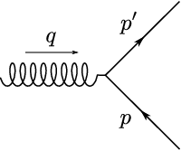
Refer to caption
(a) Tree Level
Refer to caption
(b) Self Energy
Refer to caption
(c) Counter Term
Refer to caption
(d) Electromagnetic Vertex
Refer to caption
(e) Contact
Refer to caption
(f) Photon Polarization
Figure 2: The diagrams contributing to the radiative corrections to the stress-energy tensor. The curly line is the stress-energy tensor, the wavy line is the photon and the solid line is the fermion.

In order to evaluate the radiative corrections to gravitomagnetic moment at finite temperature we have to consider the renormalization of the stress-energy tensor at finite temperature and at first order on momentum transfer qq. The zero temperature renormalization is performed with usual techniques and we do not discuss it here. To address thermal corrections to the matrix-element of stress-energy tensor we use the real-time formalism of thermal field theory. The major modification of QFT at finite temperature is the value of the vacuum of the theory, which is not empty but contain a number of bosons and fermions given respectively by the Bose-Einstein and the Fermi-Dirac distribution functions:

a^B†​a^B​(p)​|0⟩=nB​(E)​|0⟩,a^F†​a^F​(p)​|0⟩=nF​(E)​|0⟩,\widehat{a}_{\textup{B}}^{\dagger}\widehat{a}_{\textup{B}}(p)|0\rangle=n_{\textup{B}}(E)|0\rangle,\quad\widehat{a}_{\textup{F}}^{\dagger}\widehat{a}_{\textup{F}}(p)|0\rangle=n_{\textup{F}}(E)|0\rangle,

where as usual we indicate

nB​(x)=1exp⁡(β​x)−1,nF​(x)=1exp⁡(β​x)+1.n_{\textup{B}}(x)=\frac{1}{\exp(\beta x)-1},\quad n_{\textup{F}}(x)=\frac{1}{\exp(\beta x)+1}.

The resulting propagators of the gauge field and of the fermionic field in real-time formalism are

i​SF​(p)=(p̸+m)​[ip2−m2−2​π​δ​(p2−m2)​nF​(p)],i​Dμ​ν​(k)=−ημ​ν​[ik2+2​π​δ​(k2)​nB​(k)].\begin{split}\mathrm{i}S_{F}(p)&=\left(\not{p}+m\right)\left[\frac{\mathrm{i}}{p^{2}-m^{2}}-2\pi\delta\left(p^{2}-m^{2}\right)n_{F}(p)\right],\\ \mathrm{i}D_{\mu\nu}(k)&=-\eta_{\mu\nu}\left[\frac{\mathrm{i}}{k^{2}}+2\pi\delta\left(k^{2}\right)n_{B}(k)\right].\end{split}

Perturbation theory and Feynman diagrams at finite temperature are unmodified compared to usual quantum field theory except for the previous propagators. We see that the propagators in real-time formalism are naturally separated into a temperature part and into a T=0T=0 part. The T=0T=0 part has been addressed as usual and from now on we just consider the thermal part. The diagrams responsible for radiative corrections to the stress-energy tensor matrix element

⟨p′,s′​|Tμ​ν​(0)|​p,s⟩=1Z2​(p)​Z2​(p′)​u¯β​(p′)​Mμ​ν​(p,p′)​uβ​(p),\langle p^{\prime},s^{\prime}|T^{\mu\nu}(0)|p,s\rangle=\frac{1}{\sqrt{Z_{2}(p)Z_{2}(p^{\prime})}}\bar{u}_{\beta}(p^{\prime})M_{\mu\nu}(p,p^{\prime})u_{\beta}(p),

are reported in Fig. 2. Furthermore, since we are only interested in the thermal part, each integrals corresponding to a Feynman diagram is weighted with a thermal function and it is therefore ultraviolet convergent and finite. All the divergent part are already been taken care of with the T=0T=0 renormalization.

Note that we can distinguish between two different regimes of temperature. Indeed, finite-temperature modification may arise both from the boson or the photon propagators. However, for low temperatures such that T≪mT\ll m, the fermion distribution function is suppressed by a factor exp(−m/T)\exp(-m/T), which is negligible compared to contributions of order (T/m)2(T/m)^{2} coming from the photon distribution. In the opposite regime, when T≫mT\gg m, the photon contribution is still the same as low temperatures, while the fermion distribution can now also contribute with terms of order (T/m)2(T/m)^{2}. Therefore, as in the case of the pole of the propagator, we can expect two different values of AGM valid in the two regimes of low and high temperatures.

As first step, we need to identify the mass shift and the wave-function renormalization constant. These quantities are obtained starting from the self-energy of the fermion, which is discussed in Sec. A.1. We found that the self-energy can be written as Σ⁡(p)=a​p̸+b​u̸+c\Sigma(p)=a\not{p}+b\not{u}+c and that the full fermion propagator becomes

S⁡(p)=(1−a)​p̸−b​u̸+m+c[(1−a)​p−b​u]2−(m+c)2,S(p)=\frac{(1-a)\not{p}-b\not{u}+m+c}{[(1-a)p-bu]^{2}-(m+c)^{2}}, (30)

which has a pole in ω2=Eβ2=ps2+mp2\omega^{2}=E_{\beta}^{2}=p_{s}^{2}+m_{p}^{2}, with mpm_{p} given by Eq. (27).

C.1 Thermal Dirac spinor

The Dirac equation in momentum space is modified according to the self-energy, which also include thermal modifications. The thermal Dirac spinors uβ​(p)u_{\beta}(p) satisfy the modified Dirac equation corresponding to the new propagator (30):

[p̸−mR−Σβ​(p)]​uβ​(p)=[(1−a)​p̸−b​u̸−mR−c]​uβ​(p)=0,\left[\not{p}-m_{R}-\Sigma^{\beta}(p)\right]u_{\beta}(p)=\left[(1-a)\not{p}-b\not{u}-m_{R}-c\right]u_{\beta}(p)=0,

where mRm_{R} indicates the zero temperature renormalized mass. The thermal spinor uβ​(p)u_{\beta}(p) satisfies the previous equation when pp is the pole of the propagator, i.e. such that p⋅u=Eβ​(ps)p\cdot u=E_{\beta}(p_{s}). The thermal Dirac spinors are actually required to properly account for stress-energy tensor renormalization at finite temperature Donoghue et al. 1984; Weldon 1982b.

In thermal bath rest frame, we choose the normalization

uβ†​(p)​uβ​(p)=1.u^{\dagger}_{\beta}(p)u_{\beta}(p)=1.

For convenience, we furthermore define a four vector and a scalar

pT≡(1−a)​p−b​u,mT≡mR+c,p_{T}\equiv(1-a)p-bu,\quad m_{T}\equiv m_{R}+c,

so that the modified thermal Dirac equation is written as

[p̸T−mT]​uβ​(p)=0.\left[\not{p}_{T}-m_{T}\right]u_{\beta}(p)=0.

Therefore, it follows from the modified thermal Dirac equation that the thermal spinors satisfy the following identities:

u¯β​(p,s)​uβ​(p,s)=mT(1−a)​Eβ−b,u¯β​(p,s)​γμ​uβ​(p,s)=pTμ(1−a)​Eβ−b,∑suβ​(p,s)​u¯β​(p,s)=p̸T+mT2​(1−a)​Eβ−2​b.\bar{u}_{\beta}(p,s)u_{\beta}(p,s)=\frac{m_{T}}{(1-a)E_{\beta}-b},\quad\bar{u}_{\beta}(p,s)\gamma_{\mu}u_{\beta}(p,s)=\frac{{p_{T}}_{\mu}}{(1-a)E_{\beta}-b},\quad\sum_{s}u_{\beta}(p,s)\bar{u}_{\beta}(p,s)=\frac{\not{p}_{T}+m_{T}}{2(1-a)E_{\beta}-2b}.

In the non relativistic limit and in the frame where u=(1,𝟎)u=(1,\mathchoice{\mbox{\boldmath$\displaystyle\mathbf{0}$}}{\mbox{\boldmath$\textstyle\mathbf{0}$}}{\mbox{\boldmath$\scriptstyle\mathbf{0}$}}{\mbox{\boldmath$\scriptscriptstyle\mathbf{0}$}}), we can also show the validity of the following identities:

u¯β​(p′)​γ0​uβ​(p)=ξ′⁣†​ξ+𝒪⁡(e2),u¯β​(p′)​𝜸​uβ​(p)=ξ′⁣†​[𝐏2​mp+i​𝝈∧𝐪2​mp]​ξ+𝒪⁡(e4),\bar{u}_{\beta}(p^{\prime})\gamma_{0}u_{\beta}(p)=\xi^{\prime\dagger}\xi+\mathcal{O}(e^{2}),\quad\bar{u}_{\beta}(p^{\prime})\mathchoice{\mbox{\boldmath$\displaystyle\mathbf{\gamma}$}}{\mbox{\boldmath$\textstyle\mathbf{\gamma}$}}{\mbox{\boldmath$\scriptstyle\mathbf{\gamma}$}}{\mbox{\boldmath$\scriptscriptstyle\mathbf{\gamma}$}}u_{\beta}(p)=\xi^{\prime\dagger}\left[\frac{\mathchoice{\mbox{\boldmath$\displaystyle\mathbf{P}$}}{\mbox{\boldmath$\textstyle\mathbf{P}$}}{\mbox{\boldmath$\scriptstyle\mathbf{P}$}}{\mbox{\boldmath$\scriptscriptstyle\mathbf{P}$}}}{2m_{p}}+\mathrm{i}\frac{\mathchoice{\mbox{\boldmath$\displaystyle\mathbf{\sigma}$}}{\mbox{\boldmath$\textstyle\mathbf{\sigma}$}}{\mbox{\boldmath$\scriptstyle\mathbf{\sigma}$}}{\mbox{\boldmath$\scriptscriptstyle\mathbf{\sigma}$}}\wedge\mathchoice{\mbox{\boldmath$\displaystyle\mathbf{q}$}}{\mbox{\boldmath$\textstyle\mathbf{q}$}}{\mbox{\boldmath$\scriptstyle\mathbf{q}$}}{\mbox{\boldmath$\scriptscriptstyle\mathbf{q}$}}}{2m_{p}}\right]\xi+\mathcal{O}(e^{4}),

where ξ\xi is the two component spinor, normalized such that ξ†​ξ=1\xi^{\dagger}\xi=1. We used the identities above to compute the gravitational mass in Sec. A.3 and the gravitomagnetic moment in Sec. IV.

C.2 Wave-function renormalization constant Z2Z_{2}

The wave-function renormalization constant Z2Z_{2} is obtained by requesting that the fermion field is properly renormalized

ψR​(x)=1Z2​ψ0​(x).\psi_{\textup{R}}(x)=\frac{1}{\sqrt{Z_{2}}}\psi_{0}(x).

The temperature part of the wave-function renormalization constant is Donoghue and Holstein 1983; Mitra et al. 2001

Z2β​(ω,ps)=2​[(1−a)​Eβ−b]∂D∂ω|ω=Eβ,{}^{\beta}Z_{2}(\omega,p_{s})=\frac{2\left[(1-a)E_{\beta}-b\right]}{\frac{\partial D}{\partial\omega}\Big|_{\omega=E_{\beta}}},

where EβE_{\beta} is the pole of the propagator and DD is the denominator of the propagator (30)

D⁡(ω,ps)=(1−a)2​(ω2−ps2)+b2−2​(1−a)​b​ω−(m+c)2.D(\omega,p_{s})=(1-a)^{2}(\omega^{2}-p_{s}^{2})+b^{2}-2(1-a)b\omega-(m+c)^{2}.

At order e2e^{2} we find

βZ2=1+(a+m2ω∂a∂ω+∂b∂ω+mω∂c∂ω)|ω=ps2+m2.^{\beta}Z_{2}=1+\left(a+\frac{m^{2}}{\omega}\frac{\partial a}{\partial\omega}+\frac{\partial b}{\partial\omega}+\frac{m}{\omega}\frac{\partial c}{\partial\omega}\right)\Big|_{\omega=\sqrt{p_{s}^{2}+m^{2}}}. (31)

For the computation of AGM we are interested to the quantity (Z2​(p)​Z2​(p′))−1/2(\sqrt{Z_{2}(p)Z_{2}(p^{\prime})})^{-1/2} in the limits of q→0q\to 0 and of Ps=(P⋅u)2−P2→0P_{s}=\sqrt{(P\cdot u)^{2}-P^{2}}\to 0. Therefore, we just have to evaluate Z2​(p)Z_{2}(p) with pp an on-shell momentum and then perform the ps→0p_{s}\to 0 limit. Using the prescription in Eq. (31) and the behavior of the functions a,b,ca,b,c we find:

limps→0βZ2​(p)=1−e2​T212​m2+e22​π2​∫0∞d​k​nB​(k)k−θHT​e2​T224​m2,\lim_{p_{s}\to 0}\,^{\beta}Z_{2}(p)=1-\frac{e^{2}T^{2}}{12m^{2}}+\frac{e^{2}}{2\pi^{2}}\int_{0}^{\infty}{\rm d}k\,\frac{n_{\textup{B}}(k)}{k}-\theta_{\textup{HT}}\frac{e^{2}T^{2}}{24m^{2}},

where the θHT\theta_{\textup{HT}} is defined such that it turns on the high temperatures contribution:

θHT≡{0T≪m1T≫m.\theta_{\textup{HT}}\equiv\begin{cases}0&T\ll m\\ 1&T\gg m\end{cases}.

The low-temperature part is in agreement with Donoghue and Holstein 1983; Donoghue et al. 1984; Mitra et al. 2001. Therefore we have

limps→01Z2β​(p)β​Z2​(p′)=1+e2​T212​m2−e216​π3​IA+θHT​e2​T224​m2,\lim_{p_{s}\to 0}\frac{1}{\sqrt{\,{}^{\beta}Z_{2}(p)\,^{\beta}Z_{2}(p^{\prime})}}=1+\frac{e^{2}T^{2}}{12m^{2}}-\frac{e^{2}}{16\pi^{3}}I_{\textup{A}}+\theta_{\textup{HT}}\,\frac{e^{2}T^{2}}{24m^{2}},

where we denoted

IA≡8​π​∫0∞d​k​nB​(k)k.I_{\textup{A}}\equiv 8\pi\int_{0}^{\infty}{\rm d}k\,\frac{n_{\textup{B}}(k)}{k}.

For future convenience, noticing that for ps=0p_{s}=0 we have ωP=2​m\omega_{P}=2m, we can write the factor coming from wave-function renormalization constants using ωP≡u⋅P\omega_{P}\equiv u\cdot P instead of the mass mm:

limPs→0limq→01Z2β​(p)β​Z2​(p′)=1+e2​T23​ωP2−e216​π3​IA+θHT​e2​T26​ωP2.\lim_{P_{s}\to 0}\lim_{q\to 0}\frac{1}{\sqrt{\,{}^{\beta}Z_{2}(p)\,^{\beta}Z_{2}(p^{\prime})}}=1+\frac{e^{2}T^{2}}{3\omega_{P}^{2}}-\frac{e^{2}}{16\pi^{3}}I_{\textup{A}}+\theta_{\textup{HT}}\,\frac{e^{2}T^{2}}{6\omega_{P}^{2}}.

C.3 Renormalization of stress-energy tensor at finite temperature

As last step to renormalize the stress-energy tensor we have to calculate the temperature contribution of the diagrams in Fig. 2. Here we write the general procedure and we leave the details in Appendix D.

First, we recap the notation used. We indicate with qq and PP the momenta

P=p′+p,q=p′−pP=p^{\prime}+p,\quad q=p^{\prime}-p

where pp and p′p^{\prime} are the momenta of external legs of the diagrams in Fig. 2. Notice that q⋅P=0q\cdot P=0. Moreover, scattering theory imposes the conservation of the time component of pp and p′p^{\prime} in the thermal bath rest frame, meaning q⋅u=0q\cdot u=0. We are using this constraint when evaluating all the diagrams. It is then convenient to define the following scalar and four-vectors:

ωP=P⋅u,Ps=ωP2−P2,P~μ=(ημ​ν−uμ​uν)​Pν=Pμ−ωP​uμ,lμ=ϵμ​ν​ρ​σ​uν​P~ρ​qσ,l^μ=lμ−l2,\omega_{P}=P\cdot u,\quad P_{s}=\sqrt{\omega_{P}^{2}-P^{2}},\quad\tilde{P}_{\mu}=(\eta_{\mu\nu}-u_{\mu}u_{\nu})P^{\nu}=P_{\mu}-\omega_{P}u_{\mu},\quad l^{\mu}=\epsilon^{\mu\nu\rho\sigma}u_{\nu}\tilde{P}_{\rho}q_{\sigma},\quad\hat{l}^{\mu}=\frac{l^{\mu}}{\sqrt{-l^{2}}},

we also denote with aa the ratio

a≡ωP2−P2ωP=PsωP,0<a<1.a\equiv\frac{\sqrt{\omega_{P}^{2}-P^{2}}}{\omega_{P}}=\frac{P_{s}}{\omega_{P}},\quad 0<a<1.

Since we are considering 1-loop corrections, a generic diagrams of Fig. 2, which we label with XX, can be written as

Mμ​νX​(p,p′)=∫d4​k(2​π)4​fX​(p,p′,k)DX​(p,p′,k)​u¯​(p′)​Nμ​νX​u​(p),M_{\mu\nu}^{X}(p,p^{\prime})=\int\frac{{\rm d}^{4}k}{(2\pi)^{4}}\frac{f^{X}(p,p^{\prime},k)}{D^{X}(p,p^{\prime},k)}\bar{u}(p^{\prime})N^{X}_{\mu\nu}u(p), (32)

where all the spinorial structure is contained inside the numerator NXN^{X}. Therefore NXN^{X} can be simplified using Dirac equation and it can be decomposed in the following terms:

u¯​(p′)​Nμ​νX​u​(p)=u¯(p′)[Nk​kXk̸kμkν+NP​kXk̸(Pμkν+Pνkμ)++(NP​γX⁡(s)+NP​γX⁡(k)k̸)(Pμγν+Pνγμ)+(Nk​γX⁡(s)+Nk​γX⁡(k)k̸)(kμγν+kνγμ)+⋯]u(p)\begin{split}\bar{u}(p^{\prime})N^{X}_{\mu\nu}u(p)=&\bar{u}(p^{\prime})\Big[N_{kk}^{X}\not{k}\,k_{\mu}k_{\nu}+N_{Pk}^{X}\not{k}\,(P_{\mu}k_{\nu}+P_{\nu}k_{\mu})+\\ &+(N_{P\gamma}^{X(s)}+N_{P\gamma}^{X(k)}\not{k})(P_{\mu}\gamma_{\nu}+P_{\nu}\gamma_{\mu})+(N_{k\gamma}^{X(s)}+N_{k\gamma}^{X(k)}\not{k})(k_{\mu}\gamma_{\nu}+k_{\nu}\gamma_{\mu})+\cdots\Big]u(p)\end{split} (33)

where each term Ny​yXN_{yy}^{X} can depend on the scalars {k2,P2,q2,k⋅P,k⋅q,P⋅q,m}\{k^{2},\,P^{2},\,q^{2},k\cdot P,\,k\cdot q,\,P\cdot q,\,m\} and the dots stands for terms that to do not contribute to AGM. Indeed, we show in App. B that the only terms that are relevant for AGM are

uμ​γν+uν​γμ,Pμ​γν+Pν​γμ,l^​(uμ​l^ν+uν​l^μ),l^​(Pμ​l^ν+Pν​l^μ).\begin{split}u_{\mu}\gamma_{\nu}+u_{\nu}\gamma_{\mu},&\quad P_{\mu}\gamma_{\nu}+P_{\nu}\gamma_{\mu},\quad\not{\hat{l}}\left(u_{\mu}\hat{l}_{\nu}+u_{\nu}\hat{l}_{\mu}\right),\quad\not{\hat{l}}\left(P_{\mu}\hat{l}_{\nu}+P_{\nu}\hat{l}_{\mu}\right).\end{split}

Using the orthogonal non-normalized basis {u,P~,q,l^}\{u,\,\tilde{P},\,q,\,\hat{l}\}, the integration variable kk can be decomposed into:

kμ=(k⋅u)​uμ+(k⋅P~)P~2​P~μ+(k⋅q)q2​qμ−(k⋅l^)​l^μ=[(k⋅u)−ωP​(k⋅P~)P~2]​uμ+(k⋅P~)P~2​Pμ+(k⋅q)q2​qμ−(k⋅l^)​l^μ≡Au​uμ+AP​Pμ+Aq​qμ+Al​l^μ.\begin{split}k_{\mu}=&(k\cdot u)u_{\mu}+\frac{(k\cdot\tilde{P})}{\tilde{P}^{2}}\tilde{P}_{\mu}+\frac{(k\cdot q)}{q^{2}}q_{\mu}-(k\cdot\hat{l})\hat{l}_{\mu}\\ =&\left[(k\cdot u)-\frac{\omega_{P}(k\cdot\tilde{P})}{\tilde{P}^{2}}\right]u_{\mu}+\frac{(k\cdot\tilde{P})}{\tilde{P}^{2}}P_{\mu}+\frac{(k\cdot q)}{q^{2}}q_{\mu}-(k\cdot\hat{l})\hat{l}_{\mu}\\ \equiv&A_{u}\,u_{\mu}+A_{P}\,P_{\mu}+A_{q}\,q_{\mu}+A_{l}\,\hat{l}_{\mu}.\end{split}

This decomposition is used to write the diagrams in a covariant form. Consider the term u¯​(p′)​k̸​u​(p)​vμ​wμ\bar{u}(p^{\prime})\not{k}u(p)v_{\mu}w_{\mu}, where vv and ww are any vector between {u,P,q,l}\{u,P,q,l\}, the term is decomposed into

u¯​(p′)​k̸​u​(p)​vμ​wν=u¯​(p′)​[Au​u̸+Al​l^+2​m​AP]​u​(p)​vμ​wν,\bar{u}(p^{\prime})\not{k}u(p)v_{\mu}w_{\nu}=\bar{u}(p^{\prime})\left[A_{u}\,\not{u}+A_{l}\,\not{\hat{l}}+2mA_{P}\right]u(p)v_{\mu}w_{\nu},

and for what we show in Sec. IV.2 only the term in l̸\not{l} can contribute to AGM:

u¯​(p′)​k̸​u​(p)​vμ​wν→Al​u¯​(p′)​l^​vμ​wν​u​(p) with ​(v,w)=(u,l)​ or ​(v,w)=(P,l).\bar{u}(p^{\prime})\not{k}u(p)v_{\mu}w_{\nu}\to A_{l}\,\bar{u}(p^{\prime})\,\not{\hat{l}}\,v_{\mu}w_{\nu}\,u(p)\quad\text{ with }(v,w)=(u,l)\text{ or }(v,w)=(P,l).

With the same argument, we can select only the parts relevant to AGM of all the possible terms:

u¯​(p′)​k̸​u​(p)​(kμ​vν+kν​vμ)→u¯​(p′)​[Au​Al​l^​(uμ​vν+uν​vμ)+AP​Al​l^​(Pμ​vν+Pν​vμ)]​u​(p)​ if ​v=l→u¯​(p′)​[Al2​l^​(l^μ​vν+l^ν​vμ)]​u​(p)​ if ​v=u​ or ​v=Pu¯​(p′)​k̸​kμ​kν​u​(p)→u¯​(p′)​[Au​Al2​l^​(uμ​l^ν+uν​l^μ)+AP​Al2​l^​(Pμ​l^ν+Pν​l^μ)]​u​(p).\begin{split}\bar{u}(p^{\prime})\not{k}u(p)\left(k_{\mu}v_{\nu}+k_{\nu}v_{\mu}\right)\to&\bar{u}(p^{\prime})\Big[A_{u}A_{l}\not{\hat{l}}(u_{\mu}v_{\nu}+u_{\nu}v_{\mu})+A_{P}A_{l}\not{\hat{l}}(P_{\mu}v_{\nu}+P_{\nu}v_{\mu})\Big]u(p)\text{ if }v=l\\ \to&\bar{u}(p^{\prime})\Big[A_{l}^{2}\not{\hat{l}}(\hat{l}_{\mu}v_{\nu}+\hat{l}_{\nu}v_{\mu})\Big]u(p)\text{ if }v=u\text{ or }v=P\\ \bar{u}(p^{\prime})\not{k}k_{\mu}k_{\nu}u(p)\to&\bar{u}(p^{\prime})\Big[A_{u}A_{l}^{2}\,\not{\hat{l}}(u_{\mu}\hat{l}_{\nu}+u_{\nu}\hat{l}_{\mu})+A_{P}A_{l}^{2}\,\not{\hat{l}}(P_{\mu}\hat{l}_{\nu}+P_{\nu}\hat{l}_{\mu})\Big]u(p).\end{split}

We then approximate the integrand to first order in qq and we perform the loop integral in kk decomposing its component along the tetrad {u,P~,q,l}\{u,\tilde{P},q,l\}. The results at first order in qq are (see Appendix D):

(Z2(p)Z2(p′))−1/2Mμ​ν(0)=IP​γZ​(Pμ​γν+Pν​γμ),Mμ​νS​E+Mμ​νC​T=IP​γS​(Pμ​γν+Pν​γμ),Mμ​νV=(IP​γV+θHT​IP​γ,fV)​(Pμ​γν+Pν​γμ)+(Iu​γV+θHT​Iu​γ,fV)​(uμ​γν+uν​γμ)+(IP​lV+θHT​IP​l,fV)​l^​(Pμ​l^ν+Pν​l^μ)+θHT​Iu​l,fV​l^​(uμ​l^ν+uν​l^μ),Mμ​νC=(IP​γC+θHT​IP​γ,fC)​(Pμ​γν+Pν​γμ)+(Iu​γC+θHT​Iu​γ,fC)​(uμ​γν+uν​γμ),Mμ​νP=IP​γP​(Pμ​γν+Pν​γμ)+Iu​γP​(uμ​γν+uν​γμ)+(IP​lP+θHT​IP​l,fP)​l^​(Pμ​l^ν+Pν​l^μ)+(Iu​lP+θHT​Iu​l,fP)​l^​(uμ​l^ν+uν​l^μ).\begin{split}(Z_{2}(p)Z_{2}(p^{\prime}))^{-1/2}M_{\mu\nu}^{(0)}=&I^{Z}_{P\gamma}\left(P_{\mu}\gamma_{\nu}+P_{\nu}\gamma_{\mu}\right),\\ M_{\mu\nu}^{SE}+M_{\mu\nu}^{CT}=&I^{S}_{P\gamma}\left(P_{\mu}\gamma_{\nu}+P_{\nu}\gamma_{\mu}\right),\\ M_{\mu\nu}^{V}=&\left(I^{V}_{P\gamma}+\theta_{\textup{HT}}I^{V}_{P\gamma,f}\right)\left(P_{\mu}\gamma_{\nu}+P_{\nu}\gamma_{\mu}\right)+\left(I^{V}_{u\gamma}+\theta_{\textup{HT}}I^{V}_{u\gamma,f}\right)\left(u_{\mu}\gamma_{\nu}+u_{\nu}\gamma_{\mu}\right)\\ &+\left(I^{V}_{Pl}+\theta_{\textup{HT}}I^{V}_{Pl,f}\right)\not{\hat{l}}\left(P_{\mu}\hat{l}_{\nu}+P_{\nu}\hat{l}_{\mu}\right)+\theta_{\textup{HT}}I^{V}_{ul,f}\not{\hat{l}}\left(u_{\mu}\hat{l}_{\nu}+u_{\nu}\hat{l}_{\mu}\right),\\ M_{\mu\nu}^{C}=&\left(I^{C}_{P\gamma}+\theta_{\textup{HT}}I^{C}_{P\gamma,f}\right)\left(P_{\mu}\gamma_{\nu}+P_{\nu}\gamma_{\mu}\right)+\left(I^{C}_{u\gamma}+\theta_{\textup{HT}}I^{C}_{u\gamma,f}\right)\left(u_{\mu}\gamma_{\nu}+u_{\nu}\gamma_{\mu}\right),\\ M_{\mu\nu}^{P}=&I^{P}_{P\gamma}\left(P_{\mu}\gamma_{\nu}+P_{\nu}\gamma_{\mu}\right)+I^{P}_{u\gamma}\left(u_{\mu}\gamma_{\nu}+u_{\nu}\gamma_{\mu}\right)+\left(I^{P}_{Pl}+\theta_{\textup{HT}}I^{P}_{Pl,f}\right)\not{\hat{l}}\left(P_{\mu}\hat{l}_{\nu}+P_{\nu}\hat{l}_{\mu}\right)\\ &+\left(I^{P}_{ul}+\theta_{\textup{HT}}I^{P}_{ul,f}\right)\not{\hat{l}}\left(u_{\mu}\hat{l}_{\nu}+u_{\nu}\hat{l}_{\mu}\right).\end{split}

Here, the function

θHT≡{0T≪m1T≫m\theta_{\textup{HT}}\equiv\begin{cases}0&T\ll m\\ 1&T\gg m\end{cases}

turns on the fermionic contributions at high temperature and removes them for low temperatures; we also introduce the IR divergent integral

IA≡8​π​∫0∞d​k​nB​(k)k.I_{\textup{A}}\equiv 8\pi\int_{0}^{\infty}{\rm d}k\frac{n_{\textup{B}}(k)}{k}.

The form factors of Pμ​γν+Pν​γμP_{\mu}\gamma_{\nu}+P_{\nu}\gamma_{\mu} are

limPs→0limq→0IP​γZ=14+2+θHT24​e2​T2ωP2−14​e216​π3​IA;limPs→0limq→0IP​γS=−2+θHT12​e2​T2ωP2+12​e216​π3​IA;IP​γV=−118​e2​T2ωP2​[32​a3​log⁡(1+a1−a)−3a2]−14​e216​π3​4​m2ωP2​IA1−a2;IP​γ,fV=−136​e2​T2ωP2​[32​a3​log⁡(1+a1−a)−3a2];IP​γC=118​e2​T2ωP2​[32​a3​log⁡(1+a1−a)−3a2];IP​γ,fC=136​e2​T2ωP2​[32​a3​log⁡(1+a1−a)−3a2];IP​γP=−118​e2​T2ωP2​[32​a3​log⁡(1+a1−a)−3a2].\begin{split}\lim_{P_{s}\to 0}\lim_{q\to 0}I^{Z}_{P\gamma}=&\frac{1}{4}+\frac{2+\theta_{\textup{HT}}}{24}\frac{e^{2}T^{2}}{\omega_{P}^{2}}-\frac{1}{4}\frac{e^{2}}{16\pi^{3}}I_{\textup{A}};\\ \lim_{P_{s}\to 0}\lim_{q\to 0}I^{S}_{P\gamma}=&-\frac{2+\theta_{\textup{HT}}}{12}\frac{e^{2}T^{2}}{\omega_{P}^{2}}+\frac{1}{2}\frac{e^{2}}{16\pi^{3}}I_{\textup{A}};\\ I^{V}_{P\gamma}=&-\frac{1}{18}\frac{e^{2}T^{2}}{\omega_{P}^{2}}\left[\frac{3}{2a^{3}}\log\left(\frac{1+a}{1-a}\right)-\frac{3}{a^{2}}\right]-\frac{1}{4}\frac{e^{2}}{16\pi^{3}}\frac{4m^{2}}{\omega_{P}^{2}}\frac{I_{A}}{1-a^{2}};\\ I^{V}_{P\gamma,f}=&-\frac{1}{36}\frac{e^{2}T^{2}}{\omega_{P}^{2}}\left[\frac{3}{2a^{3}}\log\left(\frac{1+a}{1-a}\right)-\frac{3}{a^{2}}\right];\\ I^{C}_{P\gamma}=&\frac{1}{18}\frac{e^{2}T^{2}}{\omega_{P}^{2}}\left[\frac{3}{2a^{3}}\log\left(\frac{1+a}{1-a}\right)-\frac{3}{a^{2}}\right];\\ I^{C}_{P\gamma,f}=&\frac{1}{36}\frac{e^{2}T^{2}}{\omega_{P}^{2}}\left[\frac{3}{2a^{3}}\log\left(\frac{1+a}{1-a}\right)-\frac{3}{a^{2}}\right];\\ I^{P}_{P\gamma}=&-\frac{1}{18}\frac{e^{2}T^{2}}{\omega_{P}^{2}}\left[\frac{3}{2a^{3}}\log\left(\frac{1+a}{1-a}\right)-\frac{3}{a^{2}}\right].\end{split}

The form factors of uμ​γν+uν​γμu_{\mu}\gamma_{\nu}+u_{\nu}\gamma_{\mu} are

Iu​γV=−19​e2​T2ωP​[32​a3​log⁡(1+a1−a)−3a2];Iu​γ,fV=−118​e2​T2ωP​[32​a2−3​(1−a2)4​a3​log⁡(1+a1−a)];Iu​γC=19​e2​T2ωP​[32​a2−3​(1−a2)4​a3​log⁡(1+a1−a)];Iu​γ,fC=118​e2​T2ωP​[32​a2−3​(1−a2)4​a3​log⁡(1+a1−a)];Iu​γP=−19​e2​T2ωP​[32​a2−3​(1−a2)4​a3​log⁡(1+a1−a)].\begin{split}I^{V}_{u\gamma}=&-\frac{1}{9}\frac{e^{2}T^{2}}{\omega_{P}}\left[\frac{3}{2a^{3}}\log\left(\frac{1+a}{1-a}\right)-\frac{3}{a^{2}}\right];\\ I^{V}_{u\gamma,f}=&-\frac{1}{18}\frac{e^{2}T^{2}}{\omega_{P}}\left[\frac{3}{2a^{2}}-\frac{3(1-a^{2})}{4a^{3}}\log\left(\frac{1+a}{1-a}\right)\right];\\ I^{C}_{u\gamma}=&\frac{1}{9}\frac{e^{2}T^{2}}{\omega_{P}}\left[\frac{3}{2a^{2}}-\frac{3(1-a^{2})}{4a^{3}}\log\left(\frac{1+a}{1-a}\right)\right];\\ I^{C}_{u\gamma,f}=&\frac{1}{18}\frac{e^{2}T^{2}}{\omega_{P}}\left[\frac{3}{2a^{2}}-\frac{3(1-a^{2})}{4a^{3}}\log\left(\frac{1+a}{1-a}\right)\right];\\ I^{P}_{u\gamma}=&-\frac{1}{9}\frac{e^{2}T^{2}}{\omega_{P}}\left[\frac{3}{2a^{2}}-\frac{3(1-a^{2})}{4a^{3}}\log\left(\frac{1+a}{1-a}\right)\right].\end{split}

The form factors of l^​(Pμ​l^ν+Pν​l^μ)\not{\hat{l}}(P_{\mu}\hat{l}_{\nu}+P_{\nu}\hat{l}_{\mu}) are

IP​lV=112​e2​T2ωP2​[32​a3​log⁡(1+a1−a)−3a2];IP​l,fV=7360​e2​T2ωP2​[127​4​m2ωP2​(5​(3−2​a2)2​a4​(1−a2)−154​a5​log⁡(1+a1−a))−57​(32​a3​log⁡(1+a1−a)−3a2)];IP​lP=IP​γP=−118​e2​T2ωP2​[32​a3​log⁡(1+a1−a)−3a2];IP​l,fP=−130​e2​T2ωP2​4​m2ωP2​[15​(3−a2)8​a5​log⁡(1+a1−a)−454​a4].\begin{split}I^{V}_{Pl}=&\frac{1}{12}\frac{e^{2}T^{2}}{\omega_{P}^{2}}\left[\frac{3}{2a^{3}}\log\left(\frac{1+a}{1-a}\right)-\frac{3}{a^{2}}\right];\\ I^{V}_{Pl,f}=&\frac{7}{360}\frac{e^{2}T^{2}}{\omega_{P}^{2}}\left[\frac{12}{7}\frac{4m^{2}}{\omega_{P}^{2}}\left(\frac{5(3-2a^{2})}{2a^{4}(1-a^{2})}-\frac{15}{4a^{5}}\log\left(\frac{1+a}{1-a}\right)\right)-\frac{5}{7}\left(\frac{3}{2a^{3}}\log\left(\frac{1+a}{1-a}\right)-\frac{3}{a^{2}}\right)\right];\\ I^{P}_{Pl}=&I^{P}_{P\gamma}=-\frac{1}{18}\frac{e^{2}T^{2}}{\omega_{P}^{2}}\left[\frac{3}{2a^{3}}\log\left(\frac{1+a}{1-a}\right)-\frac{3}{a^{2}}\right];\\ I^{P}_{Pl,f}=&-\frac{1}{30}\frac{e^{2}T^{2}}{\omega_{P}^{2}}\frac{4m^{2}}{\omega_{P}^{2}}\left[\frac{15(3-a^{2})}{8a^{5}}\log\left(\frac{1+a}{1-a}\right)-\frac{45}{4a^{4}}\right].\end{split}

The form factors of l^​(uμ​l^ν+uν​l^μ)\not{\hat{l}}(u_{\mu}\hat{l}_{\nu}+u_{\nu}\hat{l}_{\mu}) are

Iu​l,fV=−130​e2​T2ωP​[−23​4​m2ωP2​(15​(3−2​a2)8​a5​log⁡(1+a1−a)−454​a4)+53​(32​a2−3​(1−a2)4​a3​log⁡(1+a1−a))];Iu​lP=Iu​γP=−19​e2​T2ωP​[32​a2−3​(1−a2)4​a3​log⁡(1+a1−a)];Iu​l,fP=−145​e2​T2ωP​4​m2ωP2​[15​(3−a2)8​a5​log⁡(1+a1−a)−454​a4].\begin{split}I^{V}_{ul,f}=&-\frac{1}{30}\frac{e^{2}T^{2}}{\omega_{P}}\left[-\frac{2}{3}\frac{4m^{2}}{\omega_{P}^{2}}\left(\frac{15(3-2a^{2})}{8a^{5}}\log\left(\frac{1+a}{1-a}\right)-\frac{45}{4a^{4}}\right)+\frac{5}{3}\left(\frac{3}{2a^{2}}-\frac{3(1-a^{2})}{4a^{3}}\log\left(\frac{1+a}{1-a}\right)\right)\right];\\ I^{P}_{ul}=&I^{P}_{u\gamma}=-\frac{1}{9}\frac{e^{2}T^{2}}{\omega_{P}}\left[\frac{3}{2a^{2}}-\frac{3(1-a^{2})}{4a^{3}}\log\left(\frac{1+a}{1-a}\right)\right];\\ I^{P}_{ul,f}=&-\frac{1}{45}\frac{e^{2}T^{2}}{\omega_{P}}\frac{4m^{2}}{\omega_{P}^{2}}\left[\frac{15(3-a^{2})}{8a^{5}}\log\left(\frac{1+a}{1-a}\right)-\frac{45}{4a^{4}}\right].\end{split}

These functions are written such that the quantity inside the square brackets is 1 for a=0a=0, which correspond to the non relativistic particle limit (Ps→0P_{s}\to 0). It is straightforward to check that by summing all these terms in the non-relativistic limit, one get the form factors quoted in Eq. (21).

Appendix D Radiative correction to the stress-energy tensor

In this appendix we evaluate the temperature modification of the diagrams in Fig. 2. The general strategy and the final results are written in Sec. C.3, in what follows we provide a detailed calculations of all the diagrams.

To perform the loop integration on the momentum kk in the generic diagram (32), since the set {u,P~,q,l^}\{u,\,\tilde{P},\,q,\,\hat{l}\} is a basis, we choose k0k_{0} along uu, kzk_{z} along qμq_{\mu} and kxk_{x} along P~\tilde{P} and kyk_{y} along ll; thus, defining

ϵ=−q2,a=−P~2ωP=ωP2−P2ωP,0<a<1,\epsilon=\sqrt{-q^{2}},\quad a=\frac{\sqrt{-\tilde{P}^{2}}}{\omega_{P}}=\frac{\sqrt{\omega_{P}^{2}-P^{2}}}{\omega_{P}},\quad 0<a<1,

we have

(k⋅u)=k0,(k⋅q)=−ϵ​kz,(k⋅P~)=−a​ωP​kx(k⋅P)=ωP​(k0−a​kx),(k⋅l^)=−kyAu=k0−kxa,AP=kxa​ωP,Aq=kzϵ,Al=ky.\begin{split}(k\cdot u)&=k_{0},\quad(k\cdot q)=-\epsilon\,k_{z},\quad(k\cdot\tilde{P})=-a\omega_{P}\,k_{x}\quad(k\cdot P)=\omega_{P}(k_{0}-ak_{x}),\quad(k\cdot\hat{l})=-k_{y}\\ A_{u}&=k_{0}-\frac{k_{x}}{a},\quad A_{P}=\frac{k_{x}}{a\omega_{P}},\quad A_{q}=\frac{k_{z}}{\epsilon},\quad A_{l}=k_{y}.\end{split}

At last we define the following unit vectors inside the kk integration:

k^x=kx|𝐤|=cos⁡ϕ​sin⁡θ,k^y=ky|𝐤|=sin⁡ϕ​sin⁡θ,k^z=kz|𝐤|=cos⁡θ.\hat{k}_{x}=\frac{k_{x}}{|\mathchoice{\mbox{\boldmath$\displaystyle\mathbf{k}$}}{\mbox{\boldmath$\textstyle\mathbf{k}$}}{\mbox{\boldmath$\scriptstyle\mathbf{k}$}}{\mbox{\boldmath$\scriptscriptstyle\mathbf{k}$}}|}=\cos\phi\sin\theta,\quad\hat{k}_{y}=\frac{k_{y}}{|\mathchoice{\mbox{\boldmath$\displaystyle\mathbf{k}$}}{\mbox{\boldmath$\textstyle\mathbf{k}$}}{\mbox{\boldmath$\scriptstyle\mathbf{k}$}}{\mbox{\boldmath$\scriptscriptstyle\mathbf{k}$}}|}=\sin\phi\sin\theta,\quad\hat{k}_{z}=\frac{k_{z}}{|\mathchoice{\mbox{\boldmath$\displaystyle\mathbf{k}$}}{\mbox{\boldmath$\textstyle\mathbf{k}$}}{\mbox{\boldmath$\scriptstyle\mathbf{k}$}}{\mbox{\boldmath$\scriptscriptstyle\mathbf{k}$}}|}=\cos\theta.

For the fermionic part we only consider the high temperature limit, T≫m,Ps,ωp,qT\gg m,P_{s},\omega_{p},q. Every fermionic form factor at first order in ϵ\epsilon can be written as

I=C∫d​kEkklnF(Ek)∑s=±∫dΩkfs(k^,m,ωp,a),I=C\int\frac{{\rm d}k}{E_{k}}k^{l}n_{\textup{F}}(E_{k})\sum_{s=\pm}\int{\rm d}\Omega_{k}f_{s}(\hat{k},m,\omega_{p},a),

where CC is a numerical constant and ll an integer. Because of the Fermi-Dirac distribution function, the major contribution of the integral comes from k∼Tk\sim T. Then in the integrand we can consider mm and ωP\omega_{P} to be small compared to kk. To consider the relevant part of the integral we first replace

m=mr​k​y,ωP=ωP​r​k​y,Ek=k​1+mr2​y2,m=m_{r}ky,\quad\omega_{P}=\omega_{Pr}ky,\quad E_{k}=k\sqrt{1+m_{r}^{2}y^{2}},

where yy is a dummy variable to perform a Taylor series. Then we expand the integrand in series of yy around zero and we keep only the first terms. Then we replace back

y=1,mr=mk,ωP​r=ωPk.y=1,\quad m_{r}=\frac{m}{k},\quad\omega_{Pr}=\frac{\omega_{P}}{k}.

In this way we can select the relevant contribution, which has the form

I≃C∫dknF(Ek)∑s=±∫dΩkf~s(k^,m,ωp,a)=C​π2​T212∑s=±∫dΩkf~s(k^,m,ωp,a).I\simeq C\int{\rm d}k\,n_{\textup{F}}(E_{k})\sum_{s=\pm}\int{\rm d}\Omega_{k}\tilde{f}_{s}(\hat{k},m,\omega_{p},a)=\frac{C\pi^{2}T^{2}}{12}\sum_{s=\pm}\int{\rm d}\Omega_{k}\tilde{f}_{s}(\hat{k},m,\omega_{p},a).

The last factor can be obtained by summing and integrating over the angles. The angular integrals have the form

IΩ​(nx,ny,nz,nd)=∫d​Ωk​2​k^xnx​k^yny​k^znz(1−a2​k^x2)ndI_{\Omega}(n_{x},n_{y},n_{z},n_{d})=\int{\rm d}\Omega_{k}\frac{2\hat{k}_{x}^{n_{x}}\hat{k}_{y}^{n_{y}}\hat{k}_{z}^{n_{z}}}{(1-a^{2}\hat{k}_{x}^{2})^{n_{d}}}

and their results are quoted in Sec. D.5.

D.1 Self-energy and Counter-terms

The fermion-self energy diagram, Fig. 2(b), is

Mμ​νS​E=u¯​(p′)β​Σ​(p′)​i​SF​(p′)​Vμ​ν​(p′,p)​u​(p),M_{\mu\nu}^{SE}=\bar{u}(p^{\prime})\,^{\beta}\Sigma(p^{\prime})\mathrm{i}S_{F}(p^{\prime})V_{\mu\nu}(p^{\prime},p)u(p),

where Vμ​νV_{\mu\nu} is the stress-energy tensor fermion coupling:

Vμ​ν​(p,p′)=14​[γμ​(p+p′)ν+γν​(p+p′)μ]−12​ημ​ν​[p̸−m+p̸′−m].V_{\mu\nu}(p,p^{\prime})=\frac{1}{4}\left[\gamma_{\mu}(p+p^{\prime})_{\nu}+\gamma_{\nu}(p+p^{\prime})_{\mu}\right]-\frac{1}{2}\eta_{\mu\nu}\left[\not{p}-m+\not{p}^{\prime}-m\right].

Near the pole the self-energy can be written as

Σβ(p)=(1−βZ2(p)−1)(p̸−m)+ap̸+bu̸+δm.{}^{\beta}\Sigma(p)=\left(1-\,^{\beta}Z_{2}(p)^{-1}\right)\left(\not{p}-m\right)+a\not{p}+b\not{u}+\delta m.

Most of this diagram is canceled by the counter-term in Fig. 2(c). Since the temperature dependent Dirac equation is

((1−a)​p̸−b​u̸−mT)​uβ​(p)=0,\left((1-a)\not{p}-b\not{u}-m_{\textup{T}}\right)u_{\beta}(p)=0,

we must use the finite temperature counter-term of the momentum Lagrangian

δ​ℒ=a​p̸+b​u̸+δ​m.\delta\mathcal{L}=a\not{p}+b\not{u}+\delta m.

Therefore, the counter term is

Mμ​νC​T=−u¯​(p′)​(a​p̸′+b​u̸+δ​m)​i​SF​(p′)​Vμ​ν​(p′,p)​u​(p).\begin{split}M_{\mu\nu}^{CT}=&-\bar{u}(p^{\prime})\,\left(a\not{p^{\prime}}+b\not{u}+\delta m\right)\mathrm{i}S_{F}(p^{\prime})V_{\mu\nu}(p^{\prime},p)u(p).\end{split}

Considering both legs we have in total

Mμ​νS​E+Mμ​νC​T=(2−βZ2(p)−1−βZ2(p′)−1)u¯(p′)Vμ​ν(p′,p)u(p),\begin{split}M_{\mu\nu}^{SE}+M_{\mu\nu}^{CT}=&\left(2-\,^{\beta}Z_{2}(p)^{-1}-\,^{\beta}Z_{2}(p^{\prime})^{-1}\right)\bar{u}(p^{\prime})V_{\mu\nu}(p^{\prime},p)u(p),\end{split}

whose contribution to AGM is

Mμ​νS​E+Mμ​νC​T=14(2−βZ2(p)−1−βZ2(p′)−1)u¯(p′)(Pμγν+Pνγμ)u(p)=IP​γS​u¯​(p′)​(Pμ​γν+Pν​γμ)​u​(p).\begin{split}M_{\mu\nu}^{SE}+M_{\mu\nu}^{CT}=&\frac{1}{4}\left(2-\,^{\beta}Z_{2}(p)^{-1}-\,^{\beta}Z_{2}(p^{\prime})^{-1}\right)\bar{u}(p^{\prime})\left(P_{\mu}\gamma_{\nu}+P_{\nu}\gamma_{\mu}\right)u(p)\\ =&I^{S}_{P\gamma}\bar{u}(p^{\prime})\left(P_{\mu}\gamma_{\nu}+P_{\nu}\gamma_{\mu}\right)u(p).\end{split}

In the limit q→0q\to 0 and Ps→0P_{s}\to 0 we have

limPs→0IP​γS=−e2​T26​ωP2+12​e216​π3​IA−θHT​e2​T212​ωP2,\lim_{P_{s}\to 0}I^{S}_{P\gamma}=-\frac{e^{2}T^{2}}{6\omega_{P}^{2}}+\frac{1}{2}\frac{e^{2}}{16\pi^{3}}I_{\textup{A}}-\theta_{\textup{HT}}\,\frac{e^{2}T^{2}}{12\omega_{P}^{2}},

where θHT\theta_{\textup{HT}} is vanishing for T≪mT\ll m and it goes to one for T≫mT\gg m.

D.2 Photon polarization diagram

Now we want to check if gravitomagnetic moment gets finite temperature corrections from the diagram of photon polarization Fig. 2(f):

Mμ​νP​(p,p′)=∫d4​k(2​π)4​u¯​(p′)​(−i​e​γρ)​i​SF​(p−k)​(−i​e​γσ)​u​(p)​Tμ​να​β​(k,q+k)​i​Dβρ​(q+k)​i​Dασ​(k)M^{P}_{\mu\nu}(p,p^{\prime})=\int\frac{{\rm d}^{4}k}{(2\pi)^{4}}\bar{u}(p^{\prime})(-\mathrm{i}e\gamma_{\rho})\mathrm{i}S_{F}(p-k)(-\mathrm{i}e\gamma_{\sigma})u(p)T^{\alpha\beta}_{\mu\nu}(k,q+k)\mathrm{i}D^{\rho}_{\beta}(q+k)\mathrm{i}D^{\sigma}_{\alpha}(k)

where the stress-energy tensor-photon coupling vertex is

Tμ​να​β​(k,p)=−(δαμδβν+δανδβμ)k⋅p−gα​β(kμpν+kνpμ)+(kμδβν+kνδβμ)pα++(pμ​δνα+pν​δμα)​kβ+gμ​ν​(δα​β​k⋅p−kα​pβ).\begin{split}T^{\alpha\beta}_{\mu\nu}(k,p)=&-(\delta^{\alpha}_{\mu}\delta^{\beta}_{\nu}+\delta^{\alpha}_{\nu}\delta^{\beta}_{\mu})k\cdot p-g^{\alpha\beta}(k_{\mu}p_{\nu}+k_{\nu}p_{\mu})+(k_{\mu}\delta^{\beta}_{\nu}+k_{\nu}\delta^{\beta}_{\mu})p^{\alpha}+\\ &+(p_{\mu}\delta^{\alpha}_{\nu}+p_{\nu}\delta^{\alpha}_{\mu})k^{\beta}+g_{\mu\nu}(\delta^{\alpha\beta}k\cdot p-k^{\alpha}p^{\beta}).\end{split}

At low temperature T≪mT\ll m we can neglect the part coming from the fermionic thermal distribution. The real part of the thermal contribution of the diagram is then

Reβ​Mμ​νP​(p,p′)=e2∫d4​k(2​π)3u¯(p′)γαp̸−k̸+m(k−p)2−m2γβu(p)Tα​βμ​ν(k,q+k)××[δ⁡((q+k)2)​nB​(q+k)k2+δ⁡(k2)​nB​(k)(q+k)2].\begin{split}\text{Re}^{\beta}M^{P}_{\mu\nu}(p,p^{\prime})=&e^{2}\int\frac{{\rm d}^{4}k}{(2\pi)^{3}}\bar{u}(p^{\prime})\gamma_{\alpha}\,\frac{\not{p}-\not{k}+m}{(k-p)^{2}-m^{2}}\gamma_{\beta}u(p)T^{\alpha\beta}_{\mu\nu}(k,q+k)\times\\ &\times\left[\frac{\delta\left((q+k)^{2}\right)n_{B}(q+k)}{k^{2}}+\frac{\delta\left(k^{2}\right)n_{B}(k)}{(q+k)^{2}}\right].\end{split}

Making the changing of variables k→k−qk\to k-q in the first term we have

Reβ​Mμ​νP​(p,p′)=e2∫d4​k(2​π)3u¯(p′)γα[p̸−k̸+q̸+m(k−q−p)2−m2Tμ​να​β​(k−q,k)(k−q)2++p̸−k̸+m(k−p)2−m2Tμ​να​β​(k,q+k)(q+k)2]γβu(p)δ(k2)nB(k)≡e2​∫d4​k(2​π)3​u¯​(p′)​[N1D1+N2D2]​u​(p)​δ​(k2)​nB​(k).\begin{split}\text{Re}^{\beta}M^{P}_{\mu\nu}(p,p^{\prime})=&e^{2}\int\frac{{\rm d}^{4}k}{(2\pi)^{3}}\bar{u}(p^{\prime})\gamma_{\alpha}\Bigg[\frac{\not{p}-\not{k}+\not{q}+m}{(k-q-p)^{2}-m^{2}}\frac{T^{\alpha\beta}_{\mu\nu}(k-q,k)}{(k-q)^{2}}+\\ &+\frac{\not{p}-\not{k}+m}{(k-p)^{2}-m^{2}}\frac{T^{\alpha\beta}_{\mu\nu}(k,q+k)}{(q+k)^{2}}\Bigg]\gamma_{\beta}u(p)\delta\left(k^{2}\right)n_{B}(k)\\ \equiv&e^{2}\int\frac{{\rm d}^{4}k}{(2\pi)^{3}}\bar{u}(p^{\prime})\left[\frac{N_{1}}{D_{1}}+\frac{N_{2}}{D_{2}}\right]u(p)\delta\left(k^{2}\right)n_{B}(k).\end{split} (34)

We are interested in linear order of qq, therefore we are using the momenta PP and qq:

{P=p′+p,p=12​(P−q)q=p′−p,p′=12​(P+q).\begin{cases}P=p^{\prime}+p,&p=\frac{1}{2}\left(P-q\right)\\ q=p^{\prime}-p,&p^{\prime}=\frac{1}{2}\left(P+q\right).\end{cases}

We can use gamma algebra to simplify the expressions of the numerators of the diagram in Eq. (34). Taking advantage of the Dirac equation and setting k2=0k^{2}=0 from the Dirac delta, we find:

u¯(p′)N1u(p)=u¯(p′){(−4​k̸−4​m)​kμ​kν+(k⋅q)​(Pμ​γν+Pν​γμ)+2​(k⋅P)​(kμ​γν+kν​γμ)+(2​m+2​k̸)​(kμ​qν+kν​qμ)−(k⋅P)(qμγν+qνγμ)+(−2m(k⋅q)−(k⋅P)k̸−(k⋅q)k̸+q2k̸)ημ​ν}u(p);u¯(p′)N2u(p)=u¯(p′){(−4​k̸−4​m)​kμ​kν−(k⋅q)​(Pμ​γν+Pν​γμ)+2​(k⋅P)​(kμ​γν+kν​γμ)−(2​m+2​k̸)​(kμ​qν+kν​qμ)+(k⋅P)(qμγν+qνγμ)+(2m(k⋅q)−(k⋅P)k̸+(k⋅q)k̸+q2k̸)ημ​ν}u(p).\begin{split}\bar{u}(p^{\prime})N_{1}u(p)=\bar{u}(p^{\prime})\Big\{&\left(-4\not{k}-4m\right)k_{\mu}k_{\nu}+(k\cdot q)(P_{\mu}\gamma_{\nu}+P_{\nu}\gamma_{\mu})+2(k\cdot P)(k_{\mu}\gamma_{\nu}+k_{\nu}\gamma_{\mu})+\left(2m+2\not{k}\right)(k_{\mu}q_{\nu}+k_{\nu}q_{\mu})\\ &-(k\cdot P)(q_{\mu}\gamma_{\nu}+q_{\nu}\gamma_{\mu})+\left(-2m(k\cdot q)-(k\cdot P)\not{k}-(k\cdot q)\not{k}+q^{2}\not{k}\right)\eta_{\mu\nu}\Big\}u(p);\\ \bar{u}(p^{\prime})N_{2}u(p)=\bar{u}(p^{\prime})\Big\{&\left(-4\not{k}-4m\right)k_{\mu}k_{\nu}-(k\cdot q)(P_{\mu}\gamma_{\nu}+P_{\nu}\gamma_{\mu})+2(k\cdot P)(k_{\mu}\gamma_{\nu}+k_{\nu}\gamma_{\mu})-\left(2m+2\not{k}\right)(k_{\mu}q_{\nu}+k_{\nu}q_{\mu})\\ &+(k\cdot P)(q_{\mu}\gamma_{\nu}+q_{\nu}\gamma_{\mu})+\left(2m(k\cdot q)-(k\cdot P)\not{k}+(k\cdot q)\not{k}+q^{2}\not{k}\right)\eta_{\mu\nu}\Big\}u(p).\end{split}

Decomposing the four-vector kk with the tetrad {u,P~,q,l^}\{u,\tilde{P},q,\hat{l}\} we obtain:

u¯​(p′)​N1​u​(p)=u¯(p′){(Auu̸+All^+m+2Apm)[−4Au2uμuν−4AP2PμPν−4Al2l^μl^ν−4AuAP(uμPν+uνPμ)−4​Au​Al​(uμ​l^ν+uν​l^μ)−4​AP​Al​(Pμ​l^ν+Pν​l^μ)+(4​Aq−4​Aq2)​qμ​qν+(2​Au−4​Au​Aq)​(uμ​qν+uν​qμ)+(2AP−4APAq)(Pμqν+Pνqμ)+(2Al−4AlAq)(l^μqν+l^νqμ)]+2(k⋅P)Au(uμγν+uνγμ)+[2​(k⋅P)​AP+(k⋅q)]​(Pμ​γν+Pν​γμ)+2​(k⋅P)​Al​(l^μ​γν+l^ν​γμ)+[2​(k⋅P)​Aq−(k⋅P)]​(qμ​γν+qν​γμ)−[2m(k⋅q)+((k⋅q)+(k⋅P)−q2)(Auu̸+All^+2mAP)]ημ​ν}u(p);\begin{split}\bar{u}(p^{\prime})N_{1}u(p)=&\bar{u}(p^{\prime})\Big\{\left(A_{u}\,\not{u}+A_{l}\,\not{\hat{l}}+m+2A_{p}\,m\right)\Big[-4A_{u}^{2}u_{\mu}u_{\nu}-4A_{P}^{2}P_{\mu}P_{\nu}-4A_{l}^{2}\hat{l}_{\mu}\hat{l}_{\nu}-4A_{u}A_{P}(u_{\mu}P_{\nu}+u_{\nu}P_{\mu})\\ &-4A_{u}A_{l}(u_{\mu}\hat{l}_{\nu}+u_{\nu}\hat{l}_{\mu})-4A_{P}A_{l}(P_{\mu}\hat{l}_{\nu}+P_{\nu}\hat{l}_{\mu})+(4A_{q}-4A_{q}^{2})q_{\mu}q_{\nu}+(2A_{u}-4A_{u}A_{q})(u_{\mu}q_{\nu}+u_{\nu}q_{\mu})\\ &+(2A_{P}-4A_{P}A_{q})(P_{\mu}q_{\nu}+P_{\nu}q_{\mu})+(2A_{l}-4A_{l}A_{q})(\hat{l}_{\mu}q_{\nu}+\hat{l}_{\nu}q_{\mu})\Big]+2(k\cdot P)A_{u}(u_{\mu}\gamma_{\nu}+u_{\nu}\gamma_{\mu})\\ &+\left[2(k\cdot P)A_{P}+(k\cdot q)\right](P_{\mu}\gamma_{\nu}+P_{\nu}\gamma_{\mu})+2(k\cdot P)A_{l}(\hat{l}_{\mu}\gamma_{\nu}+\hat{l}_{\nu}\gamma_{\mu})+\left[2(k\cdot P)A_{q}-(k\cdot P)\right](q_{\mu}\gamma_{\nu}+q_{\nu}\gamma_{\mu})\\ &-\left[2m(k\cdot q)+\left((k\cdot q)+(k\cdot P)-q^{2}\right)\left(A_{u}\,\not{u}+A_{l}\,\not{\hat{l}}+2mA_{P}\right)\right]\eta_{\mu\nu}\Big\}u(p);\end{split}

and

u¯​(p′)​N2​u​(p)=u¯(p′){(Auu̸+All^+m+2Apm)[−4Au2uμuν−4AP2PμPν−4Al2l^μl^ν−4AuAP(uμPν+uνPμ)−4​Au​Al​(uμ​l^ν+uν​l^μ)−4​AP​Al​(Pμ​l^ν+Pν​l^μ)+(4​Aq−4​Aq2)​qμ​qν+(2​Au−4​Au​Aq)​(uμ​qν+uν​qμ)+(2AP−4APAq)(Pμqν+Pνqμ)+(2Al−4AlAq)(l^μqν+l^νqμ)]+2(k⋅P)Au(uμγν+uνγμ)+[2​(k⋅P)​AP−(k⋅q)]​(Pμ​γν+Pν​γμ)+2​(k⋅P)​Al​(l^μ​γν+l^ν​γμ)+[2​(k⋅P)​Aq+(k⋅P)]​(qμ​γν+qν​γμ)+[2m(k⋅q)+((k⋅q)−(k⋅P)+q2)(Auu̸+All^+2mAP)]ημ​ν}u(p).\begin{split}\bar{u}(p^{\prime})N_{2}u(p)=&\bar{u}(p^{\prime})\Big\{\left(A_{u}\,\not{u}+A_{l}\,\not{\hat{l}}+m+2A_{p}\,m\right)\Big[-4A_{u}^{2}u_{\mu}u_{\nu}-4A_{P}^{2}P_{\mu}P_{\nu}-4A_{l}^{2}\hat{l}_{\mu}\hat{l}_{\nu}-4A_{u}A_{P}(u_{\mu}P_{\nu}+u_{\nu}P_{\mu})\\ &-4A_{u}A_{l}(u_{\mu}\hat{l}_{\nu}+u_{\nu}\hat{l}_{\mu})-4A_{P}A_{l}(P_{\mu}\hat{l}_{\nu}+P_{\nu}\hat{l}_{\mu})+(4A_{q}-4A_{q}^{2})q_{\mu}q_{\nu}+(2A_{u}-4A_{u}A_{q})(u_{\mu}q_{\nu}+u_{\nu}q_{\mu})\\ &+(2A_{P}-4A_{P}A_{q})(P_{\mu}q_{\nu}+P_{\nu}q_{\mu})+(2A_{l}-4A_{l}A_{q})(\hat{l}_{\mu}q_{\nu}+\hat{l}_{\nu}q_{\mu})\Big]+2(k\cdot P)A_{u}(u_{\mu}\gamma_{\nu}+u_{\nu}\gamma_{\mu})\\ &+\left[2(k\cdot P)A_{P}-(k\cdot q)\right](P_{\mu}\gamma_{\nu}+P_{\nu}\gamma_{\mu})+2(k\cdot P)A_{l}(\hat{l}_{\mu}\gamma_{\nu}+\hat{l}_{\nu}\gamma_{\mu})+\left[2(k\cdot P)A_{q}+(k\cdot P)\right](q_{\mu}\gamma_{\nu}+q_{\nu}\gamma_{\mu})\\ &+\left[2m(k\cdot q)+\left((k\cdot q)-(k\cdot P)+q^{2}\right)\left(A_{u}\,\not{u}+A_{l}\,\not{\hat{l}}+2mA_{P}\right)\right]\eta_{\mu\nu}\Big\}u(p).\end{split}

For the denominators, using k2=0,P⋅q=0,P2=4​m2−q2k^{2}=0,\,P\cdot q=0,\,P^{2}=4m^{2}-q^{2}, we find

D1=(P⋅k+q⋅k)​(2​q⋅k−q2)D2=−(P⋅k−q⋅k)​(2​q⋅k+q2).\begin{split}D_{1}=&\left(P\cdot k+q\cdot k\right)\left(2q\cdot k-q^{2}\right)\\ D_{2}=&-\left(P\cdot k-q\cdot k\right)\left(2q\cdot k+q^{2}\right).\end{split}

Choosing the frame described at the beginning of this section to decompose the momentum kk we can write the denominators as:

D1=−2​ωP​kz​ϵ​(k0−kx​a)+ϵ2​(ωP​(k0−kx​a)+2​kz2)−kz​ϵ3D2=2​ωP​kz​ϵ​(k0−kx​a)+ϵ2​(ωP​(k0−kx​a)+2​kz2)+kz​ϵ3.\begin{split}D_{1}=&-2\omega_{P}k_{z}\epsilon\left(k_{0}-k_{x}a\right)+\epsilon^{2}\left(\omega_{P}(k_{0}-k_{x}a)+2k_{z}^{2}\right)-k_{z}\epsilon^{3}\\ D_{2}=&2\omega_{P}k_{z}\epsilon\left(k_{0}-k_{x}a\right)+\epsilon^{2}\left(\omega_{P}(k_{0}-k_{x}a)+2k_{z}^{2}\right)+k_{z}\epsilon^{3}.\end{split}

Since the denominators does not contains kyk_{y} every term that is odd in Al=kyA_{l}=k_{y} is vanishing. Moreover, we can now select only the pieces that could give contribution to AGM, they are the following

u¯(p′)N1u(p)=u¯(p′){−4​Au​Al2​l^​(uμ​l^ν+uν​l^μ)−4​AP​Al2​l^​(Pμ​l^ν+Pν​l^μ)+2​(k⋅P)​Au​(uμ​γν+uν​γμ)+[2(k⋅P)AP+(k⋅q)](Pμγν+Pνγμ)}u(p),\begin{split}\bar{u}(p^{\prime})N_{1}u(p)=\bar{u}(p^{\prime})\Big\{&-4A_{u}A_{l}^{2}\,\not{\hat{l}}(u_{\mu}\hat{l}_{\nu}+u_{\nu}\hat{l}_{\mu})-4A_{P}A_{l}^{2}\,\not{\hat{l}}(P_{\mu}\hat{l}_{\nu}+P_{\nu}\hat{l}_{\mu})+2(k\cdot P)A_{u}(u_{\mu}\gamma_{\nu}+u_{\nu}\gamma_{\mu})\\ &+\left[2(k\cdot P)A_{P}+(k\cdot q)\right](P_{\mu}\gamma_{\nu}+P_{\nu}\gamma_{\mu})\Big\}u(p),\end{split}

and

u¯(p′)N2u(p)=u¯(p′){−4​Au​Al2​l^​(uμ​l^ν+uν​l^μ)−4​AP​Al2​l^​(Pμ​l^ν+Pν​l^μ)+2​(k⋅P)​Au​(uμ​γν+uν​γμ)+[2(k⋅P)AP−(k⋅q)](Pμγν+Pνγμ)}u(p).\begin{split}\bar{u}(p^{\prime})N_{2}u(p)=\bar{u}(p^{\prime})\Big\{&-4A_{u}A_{l}^{2}\,\not{\hat{l}}(u_{\mu}\hat{l}_{\nu}+u_{\nu}\hat{l}_{\mu})-4A_{P}A_{l}^{2}\,\not{\hat{l}}(P_{\mu}\hat{l}_{\nu}+P_{\nu}\hat{l}_{\mu})+2(k\cdot P)A_{u}(u_{\mu}\gamma_{\nu}+u_{\nu}\gamma_{\mu})\\ &+\left[2(k\cdot P)A_{P}-(k\cdot q)\right](P_{\mu}\gamma_{\nu}+P_{\nu}\gamma_{\mu})\Big\}u(p).\end{split}

For the term in l̸⁡(uμ​l^ν+uν​l^μ)\not{l}(u_{\mu}\hat{l}_{\nu}+u_{\nu}\hat{l}_{\mu}) at first order in ϵ\epsilon we have

Iu​lP=−e2∫d4​k(2​π)3[4D1+4D2]AuAl2δ(k2)nB(k)≃limϵ→02​e2ωP2​∫d4​k(2​π)3​[ωP(k0−a​kx)​(kz2−ϵ2/4)+2(k0−a​kx)2]​(k0−kx/a)​ky2​δ​(k2)​nB​(k),\begin{split}I^{P}_{ul}=&-e^{2}\int\frac{{\rm d}^{4}k}{(2\pi)^{3}}\left[\frac{4}{D_{1}}+\frac{4}{D_{2}}\right]A_{u}A_{l}^{2}\delta\left(k^{2}\right)n_{B}(k)\\ \simeq&\lim_{\epsilon\to 0}\frac{2e^{2}}{\omega_{P}^{2}}\int\frac{{\rm d}^{4}k}{(2\pi)^{3}}\left[\frac{\omega_{P}}{(k_{0}-ak_{x})(k_{z}^{2}-\epsilon^{2}/4)}+\frac{2}{(k_{0}-ak_{x})^{2}}\right](k_{0}-k_{x}/a)k_{y}^{2}\delta\left(k^{2}\right)n_{B}(k),\end{split}

integrating k0k_{0} with the delta we find that the second term in square bracket is odd on kxk_{x} and so vanishing; the first term becomes

Iu​lP=limϵ→0e2ωP​∫d​k(2​π)3​k​nB​(k)​∫d​Ωk​2​(1−k^x2)​k^y2(1−a2​k^x2)​(k^z2−ϵ2/(4​k2)).\begin{split}I^{P}_{ul}=&\lim_{\epsilon\to 0}\frac{e^{2}}{\omega_{P}}\int\frac{{\rm d}\,k}{(2\pi)^{3}}k\,n_{B}(k)\int{\rm d}\Omega_{k}\frac{2(1-\hat{k}_{x}^{2})\hat{k}_{y}^{2}}{(1-a^{2}\hat{k}_{x}^{2})(\hat{k}_{z}^{2}-\epsilon^{2}/(4k^{2}))}.\end{split}

The angular integrals do not converge for ϵ=0\epsilon=0 but they have a finite result in the principal value sense:

limτ→0∫d​Ωk​2​k^y2(1−a2​k^x2)​(k^z2−τ2)=−8​π2​a​log⁡(1+a1−a),limτ→0∫d​Ωk​2​k^x2​k^y2(1−a2​k^x2)​(k^z2−τ2)=−8​π3​(32​a3​log⁡(1+a1−a)−3a2)\begin{split}\lim_{\tau\to 0}\int{\rm d}\Omega_{k}\frac{2\hat{k}_{y}^{2}}{(1-a^{2}\hat{k}_{x}^{2})(\hat{k}_{z}^{2}-\tau^{2})}=&-\frac{8\pi}{2a}\log\left(\frac{1+a}{1-a}\right),\\ \lim_{\tau\to 0}\int{\rm d}\Omega_{k}\frac{2\hat{k}_{x}^{2}\hat{k}_{y}^{2}}{(1-a^{2}\hat{k}_{x}^{2})(\hat{k}_{z}^{2}-\tau^{2})}=&-\frac{8\pi}{3}\left(\frac{3}{2a^{3}}\log\left(\frac{1+a}{1-a}\right)-\frac{3}{a^{2}}\right)\end{split}

and therefore

Iu​lP≡IuP=−e2​T29​ωP​[32​a2−3​(1−a2)4​a3​log⁡(1+a1−a)].I^{P}_{ul}\equiv I^{P}_{u}=-\frac{e^{2}T^{2}}{9\omega_{P}}\left[\frac{3}{2a^{2}}-\frac{3(1-a^{2})}{4a^{3}}\log\left(\frac{1+a}{1-a}\right)\right].

For the term in l^​(Pμ​l^ν+Pν​l^μ)\not{\hat{l}}(P_{\mu}\hat{l}_{\nu}+P_{\nu}\hat{l}_{\mu}) we have

IP​lP=−e2∫d4​k(2​π)3[4D1+4D2]APAl2δ(k2)nB(k)≃limϵ→02​e2a​ωP3​∫d4​k(2​π)3​[ωP(k0−a​kx)​(kz2−ϵ2/4)+2(k0−a​kx)2]​kx​ky2​δ​(k2)​nB​(k),\begin{split}I^{P}_{Pl}=&-e^{2}\int\frac{{\rm d}^{4}k}{(2\pi)^{3}}\left[\frac{4}{D_{1}}+\frac{4}{D_{2}}\right]A_{P}A_{l}^{2}\delta\left(k^{2}\right)n_{B}(k)\\ \simeq&\lim_{\epsilon\to 0}\frac{2e^{2}}{a\omega_{P}^{3}}\int\frac{{\rm d}^{4}k}{(2\pi)^{3}}\left[\frac{\omega_{P}}{(k_{0}-ak_{x})(k_{z}^{2}-\epsilon^{2}/4)}+\frac{2}{(k_{0}-ak_{x})^{2}}\right]k_{x}k_{y}^{2}\delta\left(k^{2}\right)n_{B}(k),\end{split}

integrating k0k_{0} with the delta we find that the second term in square bracket is odd on kxk_{x} and so vanishing; the first term becomes

IP​lP=limτ→0e2ωP2​∫d​k(2​π)3​k​nB​(k)​∫d​Ωk​2​k^x2​k^y2(1−a2​k^x2)​(k^z2−τ2).\begin{split}I^{P}_{Pl}=&\lim_{\tau\to 0}\frac{e^{2}}{\omega_{P}^{2}}\int\frac{{\rm d}\,k}{(2\pi)^{3}}k\,n_{B}(k)\int{\rm d}\Omega_{k}\frac{2\hat{k}_{x}^{2}\hat{k}_{y}^{2}}{(1-a^{2}\hat{k}_{x}^{2})(\hat{k}_{z}^{2}-\tau^{2})}.\end{split}

After integration we obtain

IP​lP≡IPP=−e2​T218​ωP2​[32​a3​log⁡(1+a1−a)−3a2].I^{P}_{Pl}\equiv I^{P}_{P}=-\frac{e^{2}T^{2}}{18\omega_{P}^{2}}\left[\frac{3}{2a^{3}}\log\left(\frac{1+a}{1-a}\right)-\frac{3}{a^{2}}\right].

Consider now the part in (uμ​γν+uν​γμ)(u_{\mu}\gamma_{\nu}+u_{\nu}\gamma_{\mu}). At linear order of ϵ\epsilon the scalar part in front of it is

Iu​γP=e2​∫d4​k(2​π)3​[1D1+1D2]​2​(k⋅P)​Au​δ​(k2)​nB​(k)≃e2​∫d4​k(2​π)3​[2a​ωP​kx−a​k0k0−a​kx+kx−a​k0a​kz2]​δ​(k2)​nB​(k)=e22​(2​π)3∑s=±∫dkknB(k)∫dΩk[2a​ωPk^x−a​ss−a​k^x+1kk^x−a​sa​k^z2]=e22​(2​π)3​∫d​k​k​nB​(k)​∫d​Ωk​[−4ωP​1−k^x21−a2​k^x2+2k​k^xa​k^z2]=−e2ωP1(2​π)3∫dkknB(k)∫dΩk2​(1−k^x2)(1−a2​k^x2).\begin{split}I_{u\gamma}^{P}=&e^{2}\int\frac{{\rm d}^{4}k}{(2\pi)^{3}}\left[\frac{1}{D_{1}}+\frac{1}{D_{2}}\right]2(k\cdot P)A_{u}\delta\left(k^{2}\right)n_{B}(k)\simeq e^{2}\int\frac{{\rm d}^{4}k}{(2\pi)^{3}}\left[\frac{2}{a\omega_{P}}\frac{k_{x}-ak_{0}}{k_{0}-ak_{x}}+\frac{k_{x}-ak_{0}}{ak_{z}^{2}}\right]\delta\left(k^{2}\right)n_{B}(k)\\ =&\frac{e^{2}}{2(2\pi)^{3}}\sum_{s=\pm}\int{\rm d}k\,k\,n_{B}(k)\int{\rm d}\Omega_{k}\left[\frac{2}{a\omega_{P}}\frac{\hat{k}_{x}-as}{s-a\hat{k}_{x}}+\frac{1}{k}\frac{\hat{k}_{x}-as}{a\hat{k}_{z}^{2}}\right]\\ =&\frac{e^{2}}{2(2\pi)^{3}}\int{\rm d}k\,k\,n_{B}(k)\int{\rm d}\Omega_{k}\left[-\frac{4}{\omega_{P}}\frac{1-\hat{k}_{x}^{2}}{1-a^{2}\hat{k}_{x}^{2}}+\frac{2}{k}\frac{\hat{k}_{x}}{a\hat{k}_{z}^{2}}\right]\\ =&-\frac{e^{2}}{\omega_{P}}\frac{1}{(2\pi)^{3}}\int{\rm d}k\,k\,n_{B}(k)\int{\rm d}\Omega_{k}\frac{2(1-\hat{k}_{x}^{2})}{(1-a^{2}\hat{k}_{x}^{2})}.\end{split}

Using the angular integrals

∫d​Ωk​21−a2​k^x2=8​π2​a​log⁡(1+a1−a),∫d​Ωk​2​k^x21−a2​k^x2=8​π3​(32​a3​log⁡(1+a1−a)−3a2)\begin{split}\int{\rm d}\Omega_{k}\frac{2}{1-a^{2}\hat{k}_{x}^{2}}=\frac{8\pi}{2a}\log\left(\frac{1+a}{1-a}\right),\quad\int{\rm d}\Omega_{k}\frac{2\hat{k}_{x}^{2}}{1-a^{2}\hat{k}_{x}^{2}}=\frac{8\pi}{3}\left(\frac{3}{2a^{3}}\log\left(\frac{1+a}{1-a}\right)-\frac{3}{a^{2}}\right)\end{split}

we obtain

Iu​γP=IuP=−e2​T29​ωP​(32​a2−3​(1−a2)4​a3​log⁡(1+a1−a)).I_{u\gamma}^{P}=I^{P}_{u}=-\frac{e^{2}T^{2}}{9\omega_{P}}\left(\frac{3}{2a^{2}}-\frac{3(1-a^{2})}{4a^{3}}\log\left(\frac{1+a}{1-a}\right)\right).

The part proportional to (Pμ​γν+Pν​γμ)(P_{\mu}\gamma_{\nu}+P_{\nu}\gamma_{\mu}) at first order in ϵ\epsilon is the integral

IP​γP=e2​∫d4​k(2​π)3​[(2​(k⋅P~)​AP+(k⋅q))D1+(2​(k⋅P~)​AP−(k⋅q))D2]​δ​(k2)​nB​(k)≃e2​∫d4​k(2​π)3​[1ωP​1k0−a​kx−2​kxa​ωP2​(k0−a​kx)−kxa​ωP​kz2]​δ​(k2)​nB​(k)=e22​ωP1(2​π)3∑s=±∫dkknB(k)∫dΩk[1k1s−a​k^x−2​k^xa​ωP​(s−a​k^x)−1kk^xa​k^z2]=e22​ωP​1(2​π)3​∫d​k​k​nB​(k)​∫d​Ωk​[1k​2​a​k^x1−a2​k^x2−4​k^x2ωP​(1−a2​k^x2)−2k​k^xa​k^z2]=−e2ωP21(2​π)3∫dkknB(k)∫dΩk2​k^x2(1−a2​k^x2),\begin{split}I_{P\gamma}^{P}=&e^{2}\int\frac{{\rm d}^{4}k}{(2\pi)^{3}}\left[\frac{\left(2(k\cdot\tilde{P})A_{P}+(k\cdot q)\right)}{D_{1}}+\frac{\left(2(k\cdot\tilde{P})A_{P}-(k\cdot q)\right)}{D_{2}}\right]\delta\left(k^{2}\right)n_{B}(k)\\ \simeq&e^{2}\int\frac{{\rm d}^{4}k}{(2\pi)^{3}}\left[\frac{1}{\omega_{P}}\frac{1}{k_{0}-ak_{x}}-\frac{2k_{x}}{a\omega_{P}^{2}(k_{0}-ak_{x})}-\frac{k_{x}}{a\omega_{P}k_{z}^{2}}\right]\delta\left(k^{2}\right)n_{B}(k)\\ =&\frac{e^{2}}{2\omega_{P}}\frac{1}{(2\pi)^{3}}\sum_{s=\pm}\int{\rm d}k\,k\,n_{B}(k)\int{\rm d}\Omega_{k}\left[\frac{1}{k}\frac{1}{s-a\hat{k}_{x}}-\frac{2\hat{k}_{x}}{a\omega_{P}(s-a\hat{k}_{x})}-\frac{1}{k}\frac{\hat{k}_{x}}{a\hat{k}_{z}^{2}}\right]\\ =&\frac{e^{2}}{2\omega_{P}}\frac{1}{(2\pi)^{3}}\int{\rm d}k\,k\,n_{B}(k)\int{\rm d}\Omega_{k}\left[\frac{1}{k}\frac{2a\hat{k}_{x}}{1-a^{2}\hat{k}_{x}^{2}}-\frac{4\hat{k}_{x}^{2}}{\omega_{P}(1-a^{2}\hat{k}_{x}^{2})}-\frac{2}{k}\frac{\hat{k}_{x}}{a\hat{k}_{z}^{2}}\right]\\ =&-\frac{e^{2}}{\omega_{P}^{2}}\frac{1}{(2\pi)^{3}}\int{\rm d}k\,k\,n_{B}(k)\int{\rm d}\Omega_{k}\frac{2\hat{k}_{x}^{2}}{(1-a^{2}\hat{k}_{x}^{2})},\end{split}

where we first integrated k0k_{0} with the delta and then we performed the angular integration and removed the manifestly vanishing angular integrations. After integration we obtain:

IP​γP=IPP=−e2​T218​ωP2​(32​a3​log⁡(1+a1−a)−3a2).I_{P\gamma}^{P}=I^{P}_{P}=-\frac{e^{2}T^{2}}{18\omega_{P}^{2}}\left(\frac{3}{2a^{3}}\log\left(\frac{1+a}{1-a}\right)-\frac{3}{a^{2}}\right).

Summing all the relevant terms we found that the diagram can be written as:

Mμ​νP=IuP​(uμ​γν+uν​γμ)+IPP​(Pμ​γν+Pν​γμ)+IuP​l^​(uμ​l^ν+uν​l^μ)+IPP​l^​(Pμ​l^ν+Pν​l^μ).M^{P}_{\mu\nu}=I^{P}_{u}\left(u_{\mu}\gamma_{\nu}+u_{\nu}\gamma_{\mu}\right)+I^{P}_{P}\left(P_{\mu}\gamma_{\nu}+P_{\nu}\gamma_{\mu}\right)+I^{P}_{u}\not{\hat{l}}\left(u_{\mu}\hat{l}_{\nu}+u_{\nu}\hat{l}_{\mu}\right)+I^{P}_{P}\not{\hat{l}}\left(P_{\mu}\hat{l}_{\nu}+P_{\nu}\hat{l}_{\mu}\right).

Using this result, the contribution to gravitomagnetic moment from the photon polarization diagram at low temperatures is vanishing

gΩP=lima→04​(IP​γP+Iu​γPωP−IP​lP−Iu​lPωP)=0.g_{\Omega}^{P}=\lim_{a\to 0}4\left(I^{P}_{P\gamma}+\frac{I^{P}_{u\gamma}}{\omega_{P}}-I^{P}_{Pl}-\frac{I^{P}_{ul}}{\omega_{P}}\right)=0.

D.2.1 Fermionic part: High temperature

The fermionic part is negligible at low temperature but it is comparable to the bosonic part at high temperatures. We obtain the fermionic part from

Reβ​Mμ​νP​(p,p′)=−e2∫d4​k(2​π)3u¯(p′)γβ(p̸−k̸+m)γαu(p)Tα​βμ​ν(k,q+k)δ⁡((p−k)2−m2)​nF​(p−k)(q+k)2​k2.\begin{split}\text{Re}^{\beta}M^{P}_{\mu\nu}(p,p^{\prime})=&-e^{2}\int\frac{{\rm d}^{4}k}{(2\pi)^{3}}\bar{u}(p^{\prime})\gamma_{\beta}\,\left(\not{p}-\not{k}+m\right)\gamma_{\alpha}u(p)T^{\alpha\beta}_{\mu\nu}(k,q+k)\frac{\delta\left((p-k)^{2}-m^{2}\right)n_{F}(p-k)}{(q+k)^{2}k^{2}}.\end{split}

Changing variables into k→p−kk\to p-k we have

Reβ​Mμ​νP​(p,p′)=−e2∫d4​k(2​π)3u¯(p′)γβ(k̸+m)γαu(p)Tα​βμ​ν(p−k,q+p−k)δ⁡(k2−m2)​nF​(k)(q+p−k)2​(p−k)2=−e2∫d4​k(2​π)3u¯​(p′)​NP​u​(p)DPδ(k2−m2)nF(k).\begin{split}\text{Re}^{\beta}M^{P}_{\mu\nu}(p,p^{\prime})=&-e^{2}\int\frac{{\rm d}^{4}k}{(2\pi)^{3}}\bar{u}(p^{\prime})\gamma_{\beta}\,\left(\not{k}+m\right)\gamma_{\alpha}u(p)T^{\alpha\beta}_{\mu\nu}(p-k,q+p-k)\frac{\delta\left(k^{2}-m^{2}\right)n_{F}(k)}{(q+p-k)^{2}(p-k)^{2}}\\ =&-e^{2}\int\frac{{\rm d}^{4}k}{(2\pi)^{3}}\frac{\bar{u}(p^{\prime})N^{P}u(p)}{D^{P}}\delta\left(k^{2}-m^{2}\right)n_{F}(k).\end{split}

The numerator can be simplified into:

u¯(p′)NPu(p)=u¯(p′){(4​k̸−8​m)​kμ​kν+k̸​qμ​qν+[(k⋅P)−2​m2]​(Pμ​γν+Pν​γμ)−k̸​Pμ​Pν+q2​(kμ​γν+kν​γμ)−(k⋅q)(qμγν+qνγμ)+2m(kμPν+kνPμ)+(4m3−2(k⋅P)m−mq2)ημ​ν}u(p).\begin{split}\bar{u}(p^{\prime})N^{P}u(p)=\bar{u}(p^{\prime})\Big\{&\left(4\not{k}-8m\right)k_{\mu}k_{\nu}+\not{k}\,q_{\mu}q_{\nu}+\left[(k\cdot P)-2m^{2}\right](P_{\mu}\gamma_{\nu}+P_{\nu}\gamma_{\mu})-\not{k}P_{\mu}P_{\nu}+q^{2}(k_{\mu}\gamma_{\nu}+k_{\nu}\gamma_{\mu})\\ &-(k\cdot q)(q_{\mu}\gamma_{\nu}+q_{\nu}\gamma_{\mu})+2m(k_{\mu}P_{\nu}+k_{\nu}P_{\mu})+\left(4m^{3}-2(k\cdot P)m-mq^{2}\right)\eta_{\mu\nu}\Big\}u(p).\end{split}

and the part relevant to AGM at first order in qq is

u¯(p′)NPu(p)=u¯(p′){4k̸kμkν+[(k⋅P)−2m2](Pμγν+Pνγμ)}u(p).\begin{split}\bar{u}(p^{\prime})N^{P}u(p)=\bar{u}(p^{\prime})\Big\{&4\not{k}\,k_{\mu}k_{\nu}+\left[(k\cdot P)-2m^{2}\right](P_{\mu}\gamma_{\nu}+P_{\nu}\gamma_{\mu})\Big\}u(p).\end{split}

and after kk decomposition the relevant part is

u¯(p′)NPu(p)=u¯(p′){4AuAl2l^(uμl^ν+uνl^μ)+4APAl2l^(Pμl^ν+Pνl^μ)+(k⋅P−2m2)(Pμγν+Pνγμ)}u(p).\begin{split}\bar{u}(p^{\prime})N^{P}u(p)=\bar{u}(p^{\prime})\Big\{&4A_{u}A_{l}^{2}\not{\hat{l}}(u_{\mu}\hat{l}_{\nu}+u_{\nu}\hat{l}_{\mu})+4A_{P}A_{l}^{2}\not{\hat{l}}(P_{\mu}\hat{l}_{\nu}+P_{\nu}\hat{l}_{\mu})+\left(k\cdot P-2m^{2}\right)(P_{\mu}\gamma_{\nu}+P_{\nu}\gamma_{\mu})\Big\}u(p).\end{split}

The denominator is

DP=(q+p−k)2​(p−k)2=(2​m2−(k⋅P))2−(k⋅q)2=(2​m2−ωP​(k0−a​kx))2−ϵ2​kz2.D^{P}=(q+p-k)^{2}(p-k)^{2}=\left(2m^{2}-(k\cdot P)\right)^{2}-(k\cdot q)^{2}=(2m^{2}-\omega_{P}(k_{0}-ak_{x}))^{2}-\epsilon^{2}k_{z}^{2}.

For the term in l^​(uμ​l^ν+uν​l^μ)\not{\hat{l}}(u_{\mu}\hat{l}_{\nu}+u_{\nu}\hat{l}_{\mu}) we have

Iu​l,fP=−e2∫d4​k(2​π)34​Au​Al2Dδ(k2−m2)nF(k)≃−4e2∫d4​k(2​π)3(k0−kx/a)​ky2[ωP​(k0−a​kx)−2​m2]2δ(k2−m2)nF(k)=−e24​π3​ωP2∫dkk3EknF(Ek)∑s=±∫dΩk(s​Ek/k−k^x/a)​k^y2[(s​Ek/k−a​k^x)−2​m2k​ωP]2\begin{split}I^{P}_{ul,f}=&-e^{2}\int\frac{{\rm d}^{4}k}{(2\pi)^{3}}\frac{4A_{u}A_{l}^{2}}{D}\delta\left(k^{2}-m^{2}\right)n_{F}(k)\\ \simeq&-4e^{2}\int\frac{{\rm d}^{4}k}{(2\pi)^{3}}\frac{(k_{0}-k_{x}/a)k_{y}^{2}}{[\omega_{P}(k_{0}-ak_{x})-2m^{2}]^{2}}\delta\left(k^{2}-m^{2}\right)n_{F}(k)\\ =&-\frac{e^{2}}{4\pi^{3}\omega_{P}^{2}}\int{\rm d}k\frac{k^{3}}{E_{k}}\,n_{F}(E_{k})\sum_{s=\pm}\int{\rm d}\Omega_{k}\frac{(sE_{k}/k-\hat{k}_{x}/a)\hat{k}_{y}^{2}}{[(sE_{k}/k-a\hat{k}_{x})-\frac{2m^{2}}{k\omega_{P}}]^{2}}\end{split}

Using the high temperature expansion described at the beginning of this appendix we find:

Iu​l,fP≃−e2​T2​m212​π​ωP3​(IΩ​(0,2,0,3)+3​(a2−1)​IΩ​(2,2,0,3)−a2​IΩ​(4,2,0,3))\begin{split}I^{P}_{ul,f}\simeq&-\frac{e^{2}T^{2}m^{2}}{12\pi\omega_{P}^{3}}\left(I_{\Omega}(0,2,0,3)+3(a^{2}-1)I_{\Omega}(2,2,0,3)-a^{2}I_{\Omega}(4,2,0,3)\right)\end{split}

and at the end

Iu​l,fP≃−145​e2​T2ωP​4​m2ωP2​[15​(3−a2)8​a5​log⁡(1+a1−a)−454​a4].I^{P}_{ul,f}\simeq-\frac{1}{45}\frac{e^{2}T^{2}}{\omega_{P}}\frac{4m^{2}}{\omega_{P}^{2}}\left[\frac{15(3-a^{2})}{8a^{5}}\log\left(\frac{1+a}{1-a}\right)-\frac{45}{4a^{4}}\right].

For the term in (Pμ​l^ν+Pν​l^μ)(P_{\mu}\hat{l}_{\nu}+P_{\nu}\hat{l}_{\mu}) we have

IP​l,fP=−e2∫d4​k(2​π)34​AP​Al2Dδ(k2−m2)nF(k)≃−4​e2a​ωP∫d4​k(2​π)3kx​ky2[ωP​(k0−a​kx)−2​m2]2δ(k2−m2)nF(k)=−e24​π3​a​ωP3∫dkk3EknF(Ek)∑s=±∫dΩkk^x​k^y2[(s​Ek/k−a​k^x)−2​m2k​ωP]2.\begin{split}I^{P}_{Pl,f}=&-e^{2}\int\frac{{\rm d}^{4}k}{(2\pi)^{3}}\frac{4A_{P}A_{l}^{2}}{D}\delta\left(k^{2}-m^{2}\right)n_{F}(k)\\ \simeq&-\frac{4e^{2}}{a\omega_{P}}\int\frac{{\rm d}^{4}k}{(2\pi)^{3}}\frac{k_{x}k_{y}^{2}}{[\omega_{P}(k_{0}-ak_{x})-2m^{2}]^{2}}\delta\left(k^{2}-m^{2}\right)n_{F}(k)\\ =&-\frac{e^{2}}{4\pi^{3}a\omega_{P}^{3}}\int{\rm d}k\,\frac{k^{3}}{E_{k}}\,n_{F}(E_{k})\sum_{s=\pm}\int{\rm d}\Omega_{k}\frac{\hat{k}_{x}\hat{k}_{y}^{2}}{\left[(sE_{k}/k-a\hat{k}_{x})-\frac{2m^{2}}{k\omega_{P}}\right]^{2}}.\end{split}

At high temperatures it becomes

IP​l,fP=−e2​m2​T212​π​ωP4​(3​IΩ​(2,2,0,3)+a2​IΩ​(4,2,0,3))I^{P}_{Pl,f}=-\frac{e^{2}m^{2}T^{2}}{12\pi\omega_{P}^{4}}\left(3I_{\Omega}(2,2,0,3)+a^{2}I_{\Omega}(4,2,0,3)\right)

and hence

IP​l,fP=−130​e2​T2ωP2​4​m2ωP2​[15​(3−a2)8​a5​log⁡(1+a1−a)−454​a4].\begin{split}I^{P}_{Pl,f}=-\frac{1}{30}\frac{e^{2}T^{2}}{\omega_{P}^{2}}\frac{4m^{2}}{\omega_{P}^{2}}\left[\frac{15(3-a^{2})}{8a^{5}}\log\left(\frac{1+a}{1-a}\right)-\frac{45}{4a^{4}}\right].\end{split}

The part proportional to (Pμ​γν+Pν​γμ)(P_{\mu}\gamma_{\nu}+P_{\nu}\gamma_{\mu}) at first order in ϵ\epsilon is the integral

IP​γ,fP=−e2∫d4​k(2​π)3(k⋅P)−2​m2+AP​q2Dδ(k2−m2)nF(k)≃−e2∫d4​k(2​π)31ωP​(k0−a​kx)−2​m2δ(k2−m2)nF(k)=−e216​π3​ωP∫dkkEknF(Ek)∑s=±∫dΩk1s​Ek/k−a​k^x−2​m2k​ωP.\begin{split}I_{P\gamma,f}^{P}=&-e^{2}\int\frac{{\rm d}^{4}k}{(2\pi)^{3}}\frac{(k\cdot P)-2m^{2}+A_{P}q^{2}}{D}\delta\left(k^{2}-m^{2}\right)n_{F}(k)\\ \simeq&-e^{2}\int\frac{{\rm d}^{4}k}{(2\pi)^{3}}\frac{1}{\omega_{P}(k_{0}-ak_{x})-2m^{2}}\delta\left(k^{2}-m^{2}\right)n_{F}(k)\\ =&-\frac{e^{2}}{16\pi^{3}\omega_{P}}\int{\rm d}k\frac{k}{E_{k}}\,n_{F}(E_{k})\sum_{s=\pm}\int{\rm d}\Omega_{k}\frac{1}{sE_{k}/k-a\hat{k}_{x}-\frac{2m^{2}}{k\omega_{P}}}.\end{split}

The high temperature expansion give a contribution of the form

IP​γ,fP=∫d​k​nF​(k)​∑n=1k−n​fn​(a),I_{P\gamma,f}^{P}=\int{\rm d}k\,n_{F}(k)\sum_{n=1}k^{-n}f_{n}(a),

which gives logarithmic and sub-leading contributions in temperature that we can neglect. Notice that there is no IR divergence, because the previous integral is just an approximation for high kk, at low kk when the divergence would occur the mass of the particle prevent the divergence.

Summing all the relevant terms we found that the diagram can be written as:

Mμ​ν,fP=Iu,fP​l^​(uμ​l^ν+uν​l^μ)+IP,fP​l^​(Pμ​l^ν+Pν​l^μ),M^{P}_{\mu\nu,f}=I^{P}_{u,f}\not{\hat{l}}\left(u_{\mu}\hat{l}_{\nu}+u_{\nu}\hat{l}_{\mu}\right)+I^{P}_{P,f}\not{\hat{l}}\left(P_{\mu}\hat{l}_{\nu}+P_{\nu}\hat{l}_{\mu}\right),

with

Iu,fP=−4​e2​T2​m245​ωP3​[15​(3−a2)8​a5​log⁡(1+a1−a)−454​a4],IP,fP=−2​e2​m2​T215​ωP4​[5​(3−2​a2)2​a4​(1−a2)−154​a5​log⁡(1+a1−a)].\begin{split}I^{P}_{u,f}=&-\frac{4e^{2}T^{2}m^{2}}{45\omega_{P}^{3}}\left[\frac{15(3-a^{2})}{8a^{5}}\log\left(\frac{1+a}{1-a}\right)-\frac{45}{4a^{4}}\right],\\ I^{P}_{P,f}=&-\frac{2e^{2}m^{2}T^{2}}{15\omega_{P}^{4}}\left[\frac{5(3-2a^{2})}{2a^{4}(1-a^{2})}-\frac{15}{4a^{5}}\log\left(\frac{1+a}{1-a}\right)\right].\end{split}

Using this result to evaluate the amplitude 𝒜∝Mμ​νP​uμ​Agν\mathcal{A}\propto M^{P}_{\mu\nu}u^{\mu}A_{g}^{\nu} we find that the gravitomagnetic moment coming from photon polarization diagram is

gΩP=−limPs→0limq→04(Iu,fPωP+IP,fP)θHT=e2​T218​m2θHT.g_{\Omega}^{P}=-\lim_{P_{s}\to 0}\lim_{q\to 0}4\left(\frac{I^{P}_{u,f}}{\omega_{P}}+I^{P}_{P,f}\right)\theta_{\textup{HT}}=\frac{e^{2}T^{2}}{18m^{2}}\theta_{\textup{HT}}.

Only at high temperatures the polarization diagram contribute to AGM.

D.3 Electromagnetic vertex

From electromagnetic vertex correction, Fig. 2(d), we have

Mμ​νV=∫d4​k(2​π)4​u¯​(p′)​(−i​e​γα)​i​SF​(p′−k)​Vμ​ν​(p−k,p′−k)​i​SF​(p−k)​(−i​e​γβ)​i​Dα​β​(k)​u​(p),M_{\mu\nu}^{V}=\int\frac{{\rm d}^{4}k}{(2\pi)^{4}}\bar{u}(p^{\prime})(-\mathrm{i}e\gamma_{\alpha})\mathrm{i}S_{F}(p^{\prime}-k)V_{\mu\nu}(p-k,p^{\prime}-k)\mathrm{i}S_{F}(p-k)(-\mathrm{i}e\gamma_{\beta})\mathrm{i}D^{\alpha\beta}(k)u(p),

where Vμ​νV_{\mu\nu} is the stress-energy tensor fermion coupling:

Vμ​ν​(p,p′)=14​[γμ​(p+p′)ν+γν​(p+p′)μ]−12​ημ​ν​[p̸−m+p̸′−m].V_{\mu\nu}(p,p^{\prime})=\frac{1}{4}\left[\gamma_{\mu}(p+p^{\prime})_{\nu}+\gamma_{\nu}(p+p^{\prime})_{\mu}\right]-\frac{1}{2}\eta_{\mu\nu}\left[\not{p}-m+\not{p}^{\prime}-m\right].

As before, we evaluate the temperature part and the relevant part at low temperature is only given by the Bose distribution term:

MVμ​νβ=−e2∫d4​k(2​π)3u¯​(p′)​γα​(p̸′−k̸+m)​Vμ​ν​(p−k,p′−k)​(p̸−k̸+m)​γα​u​(p)[(p′−k)2−m2]​[(p−k)2−m2]δ(k2)nB(k)≡−e2∫d4​k(2​π)3u¯​(p′)​NV​u​(p)DV.\begin{split}{}^{\beta}M_{\mu\nu}^{V}=&-e^{2}\int\frac{{\rm d}^{4}k}{(2\pi)^{3}}\frac{\bar{u}(p^{\prime})\gamma_{\alpha}(\not{p}^{\prime}-\not{k}+m)V_{\mu\nu}(p-k,p^{\prime}-k)(\not{p}-\not{k}+m)\gamma^{\alpha}u(p)}{[(p^{\prime}-k)^{2}-m^{2}][(p-k)^{2}-m^{2}]}\delta\left(k^{2}\right)n_{B}(k)\\ \equiv&-e^{2}\int\frac{{\rm d}^{4}k}{(2\pi)^{3}}\frac{\bar{u}(p^{\prime})N^{V}u(p)}{D^{V}}.\end{split}

After simplification we obtain

u¯(p′)NVu(p)=−u¯(p′){(4​k̸+4​m)​kμ​kν+2​k̸​Pμ​Pν−(m+3​k̸)​(kμ​Pν+kν​Pμ)+(m2−q2/2−(k⋅P))​(Pμ​γν+Pν​γμ)+(−2​m2+q2+2​(k⋅P))​(kμ​γν+kν​γμ)+2(m+k̸)(k⋅P)ημ​ν}u(p).\begin{split}\bar{u}(p^{\prime})N^{V}u(p)=-\bar{u}(p^{\prime})\Big\{&\left(4\not{k}+4m\right)\,k_{\mu}k_{\nu}+2\not{k}P_{\mu}P_{\nu}-\left(m+3\not{k}\right)(k_{\mu}P_{\nu}+k_{\nu}P_{\mu})\\ &+\left(m^{2}-q^{2}/2-(k\cdot P)\right)(P_{\mu}\gamma_{\nu}+P_{\nu}\gamma_{\mu})+\left(-2m^{2}+q^{2}+2(k\cdot P)\right)(k_{\mu}\gamma_{\nu}+k_{\nu}\gamma_{\mu})\\ &+2\left(m+\not{k}\right)(k\cdot P)\eta_{\mu\nu}\Big\}u(p).\end{split}

The denominator is

DV=[(k⋅P)+(k⋅q)]​[(k⋅P)−(k⋅q)]=ωP2​(k0−a​kx)2−kz2​ϵ2.D^{V}=\left[(k\cdot P)+(k\cdot q)\right]\left[(k\cdot P)-(k\cdot q)\right]=\omega_{P}^{2}(k_{0}-ak_{x})^{2}-k_{z}^{2}\epsilon^{2}.

The part of the nominator that brings contribution to AGM is then

u¯(p′)NVu(p)=u¯(p′){4​k̸​kμ​kν−3​k̸​(kμ​Pν+kν​Pμ)+(m2−q2/2−(k⋅P))​(Pμ​γν+Pν​γμ)+(−2m2+q2+2(k⋅P))(kμγν+kνγμ)}u(p).\begin{split}\bar{u}(p^{\prime})N^{V}u(p)=\bar{u}(p^{\prime})\Big\{&4\not{k}\,k_{\mu}k_{\nu}-3\not{k}(k_{\mu}P_{\nu}+k_{\nu}P_{\mu})+\left(m^{2}-q^{2}/2-(k\cdot P)\right)(P_{\mu}\gamma_{\nu}+P_{\nu}\gamma_{\mu})\\ &+\left(-2m^{2}+q^{2}+2(k\cdot P)\right)(k_{\mu}\gamma_{\nu}+k_{\nu}\gamma_{\mu})\Big\}u(p).\end{split}

After decomposing kk and removing odd terms in AlA_{l}, we have to consider:

u¯(p′)NVu(p)=u¯(p′){4​Au​Al2​l^​(uμ​l^ν+uν​l^μ)+(4​AP−3)​Al2​l^​(Pμ​l^ν+Pν​l^μ)+[(m2−q2/2−(k⋅P))+(−2​m2+q2+2​(k⋅P))​AP]​(Pμ​γν+Pν​γμ)+(−2m2+q2+2(k⋅P))Au(uμγν+uνγμ)}u(p).\begin{split}\bar{u}(p^{\prime})N^{V}u(p)=\bar{u}(p^{\prime})\Big\{&4A_{u}A_{l}^{2}\not{\hat{l}}(u_{\mu}\hat{l}_{\nu}+u_{\nu}\hat{l}_{\mu})+(4A_{P}-3)A_{l}^{2}\not{\hat{l}}(P_{\mu}\hat{l}_{\nu}+P_{\nu}\hat{l}_{\mu})\\ &+\left[\left(m^{2}-q^{2}/2-(k\cdot P)\right)+\left(-2m^{2}+q^{2}+2(k\cdot P)\right)A_{P}\right](P_{\mu}\gamma_{\nu}+P_{\nu}\gamma_{\mu})\\ &+\left(-2m^{2}+q^{2}+2(k\cdot P)\right)A_{u}(u_{\mu}\gamma_{\nu}+u_{\nu}\gamma_{\mu})\Big\}u(p).\end{split}

The part in l^​(uμ​l^ν+uν​l^μ)\not{\hat{l}}(u_{\mu}\hat{l}_{\nu}+u_{\nu}\hat{l}_{\mu}) is

Iu​lV=−e2∫d4​k(2​π)34​Au​Al2DVδ(k2)nB(k)≃−4e2∫d4​k(2​π)3(k0−kx/a)​ky2ωP2​(k0−a​kx)2δ(k2)nB(k)=−2​e2(2​π)3​ωP2∫dkk2nB(k)∑s=±∫dΩk(s−k^x/a)​k^y2(s−a​k^x)2=−2​e2(2​π)3​ωP2∫dkk2nB(k)∫dΩk2​(a2​k^x3−2​a2​k^x+k^x)​k^y2a​(1−a2​k^x2)2=0.\begin{split}I^{V}_{ul}=&-e^{2}\int\frac{{\rm d}^{4}k}{(2\pi)^{3}}\frac{4A_{u}A_{l}^{2}}{D^{V}}\delta\left(k^{2}\right)n_{B}(k)\simeq-4e^{2}\int\frac{{\rm d}^{4}k}{(2\pi)^{3}}\frac{(k_{0}-k_{x}/a)k_{y}^{2}}{\omega_{P}^{2}(k_{0}-ak_{x})^{2}}\delta\left(k^{2}\right)n_{B}(k)\\ =&-\frac{2e^{2}}{(2\pi)^{3}\omega_{P}^{2}}\int{\rm d}k\,k^{2}\,n_{B}(k)\sum_{s=\pm}\int{\rm d}\Omega_{k}\frac{(s-\hat{k}_{x}/a)\hat{k}_{y}^{2}}{(s-a\hat{k}_{x})^{2}}\\ =&-\frac{2e^{2}}{(2\pi)^{3}\omega_{P}^{2}}\int{\rm d}k\,k^{2}\,n_{B}(k)\int{\rm d}\Omega_{k}\frac{2\left(a^{2}\hat{k}_{x}^{3}-2a^{2}\hat{k}_{x}+\hat{k}_{x}\right)\hat{k}_{y}^{2}}{a(1-a^{2}\hat{k}_{x}^{2})^{2}}=0.\end{split}

The part in l^​(Pμ​l^ν+Pν​l^μ)\not{\hat{l}}(P_{\mu}\hat{l}_{\nu}+P_{\nu}\hat{l}_{\mu}) is

IP​lV=−e2∫d4​k(2​π)3(4​AP−3)​Al2DVδ(k2)nB(k)≃e2∫d4​k(2​π)3(3−4​kx/a​ωP)​ky2ωP2​(k0−a​kx)2δ(k2)nB(k)=e22​(2​π)3​ωP2∫dkknB(k)∑s=±∫dΩk(3−4​k​k^x/a​ωP)​k^y2(s−a​k^x)2=3​e22​(2​π)3​ωP2∫dkknB(k)∫dΩk2​(1+a2​k^x2)​k^y2(1−a2​k^x2)2=e2​T212​ωP2​[32​a3​log⁡(1+a1−a)−3a2].\begin{split}I^{V}_{Pl}=&-e^{2}\int\frac{{\rm d}^{4}k}{(2\pi)^{3}}\frac{(4A_{P}-3)A_{l}^{2}}{D^{V}}\delta\left(k^{2}\right)n_{B}(k)\simeq e^{2}\int\frac{{\rm d}^{4}k}{(2\pi)^{3}}\frac{(3-4k_{x}/a\omega_{P})k_{y}^{2}}{\omega_{P}^{2}(k_{0}-ak_{x})^{2}}\delta\left(k^{2}\right)n_{B}(k)\\ =&\frac{e^{2}}{2(2\pi)^{3}\omega_{P}^{2}}\int{\rm d}k\,k\,n_{B}(k)\sum_{s=\pm}\int{\rm d}\Omega_{k}\frac{(3-4k\hat{k}_{x}/a\omega_{P})\hat{k}_{y}^{2}}{(s-a\hat{k}_{x})^{2}}=\frac{3e^{2}}{2(2\pi)^{3}\omega_{P}^{2}}\int{\rm d}k\,k\,n_{B}(k)\int{\rm d}\Omega_{k}\frac{2(1+a^{2}\hat{k}_{x}^{2})\hat{k}_{y}^{2}}{(1-a^{2}\hat{k}_{x}^{2})^{2}}\\ =&\frac{e^{2}T^{2}}{12\omega_{P}^{2}}\left[\frac{3}{2a^{3}}\log\left(\frac{1+a}{1-a}\right)-\frac{3}{a^{2}}\right].\end{split}

The term in Pμ​γν+Pν​γμP_{\mu}\gamma_{\nu}+P_{\nu}\gamma_{\mu} gives

IP​γV≃−e2∫d4​k(2​π)3[m2(k0−a​kx)2−ωPk0−a​kx]a​ωp−2​kxa​ωP3δ(k2)nB(k)=−e22​(2​π)3​a​ωP3∫dkknB(k)∑s=±∫dΩk[m2k2a​ωp−2​k​k^x(s−a​k^x)2−ωPka​ωp−2​k​k^xs−a​k^x]=−e216​π3​a​ωP3∫dkknB(k)∫dΩk[m2k22​(a​ωp−2​k​k^x)​(1+a2​k^x2)(1−a2​k^x2)2−ωPk(a​ωp−2​k​k^x)​2​a​k^x1−a2​k^x2]=−e216​π3​ωP2∫dkknB(k)∫dΩk[m2k22​(1+a2​k^x2)(1−a2​k^x2)2+22​k^x21−a2​k^x2]=−e216​π3​ωP2∫dΩk[m2IA8​π2​(1+a2​k^x2)(1−a2​k^x2)2+2​π2​T262​k^x21−a2​k^x2]=−e2​m216​π3​ωP2​IA1−a2−e2​T218​ωP2​(32​a3​log⁡(1+a1−a)−3a2).\begin{split}I^{V}_{P\gamma}\simeq&-e^{2}\int\frac{{\rm d}^{4}k}{(2\pi)^{3}}\left[\frac{m^{2}}{(k_{0}-ak_{x})^{2}}-\frac{\omega_{P}}{k_{0}-ak_{x}}\right]\frac{a\omega_{p}-2k_{x}}{a\omega_{P}^{3}}\delta\left(k^{2}\right)n_{B}(k)\\ =&-\frac{e^{2}}{2(2\pi)^{3}a\omega_{P}^{3}}\int{\rm d}k\,k\,n_{B}(k)\sum_{s=\pm}\int{\rm d}\Omega_{k}\left[\frac{m^{2}}{k^{2}}\frac{a\omega_{p}-2k\,\hat{k}_{x}}{(s-a\hat{k}_{x})^{2}}-\frac{\omega_{P}}{k}\frac{a\omega_{p}-2k\,\hat{k}_{x}}{s-a\hat{k}_{x}}\right]\\ =&-\frac{e^{2}}{16\pi^{3}a\omega_{P}^{3}}\int{\rm d}k\,k\,n_{B}(k)\int{\rm d}\Omega_{k}\left[\frac{m^{2}}{k^{2}}\frac{2(a\omega_{p}-2k\,\hat{k}_{x})(1+a^{2}\hat{k}_{x}^{2})}{(1-a^{2}\hat{k}_{x}^{2})^{2}}-\frac{\omega_{P}}{k}\frac{(a\omega_{p}-2k\,\hat{k}_{x})2a\hat{k}_{x}}{1-a^{2}\hat{k}_{x}^{2}}\right]\\ =&-\frac{e^{2}}{16\pi^{3}\omega_{P}^{2}}\int{\rm d}k\,k\,n_{B}(k)\int{\rm d}\Omega_{k}\left[\frac{m^{2}}{k^{2}}\frac{2(1+a^{2}\hat{k}_{x}^{2})}{(1-a^{2}\hat{k}_{x}^{2})^{2}}+2\frac{2\hat{k}_{x}^{2}}{1-a^{2}\hat{k}_{x}^{2}}\right]\\ =&-\frac{e^{2}}{16\pi^{3}\omega_{P}^{2}}\int{\rm d}\Omega_{k}\left[m^{2}\frac{I_{A}}{8\pi}\frac{2(1+a^{2}\hat{k}_{x}^{2})}{(1-a^{2}\hat{k}_{x}^{2})^{2}}+\frac{2\pi^{2}T^{2}}{6}\frac{2\hat{k}_{x}^{2}}{1-a^{2}\hat{k}_{x}^{2}}\right]\\ =&-\frac{e^{2}m^{2}}{16\pi^{3}\omega_{P}^{2}}\frac{I_{A}}{1-a^{2}}-\frac{e^{2}T^{2}}{18\omega_{P}^{2}}\left(\frac{3}{2a^{3}}\log\left(\frac{1+a}{1-a}\right)-\frac{3}{a^{2}}\right).\end{split}

The term in uμ​γν+uν​γμu_{\mu}\gamma_{\nu}+u_{\nu}\gamma_{\mu} gives

Iu​γV≃2​e2​∫d4​k(2​π)3​[m2(k0−a​kx)2−ωPk0−a​kx]​k0−kx/aωP2​δ​(k2)​nB​(k)=e2(2​π)3​ωP2∫dkknB(k)∑s=±∫dΩk[m2k(s−k^/a)(s−a​k^x)2−ωp​(s−k^x/a)s−a​k^x]=e2(2​π)3​ωP2​∫d​k​k​nB​(k)​∫d​Ωk​[m2k​OPEN2​(k^x−2​a2​k^x2+a2​k^x3))a​(1−a2​k^x2)2−ωP​2​(1−k^x2)1−a2​k^x2]=−e2(2​π)3​ωPπ2​T26∫dΩk2​(1−k^x2)1−a2​k^x2=−e2​T29​ωP​(32​a3​log⁡(1+a1−a)−3a2).\begin{split}I^{V}_{u\gamma}\simeq&2e^{2}\int\frac{{\rm d}^{4}k}{(2\pi)^{3}}\left[\frac{m^{2}}{(k_{0}-ak_{x})^{2}}-\frac{\omega_{P}}{k_{0}-ak_{x}}\right]\frac{k_{0}-k_{x}/a}{\omega_{P}^{2}}\delta\left(k^{2}\right)n_{B}(k)\\ =&\frac{e^{2}}{(2\pi)^{3}\omega_{P}^{2}}\int{\rm d}k\,k\,n_{B}(k)\sum_{s=\pm}\int{\rm d}\Omega_{k}\left[\frac{m^{2}}{k}\frac{(s-\hat{k}/a)}{(s-a\hat{k}_{x})^{2}}-\frac{\omega_{p}(s-\hat{k}_{x}/a)}{s-a\hat{k}_{x}}\right]\\ =&\frac{e^{2}}{(2\pi)^{3}\omega_{P}^{2}}\int{\rm d}k\,k\,n_{B}(k)\int{\rm d}\Omega_{k}\left[\frac{m^{2}}{k}\frac{2(\hat{k}_{x}-2a^{2}\hat{k}_{x}^{2}+a^{2}\hat{k}_{x}^{3}))}{a(1-a^{2}\hat{k}_{x}^{2})^{2}}-\omega_{P}\frac{2(1-\hat{k}_{x}^{2})}{1-a^{2}\hat{k}_{x}^{2}}\right]\\ =&-\frac{e^{2}}{(2\pi)^{3}\omega_{P}}\frac{\pi^{2}T^{2}}{6}\int{\rm d}\Omega_{k}\frac{2(1-\hat{k}_{x}^{2})}{1-a^{2}\hat{k}_{x}^{2}}\\ =&-\frac{e^{2}T^{2}}{9\omega_{P}}\left(\frac{3}{2a^{3}}\log\left(\frac{1+a}{1-a}\right)-\frac{3}{a^{2}}\right).\end{split}

Summing all the relevant terms we found that the diagram can be written as:

Mμ​νV=Iu​γV​(uμ​γν+uν​γμ)+IP​γV​(Pμ​γν+Pν​γμ)+IP​lV​l^​(Pμ​l^ν+Pν​l^μ).M^{V}_{\mu\nu}=I^{V}_{u\gamma}\left(u_{\mu}\gamma_{\nu}+u_{\nu}\gamma_{\mu}\right)+I^{V}_{P\gamma}\left(P_{\mu}\gamma_{\nu}+P_{\nu}\gamma_{\mu}\right)+I^{V}_{Pl}\not{\hat{l}}\left(P_{\mu}\hat{l}_{\nu}+P_{\nu}\hat{l}_{\mu}\right).

D.3.1 Fermionic part: High temperature

The fermionic part is:

Reβ​Mμ​νV​(p,p′)=e2∫d4​k(2​π)3u¯​(p′)​γα​(p̸′−k̸+m)​Vμ​ν​(p−k,p′−k)​(p̸−k̸+m)​γα​u​(p)k2××[δ⁡((p−k)2−m2)(p′−k)2−m2​nF​(p−k)+δ⁡((p′−k)2−m2)(p−k)2−m2​nF​(p′−k)].\begin{split}\text{Re}^{\beta}M^{V}_{\mu\nu}(p,p^{\prime})=&e^{2}\int\frac{{\rm d}^{4}k}{(2\pi)^{3}}\frac{\bar{u}(p^{\prime})\gamma_{\alpha}(\not{p}^{\prime}-\not{k}+m)V_{\mu\nu}(p-k,p^{\prime}-k)(\not{p}-\not{k}+m)\gamma^{\alpha}u(p)}{k^{2}}\times\\ &\times\left[\frac{\delta\left((p-k)^{2}-m^{2}\right)}{(p^{\prime}-k)^{2}-m^{2}}n_{F}(p-k)+\frac{\delta\left((p^{\prime}-k)^{2}-m^{2}\right)}{(p-k)^{2}-m^{2}}n_{F}(p^{\prime}-k)\right].\end{split}

We change kk to p−kp-k in the first term and k→p′−kk\to p^{\prime}-k in the second one:

Reβ​Mμ​νV​(p,p′)=e2∫d4​k(2​π)3u¯(p′)γα[(p̸′−p̸+k̸+m)​Vμ​ν​(k,p′−p+k)​(k̸+m)[(p′−p+k)2−m2]​(p−k)2+(k̸+m)​Vμ​ν​(p−p′+k,k)​(p̸−p̸′+k̸+m)[(p−p′+k)2−m2]​(p′−k)2]γαu(p)nF(k)δ(k2−m2)≡e2​∫d4​k(2​π)3​u¯​(p′)​[N1VD1+N2VD2]​u​(p)​nF​(k)​δ​(k2−m2).\begin{split}\text{Re}^{\beta}M^{V}_{\mu\nu}(p,p^{\prime})=&e^{2}\int\frac{{\rm d}^{4}k}{(2\pi)^{3}}\bar{u}(p^{\prime})\gamma_{\alpha}\left[\frac{(\not{p}^{\prime}-\not{p}+\not{k}+m)V_{\mu\nu}(k,p^{\prime}-p+k)(\not{k}+m)}{[(p^{\prime}-p+k)^{2}-m^{2}](p-k)^{2}}\right.\\ &\left.+\frac{(\not{k}+m)V_{\mu\nu}(p-p^{\prime}+k,k)(\not{p}-\not{p}^{\prime}+\not{k}+m)}{[(p-p^{\prime}+k)^{2}-m^{2}](p^{\prime}-k)^{2}}\right]\gamma^{\alpha}u(p)\,n_{F}(k)\delta(k^{2}-m^{2})\\ \equiv&e^{2}\int\frac{{\rm d}^{4}k}{(2\pi)^{3}}\bar{u}(p^{\prime})\left[\frac{N^{V}_{1}}{D_{1}}+\frac{N^{V}_{2}}{D_{2}}\right]u(p)n_{F}(k)\delta(k^{2}-m^{2}).\end{split}

After simplification the relevant parts for numerators are

u¯​(p′)​N1V​u​(p)=u¯​(p′)​{−4​k̸​kμ​kν−k̸⁡(kμ​Pν+kν​Pμ)+(k⋅P+k⋅q)​(kμ​γν+kν​γμ)}​u​(p);u¯​(p′)​N2V​u​(p)=u¯​(p′)​{−4​k̸​kμ​kν−k̸⁡(kμ​Pν+kν​Pμ)+(k⋅P−k⋅q)​(kμ​γν+kν​γμ)}​u​(p).\begin{split}\bar{u}(p^{\prime})N^{V}_{1}u(p)=&\bar{u}(p^{\prime})\Big\{-4\not{k}\,k_{\mu}k_{\nu}-\not{k}(k_{\mu}P_{\nu}+k_{\nu}P_{\mu})+\left(k\cdot P+k\cdot q\right)(k_{\mu}\gamma_{\nu}+k_{\nu}\gamma_{\mu})\Big\}u(p);\\ \bar{u}(p^{\prime})N^{V}_{2}u(p)=&\bar{u}(p^{\prime})\Big\{-4\not{k}\,k_{\mu}k_{\nu}-\not{k}(k_{\mu}P_{\nu}+k_{\nu}P_{\mu})+\left(k\cdot P-k\cdot q\right)(k_{\mu}\gamma_{\nu}+k_{\nu}\gamma_{\mu})\Big\}u(p).\end{split}

After decomposing kk we only have to consider:

u¯(p′)NV1u(p)=u¯(p′){−4​Au​Al2​l^​(uμ​l^ν+uν​l^μ)−(4​AP+1)​Al2​l^​(Pμ​l^ν+Pν​l^μ)+(k⋅P+k⋅q)AP(Pμγν+Pνγμ)+(k⋅P+k⋅q)Au(uμγν+uνγμ)}u(p);u¯(p′)NV2u(p)=u¯(p′){−4​Au​Al2​l^​(uμ​l^ν+uν​l^μ)−(4​AP+1)​Al2​l^​(Pμ​l^ν+Pν​l^μ)+(k⋅P−k⋅q)AP(Pμγν+Pνγμ)+(k⋅P−k⋅q)Au(uμγν+uνγμ)}u(p).\begin{split}\bar{u}(p^{\prime})N^{V}_{1}u(p)=\bar{u}(p^{\prime})\Big\{&-4A_{u}A_{l}^{2}\not{\hat{l}}(u_{\mu}\hat{l}_{\nu}+u_{\nu}\hat{l}_{\mu})-(4A_{P}+1)A_{l}^{2}\not{\hat{l}}(P_{\mu}\hat{l}_{\nu}+P_{\nu}\hat{l}_{\mu})\\ &+\left(k\cdot P+k\cdot q\right)A_{P}(P_{\mu}\gamma_{\nu}+P_{\nu}\gamma_{\mu})+\left(k\cdot P+k\cdot q\right)A_{u}(u_{\mu}\gamma_{\nu}+u_{\nu}\gamma_{\mu})\Big\}u(p);\\ \bar{u}(p^{\prime})N^{V}_{2}u(p)=\bar{u}(p^{\prime})\Big\{&-4A_{u}A_{l}^{2}\not{\hat{l}}(u_{\mu}\hat{l}_{\nu}+u_{\nu}\hat{l}_{\mu})-(4A_{P}+1)A_{l}^{2}\not{\hat{l}}(P_{\mu}\hat{l}_{\nu}+P_{\nu}\hat{l}_{\mu})\\ &+\left(k\cdot P-k\cdot q\right)A_{P}(P_{\mu}\gamma_{\nu}+P_{\nu}\gamma_{\mu})+\left(k\cdot P-k\cdot q\right)A_{u}(u_{\mu}\gamma_{\nu}+u_{\nu}\gamma_{\mu})\Big\}u(p).\end{split}

The denominators are

D1V=(4​m2−2​k⋅P)​(k⋅q)+2​(k⋅q)2+q2​(2​m2−k⋅P+k⋅q)=2​kz​ϵ​(ωP​k0−a​ωP​kx−2​m2)+ϵ2​(ωP​(k0−a​kx)+2​kz2−2​m2)+kz​ϵ3;D2V=−(4​m2−2​k⋅P)​(k⋅q)+2​(k⋅q)2+q2​(2​m2−k⋅P−k⋅q)=−2​kz​ϵ​(ωP​k0−a​ωP​kx−2​m2)+ϵ2​(ωP​(k0−a​kx)+2​kz2−2​m2)−kz​ϵ3.\begin{split}D^{V}_{1}=&(4m^{2}-2k\cdot P)(k\cdot q)+2(k\cdot q)^{2}+q^{2}(2m^{2}-k\cdot P+k\cdot q)\\ =&2k_{z}\epsilon\left(\omega_{P}k_{0}-a\omega_{P}k_{x}-2m^{2}\right)+\epsilon^{2}\left(\omega_{P}(k_{0}-ak_{x})+2k_{z}^{2}-2m^{2}\right)+k_{z}\epsilon^{3};\\ D^{V}_{2}=&-(4m^{2}-2k\cdot P)(k\cdot q)+2(k\cdot q)^{2}+q^{2}(2m^{2}-k\cdot P-k\cdot q)\\ =&-2k_{z}\epsilon\left(\omega_{P}k_{0}-a\omega_{P}k_{x}-2m^{2}\right)+\epsilon^{2}\left(\omega_{P}(k_{0}-ak_{x})+2k_{z}^{2}-2m^{2}\right)-k_{z}\epsilon^{3}.\end{split}

Consider the term in Pμ​γν+Pν​γμP_{\mu}\gamma_{\nu}+P_{\nu}\gamma_{\mu}:

IP​γV=e2​∫d4​k(2​π)3​[ωP​(k0−kx​a)−kz​ϵD1V+ωP​(k0−kx​a)+kz​ϵD2V]​kxa​ωP​δ​(k2−m2)​nF​(k),\begin{split}I^{V}_{P\gamma}=&e^{2}\int\frac{{\rm d}^{4}k}{(2\pi)^{3}}\left[\frac{\omega_{P}(k_{0}-k_{x}a)-k_{z}\epsilon}{D^{V}_{1}}+\frac{\omega_{P}(k_{0}-k_{x}a)+k_{z}\epsilon}{D^{V}_{2}}\right]\frac{k_{x}}{a\omega_{P}}\delta\left(k^{2}-m^{2}\right)n_{F}(k),\end{split}

after expanding at first order in ϵ\epsilon and in high temperature, we find

IP​γV≃−e2​T296​π​ωP2​IΩ​(2,0,0,1)=−e2​T236​ωP2​[32​a3​log⁡(1+a1−a)−3a2].\begin{split}I^{V}_{P\gamma}\simeq&-\frac{e^{2}T^{2}}{96\pi\omega_{P}^{2}}I_{\Omega}(2,0,0,1)\\ =&-\frac{e^{2}T^{2}}{36\omega_{P}^{2}}\left[\frac{3}{2a^{3}}\log\left(\frac{1+a}{1-a}\right)-\frac{3}{a^{2}}\right].\end{split}

Similarly the term in uμ​γν+uν​γμu_{\mu}\gamma_{\nu}+u_{\nu}\gamma_{\mu} is

Iu​γV≃e2​∫d4​k(2​π)3​[ωP​(k0−kx​a)−kz​ϵD1V+ωP​(k0−kx​a)+kz​ϵD2V]​(k0−kx/a)​δ​(k2−m2)​nF​(k),\begin{split}I^{V}_{u\gamma}\simeq&e^{2}\int\frac{{\rm d}^{4}k}{(2\pi)^{3}}\left[\frac{\omega_{P}(k_{0}-k_{x}a)-k_{z}\epsilon}{D^{V}_{1}}+\frac{\omega_{P}(k_{0}-k_{x}a)+k_{z}\epsilon}{D^{V}_{2}}\right](k_{0}-k_{x}/a)\delta\left(k^{2}-m^{2}\right)n_{F}(k),\end{split}

and at high temperature it becomes

Iu​γV≃−e2​T296​π​ωP​(IΩ​(2,0,0,1)−IΩ​(0,0,0,1))=−e2​T218​ωP​[32​a2−3​(1−a2)4​a3​log⁡(1+a1−a)].\begin{split}I^{V}_{u\gamma}\simeq&-\frac{e^{2}T^{2}}{96\pi\omega_{P}}\left(I_{\Omega}(2,0,0,1)-I_{\Omega}(0,0,0,1)\right)\\ =&-\frac{e^{2}T^{2}}{18\omega_{P}}\left[\frac{3}{2a^{2}}-\frac{3(1-a^{2})}{4a^{3}}\log\left(\frac{1+a}{1-a}\right)\right].\end{split}

The term in l̸⁡(Pμ​l^ν+Pν​l^μ)\not{l}(P_{\mu}\hat{l}_{\nu}+P_{\nu}\hat{l}_{\mu}):

IP​lV≃−e2∫d4​k(2​π)3[1D1V+1D2V](4​kx+a​ωP)​ky2a​ωPδ(k2−m2)nF(k)\begin{split}I^{V}_{Pl}\simeq&-e^{2}\int\frac{{\rm d}^{4}k}{(2\pi)^{3}}\left[\frac{1}{D^{V}_{1}}+\frac{1}{D^{V}_{2}}\right]\frac{(4k_{x}+a\omega_{P})k_{y}^{2}}{a\omega_{P}}\delta\left(k^{2}-m^{2}\right)n_{F}(k)\end{split}

at first order in ϵ\epsilon and at high temperature is

IP​lV≃e2​T2192​π​ωP4​(16​m2​(3​IΩ​(2,2,0,3)+a2​IΩ​(4,2,0,3))+ωP2​(IΩ​(0,2,0,3)+2​IΩ​(2,2,−2,3)−4​a2​IΩ​(4,2,−2,3)+CLOSECLOSEOPENOPEN−a4​IΩ​(4,2,0,3)+2​a4​IΩ​(6,2,−2,3)))=2​e2​m2​T215​ωP4​[5​(3−2​a2)2​a4​(1−a2)−154​a5​log⁡(1+a1−a)]−e2​T272​ωP2​[32​a3​log⁡(1+a1−a)−3a2]=7360​e2​T2ωP2​[127​4​m2ωP2​(5​(3−2​a2)2​a4​(1−a2)−154​a5​log⁡(1+a1−a))−57​(32​a3​log⁡(1+a1−a)−3a2)].\begin{split}I^{V}_{Pl}\simeq&\frac{e^{2}T^{2}}{192\pi\omega_{P}^{4}}\left(16m^{2}\left(3I_{\Omega}(2,2,0,3)+a^{2}I_{\Omega}(4,2,0,3)\right)+\omega_{P}^{2}\left(I_{\Omega}(0,2,0,3)+2I_{\Omega}(2,2,-2,3)-4a^{2}I_{\Omega}(4,2,-2,3)+\right.\right.\\ &\left.\left.-a^{4}I_{\Omega}(4,2,0,3)+2a^{4}I_{\Omega}(6,2,-2,3)\right)\right)\\ =&\frac{2e^{2}m^{2}T^{2}}{15\omega_{P}^{4}}\left[\frac{5(3-2a^{2})}{2a^{4}(1-a^{2})}-\frac{15}{4a^{5}}\log\left(\frac{1+a}{1-a}\right)\right]-\frac{e^{2}T^{2}}{72\omega_{P}^{2}}\left[\frac{3}{2a^{3}}\log\left(\frac{1+a}{1-a}\right)-\frac{3}{a^{2}}\right]\\ =&\frac{7}{360}\frac{e^{2}T^{2}}{\omega_{P}^{2}}\left[\frac{12}{7}\frac{4m^{2}}{\omega_{P}^{2}}\left(\frac{5(3-2a^{2})}{2a^{4}(1-a^{2})}-\frac{15}{4a^{5}}\log\left(\frac{1+a}{1-a}\right)\right)-\frac{5}{7}\left(\frac{3}{2a^{3}}\log\left(\frac{1+a}{1-a}\right)-\frac{3}{a^{2}}\right)\right].\end{split}

Lastly, the term in l̸⁡(uμ​l^ν+uν​l^μ)\not{l}(u_{\mu}\hat{l}_{\nu}+u_{\nu}\hat{l}_{\mu}):

Iu​lV≃−e2∫d4​k(2​π)3[1D1V+1D2V]4(k0−kx/a)ky2δ(k2−m2)nF(k)\begin{split}I^{V}_{ul}\simeq&-e^{2}\int\frac{{\rm d}^{4}k}{(2\pi)^{3}}\left[\frac{1}{D^{V}_{1}}+\frac{1}{D^{V}_{2}}\right]4(k_{0}-k_{x}/a)k_{y}^{2}\delta\left(k^{2}-m^{2}\right)n_{F}(k)\end{split}

gives

Iu​lV≃e2​T296​π​ωP3​(8​m2​(IΩ​(0,2,0,3)+3​(a2−1)​IΩ​(2,2,0,3)−a2​IΩ​(4,2,0,3))+ωP2​(IΩ​(0,2,−2,3)+CLOSECLOSEOPENOPEN−(1+2​a2)​IΩ​(2,2,−2,3)+2​a2​IΩ​(4,2,−2,3)+a4​IΩ​(4,2,−2,3)−a4​IΩ​(6,2,−2,3)))=4​e2​m2​T245​ωP3​[15​(3−2​a2)8​a5​log⁡(1+a1−a)−454​a4]−e2​T218​ωP​[32​a2−3​(1−a2)4​a3​log⁡(1+a1−a)]=−130​e2​T2ωP​[−23​4​m2ωP2​(15​(3−2​a2)8​a5​log⁡(1+a1−a)−454​a4)+53​(32​a2−3​(1−a2)4​a3​log⁡(1+a1−a))].\begin{split}I^{V}_{ul}\simeq&\frac{e^{2}T^{2}}{96\pi\omega_{P}^{3}}\left(8m^{2}\left(I_{\Omega}(0,2,0,3)+3(a^{2}-1)I_{\Omega}(2,2,0,3)-a^{2}I_{\Omega}(4,2,0,3)\right)+\omega_{P}^{2}\left(I_{\Omega}(0,2,-2,3)+\right.\right.\\ &\left.\left.-(1+2a^{2})I_{\Omega}(2,2,-2,3)+2a^{2}I_{\Omega}(4,2,-2,3)+a^{4}I_{\Omega}(4,2,-2,3)-a^{4}I_{\Omega}(6,2,-2,3)\right)\right)\\ =&\frac{4e^{2}m^{2}T^{2}}{45\omega_{P}^{3}}\left[\frac{15(3-2a^{2})}{8a^{5}}\log\left(\frac{1+a}{1-a}\right)-\frac{45}{4a^{4}}\right]-\frac{e^{2}T^{2}}{18\omega_{P}}\left[\frac{3}{2a^{2}}-\frac{3(1-a^{2})}{4a^{3}}\log\left(\frac{1+a}{1-a}\right)\right]\\ =&-\frac{1}{30}\frac{e^{2}T^{2}}{\omega_{P}}\left[-\frac{2}{3}\frac{4m^{2}}{\omega_{P}^{2}}\left(\frac{15(3-2a^{2})}{8a^{5}}\log\left(\frac{1+a}{1-a}\right)-\frac{45}{4a^{4}}\right)+\frac{5}{3}\left(\frac{3}{2a^{2}}-\frac{3(1-a^{2})}{4a^{3}}\log\left(\frac{1+a}{1-a}\right)\right)\right].\end{split}

D.4 Contact term

The contact diagram, Fig. 2(e), is

Mμ​νC=∫d4​k(2​π)4​e​aμ​ν​ρ​κ​u¯​(p′)​[γκ​i​SF​(p−k)​(−i​e​γα)​i​Dαρ​(k)+(p′↔p)]​u​(p),M_{\mu\nu}^{C}=\int\frac{{\rm d}^{4}k}{(2\pi)^{4}}e\,a_{\mu\nu\rho\kappa}\bar{u}(p^{\prime})\left[\gamma^{\kappa}\mathrm{i}S_{F}(p-k)(-\mathrm{i}e\gamma^{\alpha})\mathrm{i}D^{\rho}_{\alpha}(k)+(p^{\prime}\leftrightarrow p)\right]u(p),

where the contact vertex is:

aμ​νβ​ρ=ημ​ν​ηβ​ρ−12​(ημβ​ηνρ+ηνβ​ημρ).a_{\mu\nu}^{\beta\rho}=\eta_{\mu\nu}\eta^{\beta\rho}-\frac{1}{2}\left(\eta^{\beta}_{\mu}\eta^{\rho}_{\nu}+\eta^{\beta}_{\nu}\eta^{\rho}_{\mu}\right).

The temperature part given by the Bose distribution is:

MCμ​νβ​(p′,p)=−e2aμ​ν​ρ​κ∫d4​k(2​π)3δ(k2)nB(k)u¯(p′)[γκ​(p̸−k̸+m)​γρ(p−k)2−m2+(p′↔p)]u(p)≡−e2∫d4​k(2​π)3u¯(p′)[N1CD1C+N2CD2C]u(p)nB(k)δ(k2).\begin{split}{}^{\beta}M_{\mu\nu}^{C}(p^{\prime},p)=&-e^{2}a_{\mu\nu\rho\kappa}\int\frac{{\rm d}^{4}k}{(2\pi)^{3}}\delta(k^{2})n_{B}(k)\bar{u}(p^{\prime})\left[\frac{\gamma^{\kappa}(\not{p}-\not{k}+m)\gamma^{\rho}}{(p-k)^{2}-m^{2}}+(p^{\prime}\leftrightarrow p)\right]u(p)\\ \equiv&-e^{2}\int\frac{{\rm d}^{4}k}{(2\pi)^{3}}\bar{u}(p^{\prime})\left[\frac{N_{1}^{C}}{D_{1}^{C}}+\frac{N_{2}^{C}}{D_{2}^{C}}\right]u(p)n_{B}(k)\delta(k^{2}).\end{split}

We refer to “1” as the first term and with “2” to the term with p′↔pp^{\prime}\leftrightarrow p: The numerator of the Bose part:

u¯​(p′)​N1C​u​(p)=u¯​(p′)​{−12​(Pμ​γν+Pν​γμ)+(kμ​γν+kν​γμ)+12​(qμ​γν+qν​γμ)+(2​m+k̸)​ημ​ν}​u​(p),u¯​(p′)​N2C​u​(p)=u¯​(p′)​{−12​(Pμ​γν+Pν​γμ)+(kμ​γν+kν​γμ)−12​(qμ​γν+qν​γμ)+(2​m+k̸)​ημ​ν}​u​(p),\begin{split}\bar{u}(p^{\prime})N_{1}^{C}u(p)=&\bar{u}(p^{\prime})\Big\{-\frac{1}{2}\left(P_{\mu}\gamma_{\nu}+P_{\nu}\gamma_{\mu}\right)+(k_{\mu}\gamma_{\nu}+k_{\nu}\gamma_{\mu})+\frac{1}{2}\left(q_{\mu}\gamma_{\nu}+q_{\nu}\gamma_{\mu}\right)+\left(2m+\not{k}\right)\eta_{\mu\nu}\Big\}u(p),\\ \bar{u}(p^{\prime})N_{2}^{C}u(p)=&\bar{u}(p^{\prime})\Big\{-\frac{1}{2}\left(P_{\mu}\gamma_{\nu}+P_{\nu}\gamma_{\mu}\right)+(k_{\mu}\gamma_{\nu}+k_{\nu}\gamma_{\mu})-\frac{1}{2}\left(q_{\mu}\gamma_{\nu}+q_{\nu}\gamma_{\mu}\right)+\left(2m+\not{k}\right)\eta_{\mu\nu}\Big\}u(p),\end{split}

therefore the contribution to AGM is the same for the terms “1” and “2”:

u¯​(p′)​N1C​u​(p)=u¯​(p′)​N2​u​(p)=u¯​(p′)​{−12​(Pμ​γν+Pν​γμ)+(kμ​γν+kν​γμ)}​u​(p).\bar{u}(p^{\prime})N_{1}^{C}u(p)=\bar{u}(p^{\prime})N_{2}u(p)=\bar{u}(p^{\prime})\Big\{-\frac{1}{2}\left(P_{\mu}\gamma_{\nu}+P_{\nu}\gamma_{\mu}\right)+(k_{\mu}\gamma_{\nu}+k_{\nu}\gamma_{\mu})\Big\}u(p).

Decomposing kk in the numerators we have

u¯​(p′)​N1C​u​(p)=u¯​(p′)​N2​u​(p)=u¯​(p′)​{(AP−12)​(Pμ​γν+Pν​γμ)+Au​(uμ​γν+uν​γμ)}​u​(p)\bar{u}(p^{\prime})N_{1}^{C}u(p)=\bar{u}(p^{\prime})N_{2}u(p)=\bar{u}(p^{\prime})\Big\{\left(A_{P}-\frac{1}{2}\right)\left(P_{\mu}\gamma_{\nu}+P_{\nu}\gamma_{\mu}\right)+A_{u}(u_{\mu}\gamma_{\nu}+u_{\nu}\gamma_{\mu})\Big\}u(p)

and the denominators are

D1C=−[(k⋅P)−(k⋅q)]=−ωP​(k0−a​kx)−kz​ϵ,D2C=−[(k⋅P)+(k⋅q)]=−ωP​(k0−a​kx)+kz​ϵ.\begin{split}D_{1}^{C}=&-\left[(k\cdot P)-(k\cdot q)\right]=-\omega_{P}(k_{0}-ak_{x})-k_{z}\epsilon,\\ D_{2}^{C}=&-\left[(k\cdot P)+(k\cdot q)\right]=-\omega_{P}(k_{0}-ak_{x})+k_{z}\epsilon.\end{split}

The part in (Pμ​γν+Pν​γμ)\left(P_{\mu}\gamma_{\nu}+P_{\nu}\gamma_{\mu}\right) at leading order in ϵ\epsilon is

IP​γC=−e2∫d4​k(2​π)3[N1CD1C+N2CD2C]nB(k)δ(k2)≃−e2ωP2∫d4​k(2​π)3δ(k2)nB(k)ωP−2​kx/ak0−a​kx=−e216​π3​ωP2∫dkknB(k)∑s=±∫dΩk[ωPk1s−a​k^x−2ak^xs−a​k^x]=−e216​π3​ωP2∫dkknB(k)∫dΩk[ωPk2​a​k^x1−a2​k^x2−22​k^x21−a2​k^x2].\begin{split}I_{P\gamma}^{C}=&-e^{2}\int\frac{{\rm d}^{4}k}{(2\pi)^{3}}\left[\frac{N_{1}^{C}}{D_{1}^{C}}+\frac{N_{2}^{C}}{D_{2}^{C}}\right]n_{B}(k)\delta(k^{2})\simeq-\frac{e^{2}}{\omega_{P}^{2}}\int\frac{{\rm d}^{4}k}{(2\pi)^{3}}\delta(k^{2})n_{B}(k)\frac{\omega_{P}-2k_{x}/a}{k_{0}-ak_{x}}\\ =&-\frac{e^{2}}{16\pi^{3}\omega_{P}^{2}}\int{\rm d}k\,k\,n_{B}(k)\sum_{s=\pm}\int{\rm d}\Omega_{k}\left[\frac{\omega_{P}}{k}\frac{1}{s-a\hat{k}_{x}}-\frac{2}{a}\frac{\hat{k}_{x}}{s-a\hat{k}_{x}}\right]\\ =&-\frac{e^{2}}{16\pi^{3}\omega_{P}^{2}}\int{\rm d}k\,k\,n_{B}(k)\int{\rm d}\Omega_{k}\left[\frac{\omega_{P}}{k}\frac{2a\hat{k}_{x}}{1-a^{2}\hat{k}_{x}^{2}}-2\frac{2\hat{k}_{x}^{2}}{1-a^{2}\hat{k}_{x}^{2}}\right].\end{split}

The first term in square bracket is vanishing and the second one gives

IP​γC=+e216​π3​ωP228​π3(32​a3log(1+a1−a)−3a2)∫dkknB(k)=e2​T218​ωP2​(32​a3​log⁡(1+a1−a)−3a2).\begin{split}I_{P\gamma}^{C}=&+\frac{e^{2}}{16\pi^{3}\omega_{P}^{2}}2\frac{8\pi}{3}\left(\frac{3}{2a^{3}}\log\left(\frac{1+a}{1-a}\right)-\frac{3}{a^{2}}\right)\int{\rm d}k\,k\,n_{B}(k)\\ =&\frac{e^{2}T^{2}}{18\omega_{P}^{2}}\left(\frac{3}{2a^{3}}\log\left(\frac{1+a}{1-a}\right)-\frac{3}{a^{2}}\right).\end{split}

The part in (uμ​γν+uν​γμ)\left(u_{\mu}\gamma_{\nu}+u_{\nu}\gamma_{\mu}\right) at leading order in ϵ\epsilon is

Iu​γC≃2​e2ωP∫d4​k(2​π)3δ(k2)nB(k)k0−kx/ak0−a​kx=e28​π3​ωP∫dkknB(k)∑s=±∫dΩks−k^x/as−a​k^x=e28​π3​ωP​∫d​k​k​nB​(k)​∫d​Ωk​2​(1−k^x2)1−a2​k^x2=e28​π3​ωP​π2​T26​16​π3​(32​a2−3​(1−a2)4​a3​log⁡(1+a1−a))=e2​T29​ωP​(32​a2−3​(1−a2)4​a3​log⁡(1+a1−a)).\begin{split}I_{u\gamma}^{C}\simeq&\frac{2e^{2}}{\omega_{P}}\int\frac{{\rm d}^{4}k}{(2\pi)^{3}}\delta(k^{2})n_{B}(k)\frac{k_{0}-k_{x}/a}{k_{0}-ak_{x}}=\frac{e^{2}}{8\pi^{3}\omega_{P}}\int{\rm d}k\,k\,n_{B}(k)\sum_{s=\pm}\int{\rm d}\Omega_{k}\frac{s-\hat{k}_{x}/a}{s-a\hat{k}_{x}}\\ =&\frac{e^{2}}{8\pi^{3}\omega_{P}}\int{\rm d}k\,k\,n_{B}(k)\int{\rm d}\Omega_{k}\frac{2(1-\hat{k}_{x}^{2})}{1-a^{2}\hat{k}_{x}^{2}}=\frac{e^{2}}{8\pi^{3}\omega_{P}}\frac{\pi^{2}T^{2}}{6}\frac{16\pi}{3}\left(\frac{3}{2a^{2}}-\frac{3(1-a^{2})}{4a^{3}}\log\left(\frac{1+a}{1-a}\right)\right)\\ =&\frac{e^{2}T^{2}}{9\omega_{P}}\left(\frac{3}{2a^{2}}-\frac{3(1-a^{2})}{4a^{3}}\log\left(\frac{1+a}{1-a}\right)\right).\end{split}

D.4.1 Fermionic part: High temperature

The temperature part given by the Fermi distribution is:

MCμ​νβ​(p′,p)=e2​aμ​ν​ρ​κ​∫d4​k(2​π)3​δ​(k2−m2)​nF​(k)​u¯​(p′)​[γκ​(k̸+m)​γρ(p−k)2+(p′↔p)]​u​(p)=e2​∫d4​k(2​π)3​δ​(k2−m2)​nF​(k)​u¯​(p′)​γκ​(k̸+m)​γρ​[1(p−k)2+1(p′−k)2]​u​(p)≡e2​∫d4​k(2​π)3​δ​(k2−m2)​nF​(k)​u¯​(p′)​[NCD1C+NCD2C]​u​(p).\begin{split}{}^{\beta}M_{\mu\nu}^{C}(p^{\prime},p)=&e^{2}a_{\mu\nu\rho\kappa}\int\frac{{\rm d}^{4}k}{(2\pi)^{3}}\delta(k^{2}-m^{2})n_{F}(k)\bar{u}(p^{\prime})\left[\frac{\gamma^{\kappa}(\not{k}+m)\gamma^{\rho}}{(p-k)^{2}}+(p^{\prime}\leftrightarrow p)\right]u(p)\\ =&e^{2}\int\frac{{\rm d}^{4}k}{(2\pi)^{3}}\delta(k^{2}-m^{2})n_{F}(k)\bar{u}(p^{\prime})\gamma^{\kappa}(\not{k}+m)\gamma^{\rho}\left[\frac{1}{(p-k)^{2}}+\frac{1}{(p^{\prime}-k)^{2}}\right]u(p)\\ \equiv&e^{2}\int\frac{{\rm d}^{4}k}{(2\pi)^{3}}\delta(k^{2}-m^{2})n_{F}(k)\bar{u}(p^{\prime})\left[\frac{N^{C}}{D_{1}^{C}}+\frac{N^{C}}{D_{2}^{C}}\right]u(p).\end{split}

The numerator is

NC=−(γμ​kν+γν​kμ)→NAGMC=−Au​(uμ​γν+uν​γμ)−AP​(Pμ​γν+Pν​γμ).N^{C}=-\left(\gamma_{\mu}k_{\nu}+\gamma_{\nu}k_{\mu}\right)\to N^{C}_{\textup{AGM}}=-A_{u}\left(u_{\mu}\gamma_{\nu}+u_{\nu}\gamma_{\mu}\right)-A_{P}\left(P_{\mu}\gamma_{\nu}+P_{\nu}\gamma_{\mu}\right).

The denominators are

D1C=[2​m2−(k⋅P)+(k⋅q)]=2​m2−ωP​(k0−a​kx)−kz​ϵ,D2C=[2​m2−(k⋅P)−(k⋅q)]=2​m2−ωP​(k0−a​kx)+kz​ϵ.\begin{split}D_{1}^{C}=&\left[2m^{2}-(k\cdot P)+(k\cdot q)\right]=2m^{2}-\omega_{P}(k_{0}-ak_{x})-k_{z}\epsilon,\\ D_{2}^{C}=&\left[2m^{2}-(k\cdot P)-(k\cdot q)\right]=2m^{2}-\omega_{P}(k_{0}-ak_{x})+k_{z}\epsilon.\end{split}

The part in (Pμ​γν+Pν​γμ)\left(P_{\mu}\gamma_{\nu}+P_{\nu}\gamma_{\mu}\right) at leading order in ϵ\epsilon is

IP​γ,fC≃2​e2ωP2​a​∫d4​k(2​π)3​δ​(k2−m2)​nF​(k)​kxk0−a​kx−2​m2/ωP=e28​π3​ωP21a∫dkk2EknF(k)∑s=±∫dΩkk^xs​Ekk−a​k^x−2​m2ωP​k.\begin{split}I_{P\gamma,f}^{C}\simeq&\frac{2e^{2}}{\omega_{P}^{2}a}\int\frac{{\rm d}^{4}k}{(2\pi)^{3}}\delta(k^{2}-m^{2})n_{F}(k)\frac{k_{x}}{k_{0}-ak_{x}-2m^{2}/\omega_{P}}\\ =&\frac{e^{2}}{8\pi^{3}\omega_{P}^{2}}\frac{1}{a}\int{\rm d}k\,\frac{k^{2}}{E_{k}}\,n_{F}(k)\sum_{s=\pm}\int{\rm d}\Omega_{k}\frac{\hat{k}_{x}}{s\frac{E_{k}}{k}-a\hat{k}_{x}-\frac{2m^{2}}{\omega_{P}k}}.\end{split}

At high temperature the leading term is

IP​γ,fC≃e2​T296​π​ωP2​IΩ​(2,0,0,1)=136​e2​T2ωP2​[32​a3​log⁡(1+a1−a)−3a2].I_{P\gamma,f}^{C}\simeq\frac{e^{2}T^{2}}{96\pi\omega_{P}^{2}}I_{\Omega}(2,0,0,1)=\frac{1}{36}\frac{e^{2}T^{2}}{\omega_{P}^{2}}\left[\frac{3}{2a^{3}}\log\left(\frac{1+a}{1-a}\right)-\frac{3}{a^{2}}\right].

The part in (uμ​γν+uν​γμ)\left(u_{\mu}\gamma_{\nu}+u_{\nu}\gamma_{\mu}\right) at leading order in ϵ\epsilon and expanding for high temperatures is

Iu​γ,fC≃2​e2ωP​∫d4​k(2​π)3​δ​(k2−m2)​nF​(k)​k0−kx/ak0−a​kx−2​m2/ωP=e28​π3​ωP∫dknF(k)∑s=±∫dΩkk2Eks​Ek/k−k^x/as​Ek/k−a​k^x−2​m2ωP​k≃e2​T296​π​ωP​(IΩ​(0,0,0,1)−IΩ​(2,0,0,1))=118​e2​T2ωP​[32​a2−3​(1−a2)4​a3​log⁡(1+a1−a)].\begin{split}I_{u\gamma,f}^{C}\simeq&\frac{2e^{2}}{\omega_{P}}\int\frac{{\rm d}^{4}k}{(2\pi)^{3}}\delta(k^{2}-m^{2})n_{F}(k)\frac{k_{0}-k_{x}/a}{k_{0}-ak_{x}-2m^{2}/\omega_{P}}\\ =&\frac{e^{2}}{8\pi^{3}\omega_{P}}\int{\rm d}k\,n_{F}(k)\sum_{s=\pm}\int{\rm d}\Omega_{k}\,\frac{k^{2}}{E_{k}}\frac{sE_{k}/k-\hat{k}_{x}/a}{sE_{k}/k-a\hat{k}_{x}-\frac{2m^{2}}{\omega_{P}k}}\\ \simeq&\frac{e^{2}T^{2}}{96\pi\omega_{P}}\left(I_{\Omega}(0,0,0,1)-I_{\Omega}(2,0,0,1)\right)\\ =&\frac{1}{18}\frac{e^{2}T^{2}}{\omega_{P}}\left[\frac{3}{2a^{2}}-\frac{3(1-a^{2})}{4a^{3}}\log\left(\frac{1+a}{1-a}\right)\right].\end{split}

Summing all the relevant terms we found that the diagram can be written as:

Mμ​νC=(IP​γC+θHT​IP​γ,fC)​(Pμ​γν+Pν​γμ)+(Iu​γC+θHT​Iu​γ,fC)​(uμ​γν+uν​γμ).M^{C}_{\mu\nu}=\left(I^{C}_{P\gamma}+\theta_{\textup{HT}}I^{C}_{P\gamma,f}\right)\left(P_{\mu}\gamma_{\nu}+P_{\nu}\gamma_{\mu}\right)+\left(I_{u\gamma}^{C}+\theta_{\textup{HT}}I^{C}_{u\gamma,f}\right)\left(u_{\mu}\gamma_{\nu}+u_{\nu}\gamma_{\mu}\right).

D.5 Angular integrals

Here, we report the results of the angular integrals we used to evaluate the diagrams:

∫d​Ωk​21−a2​k^x2=8​π​[12​a​log⁡(1+a1−a)];∫d​Ωk​2​k^x21−a2​k^x2=8​π3​[32​a3​log⁡(1+a1−a)−3a2];∫d​Ωk​2(1−a2​k^x2)2=8​π​[14​a​log⁡(1+a1−a)+12​(1−a2)];∫d​Ωk​2​k^x2(1−a2​k^x2)2=8​π3​[64​(1−a2)​a2−34​a3​log⁡(1+a1−a)];\begin{split}\int{\rm d}\Omega_{k}\frac{2}{1-a^{2}\hat{k}_{x}^{2}}=&8\pi\left[\frac{1}{2a}\log\left(\frac{1+a}{1-a}\right)\right];\quad\int{\rm d}\Omega_{k}\frac{2\hat{k}_{x}^{2}}{1-a^{2}\hat{k}_{x}^{2}}=\frac{8\pi}{3}\left[\frac{3}{2a^{3}}\log\left(\frac{1+a}{1-a}\right)-\frac{3}{a^{2}}\right];\\ \int{\rm d}\Omega_{k}\frac{2}{(1-a^{2}\hat{k}_{x}^{2})^{2}}=&8\pi\left[\frac{1}{4a}\log\left(\frac{1+a}{1-a}\right)+\frac{1}{2(1-a^{2})}\right];\\ \int{\rm d}\Omega_{k}\frac{2\hat{k}_{x}^{2}}{(1-a^{2}\hat{k}_{x}^{2})^{2}}=&\frac{8\pi}{3}\left[\frac{6}{4(1-a^{2})a^{2}}-\frac{3}{4a^{3}}\log\left(\frac{1+a}{1-a}\right)\right];\end{split}

and the integrals involving k^y\hat{k}_{y} are

∫d​Ωk​2​k^y2(1−a2​k^x2)2=8​π3​[3​(1+a2)8​a3​log⁡(1+a1−a)−34​a2],∫d​Ωk​2​k^x2​k^y2(1−a2​k^x2)2=8​π15​[15​(3−a2)8​a5​log⁡(1+a1−a)−454​a4],∫d​Ωk​2​k^y2(1−a2​k^x2)3=8​π3​[3​(3​a2−1)16​a2​(1−a2)+3​(1+3​a2)32​a3​log⁡(1+a1−a)],∫d​Ωk​2​k^x2​k^y2(1−a2​k^x2)3=8​π15​[15​(3−a2)16​a4​(1−a2)−15​(3+a2)32​a5​log⁡(1+a1−a)],∫d​Ωk​2​k^x4​k^y2(1−a2​k^x2)3=8​π35​[35​(15−13​a2)16​a6​(1−a2)+105​(a2−5)32​a7​log⁡(1+a1−a)],\begin{split}\int{\rm d}\Omega_{k}\frac{2\hat{k}_{y}^{2}}{(1-a^{2}\hat{k}_{x}^{2})^{2}}=&\frac{8\pi}{3}\left[\frac{3(1+a^{2})}{8a^{3}}\log\left(\frac{1+a}{1-a}\right)-\frac{3}{4a^{2}}\right],\\ \int{\rm d}\Omega_{k}\frac{2\hat{k}_{x}^{2}\hat{k}_{y}^{2}}{(1-a^{2}\hat{k}_{x}^{2})^{2}}=&\frac{8\pi}{15}\left[\frac{15(3-a^{2})}{8a^{5}}\log\left(\frac{1+a}{1-a}\right)-\frac{45}{4a^{4}}\right],\\ \int{\rm d}\Omega_{k}\frac{2\hat{k}_{y}^{2}}{(1-a^{2}\hat{k}_{x}^{2})^{3}}=&\frac{8\pi}{3}\left[\frac{3(3a^{2}-1)}{16a^{2}(1-a^{2})}+\frac{3(1+3a^{2})}{32a^{3}}\log\left(\frac{1+a}{1-a}\right)\right],\\ \int{\rm d}\Omega_{k}\frac{2\hat{k}_{x}^{2}\hat{k}_{y}^{2}}{(1-a^{2}\hat{k}_{x}^{2})^{3}}=&\frac{8\pi}{15}\left[\frac{15(3-a^{2})}{16a^{4}(1-a^{2})}-\frac{15(3+a^{2})}{32a^{5}}\log\left(\frac{1+a}{1-a}\right)\right],\\ \int{\rm d}\Omega_{k}\frac{2\hat{k}_{x}^{4}\hat{k}_{y}^{2}}{(1-a^{2}\hat{k}_{x}^{2})^{3}}=&\frac{8\pi}{35}\left[\frac{35(15-13a^{2})}{16a^{6}(1-a^{2})}+\frac{105(a^{2}-5)}{32a^{7}}\log\left(\frac{1+a}{1-a}\right)\right],\end{split}

and those involving k^z\hat{k}_{z} in the principal value sense are given by

∫d​Ωk​2​k^y2(1−a2​k^x2)​k^z2=limτ→0∫d​Ωk​2​k^y2(1−a2​k^x2)​(k^z2−τ2)=−8​π​[12​a​log⁡(1+a1−a)];∫d​Ωk​2​k^x2​k^y2(1−a2​k^x2)​k^z2=limτ→0∫d​Ωk​2​k^x2​k^y2(1−a2​k^x2)​(k^z2−τ2)=−8​π3​[32​a3​log⁡(1+a1−a)−3a2];∫d​Ωk​2​k^y2(1−a2​k^x2)3​k^z2=−8​π​[316​a​log⁡(1+a1−a)−3​a2−58​(1−a2)2],∫d​Ωk​2​k^x2​k^y2(1−a2​k^x2)3​k^z2=−8​π3​[3​(1+a2)8​a2​(1−a2)2−316​a3​log⁡(1+a1−a)],∫d​Ωk​2​k^x4​k^y2(1−a2​k^x2)3​k^z2=−8​π5​[1516​a5​log⁡(1+a1−a)−5​(3​a−5​a3)8​a5​(1−a2)2],∫d​Ωk​2​k^x6​k^y2(1−a2​k^x2)3​k^z2=−8​π7​[10516​a7​log⁡(1+a1−a)−7​(15​a−25​a3+8​a5)8​a7​(1−a2)2].\begin{split}\int{\rm d}\Omega_{k}\frac{2\hat{k}_{y}^{2}}{(1-a^{2}\hat{k}_{x}^{2})\hat{k}_{z}^{2}}=&\lim_{\tau\to 0}\int{\rm d}\Omega_{k}\frac{2\hat{k}_{y}^{2}}{(1-a^{2}\hat{k}_{x}^{2})(\hat{k}_{z}^{2}-\tau^{2})}=-8\pi\left[\frac{1}{2a}\log\left(\frac{1+a}{1-a}\right)\right];\\ \int{\rm d}\Omega_{k}\frac{2\hat{k}_{x}^{2}\hat{k}_{y}^{2}}{(1-a^{2}\hat{k}_{x}^{2})\hat{k}_{z}^{2}}=&\lim_{\tau\to 0}\int{\rm d}\Omega_{k}\frac{2\hat{k}_{x}^{2}\hat{k}_{y}^{2}}{(1-a^{2}\hat{k}_{x}^{2})(\hat{k}_{z}^{2}-\tau^{2})}=-\frac{8\pi}{3}\left[\frac{3}{2a^{3}}\log\left(\frac{1+a}{1-a}\right)-\frac{3}{a^{2}}\right];\\ \int{\rm d}\Omega_{k}\frac{2\hat{k}_{y}^{2}}{(1-a^{2}\hat{k}_{x}^{2})^{3}\hat{k}_{z}^{2}}=&-8\pi\left[\frac{3}{16a}\log\left(\frac{1+a}{1-a}\right)-\frac{3a^{2}-5}{8(1-a^{2})^{2}}\right],\\ \int{\rm d}\Omega_{k}\frac{2\hat{k}_{x}^{2}\hat{k}_{y}^{2}}{(1-a^{2}\hat{k}_{x}^{2})^{3}\hat{k}_{z}^{2}}=&-\frac{8\pi}{3}\left[\frac{3(1+a^{2})}{8a^{2}(1-a^{2})^{2}}-\frac{3}{16a^{3}}\log\left(\frac{1+a}{1-a}\right)\right],\\ \int{\rm d}\Omega_{k}\frac{2\hat{k}_{x}^{4}\hat{k}_{y}^{2}}{(1-a^{2}\hat{k}_{x}^{2})^{3}\hat{k}_{z}^{2}}=&-\frac{8\pi}{5}\left[\frac{15}{16a^{5}}\log\left(\frac{1+a}{1-a}\right)-\frac{5(3a-5a^{3})}{8a^{5}(1-a^{2})^{2}}\right],\\ \int{\rm d}\Omega_{k}\frac{2\hat{k}_{x}^{6}\hat{k}_{y}^{2}}{(1-a^{2}\hat{k}_{x}^{2})^{3}\hat{k}_{z}^{2}}=&-\frac{8\pi}{7}\left[\frac{105}{16a^{7}}\log\left(\frac{1+a}{1-a}\right)-\frac{7(15a-25a^{3}+8a^{5})}{8a^{7}(1-a^{2})^{2}}\right].\end{split}

References