Graph Classification Based on Skeleton and Component Features
Abstract
Keywords:
Graph representation, Graph classification, Feature learning1 Introduction
Graph classification to distinguish the class labels of graphs in a dataset is an important task with practical applications in a large spectrum of fields (e.g., bioinformatics [1], social network analysis [2] and chemoinformatics [3]). In these areas, data can be usually represented as graphs with labels. For example, in bioinformatics, a protein molecule can be represented as a graph whose nodes corresponds to atoms, and edges signify there exits chemical bonds or not between atoms. The graphs are allocated with different labels based on having specific function or not. To make classification in this task, we usually make a common assumption that protein molecules with similar structure have similar functional properties.
More recently, there has been a surge of approaches that seek to learn representations or embeddings that encode features about the graphs and then make classification. The idea behind these learning approaches focuses on graph structure representation and learning a mapping that embeds nodes or entire (sub)graphs, into a low-dimensional vector. Most of these methods can be classified into two categories: (1) neural networks manners [4] that learn the large-scale structures of target graph, (2) kernel methods [5] that learn small-size structures of target graph. Different structures of graph imply dissimilar features.
Graph neural networks (GNNs) [6] use a recurrent network framework to transmit information from a calculated node to another new node until reaching a stop situation. Analogous to image-based convolutional neural networks (CNNs) [7], PATCHY-SAN (PSCN) [4] is motivated to operate on locally connected regions of the input to learn graph embeddings. Graph convolutional networks (GCNs) [8] operate directly on graph data using spectral filters to exploit local areas and then extract local meaningful features shared with the entire graph to get a large-size graph structure representation. The success of neural networks relies on enormous amount of data, and usually uses iterative calculations to spread information, so that the local information of the graph get coupled and is integrated into the overall embedding.
Subgraph isomorphism has been proven to be NP-complete, however graph isomorphism problem is in NP and has been neither proven NP-complete nor could be solved by a polynomial-time algorithm [9]. Graph kernels [5] differentiate two graphs by recursively decomposing them into substructures and defining a function on graph to make classification based on graphs similarity measures in an unsupervised way. They bridge the gap between graph data and a wide range of machine learning methods such as Support Vector Machines (SVM), regression, clustering and Principal Components Analysis (PCA), etc. Several different graph kernels approaches are usually divided into two classes: walk-based patterns and limited-size subgraph methods. In random walk pattern, graph kernels count matched random walks pairs between two graphs [10]. The shortest path kernels count pairs of shortest paths having the same beginning node and sink labels and the same length in two graphs [11]. Graphlet kernels discuss graph isomorphism by counting the occurrences of all types of fixed size subgraphs [12]. Graphs are regarded similar if they share lots of common subgraphs. [3] sets the source nodes of two graphs at a fixed distance from each other, and then finds subgraphs containing nodes up to a certain distance from the root and calculate the number of identical pairs of subgraphs. Weisfeiler-Lehman graph kernels are highly efficient kernels to express graph isomorphism based on comparing subtree-like patterns [5].

There are two critical limitations of graph kernels: (1) Many of them do not provide explicit embeddings, so that kernels are unusable for many proposed machine learning algorithms which operate on vector directly. (2) The substructures (i.e., random walks, subgraphs, etc.) need to be manually set priority, for instances, the length of random walk or the shape of subgraphs. This makes some substructures not in specified shape be ignored easily.
Anonymous Walk Embeddings (AWE) proposes a novel graph embedding method that relies on distribution of special random walks named anonymous random walks to get graph representations [13]. In analogy to graph kernels and to avoid sparse distribution, AWE method uses random walks in anonymous manner to catch “skeletons” of the whole graph. [14] has shown that anonymous walks are Markov processes from starting node. After adequate sampling, anonymous walks are capable to reconstruct original graph. Two graphs with similar distributions of anonymous walks are regarded topological similar [13].
However, AWE may ignore important subgraphs which actually determine graph properties because of low distribution. As illustrated in Figure 1, we take phenol () and methylbenzene () as simple examples. Each of them can be decomposed into two main parts, the main structure (benzene ring) as a skeleton, and functional groups (i.e., hydroxy “” and methyl “”), and both of them determine the molecular properties and functions. Taking these two molecules as topological graphs and doing random walks on them, experiment shows that the frequency of benzene ring edges being covered is twice more than that of hydroxy or methyl edges being covered. In AWE, these two graphs are structure similar since random walks catch same main structures as skeletons. However, phenol and methylbenzene have quite different chemical properties determined by different functional groups, which are in low distributions. In addition, AWE lacks a hierarchical representation of the entire graph structure. Structures AWE gets have identical size (walk length), so that substructures whose size not equal to anonymous walks structures can not be represented efficiently.
Our approach. We design a novel data-driven framework named GraphCSC that represents entire graph in low-dimension vectors containing both main structure features and component information in a global view. Our methodology uses anonymous walks to represent skeleton information of a graph inspired by the success of AWE; to learn graph component representation, finding all different order subgraphs and checking subgraph isomorphism needs great computational complexity [15]. Thus, our strategy is to embed graph using a distribution of special subgraphs, ie., frequent subgraphs. Frequent subgraphs are determined by a fixed threshold hyperparameter, which indicates what kinds of subgraphs can be regarded frequent. In frequent-based subgraphs, it not only contains the underlying semantics within an individual graph but also the relationships among graphs. To learn graph embedding, motivated by a novel supervised document method PV-DBOW (paragraph vector-distributed bag of words) [16], anonymous walks and frequent subgraphs in our model are treated as words and each graph is regarded as a document. Two graphs are similar in embedding space if their skeletons and components information are similar.
Our contribution. To the best of our knowledge, GraphCSC is a new framework that learns embeddings consisting both skeleton features and component information compared to other existing embedding approaches. GraphCSC actually studies the representation of graph structures from horizontal and vertical perspectives: in horizontal perspective, we attempt to characterize relatively high-order structures using anonymous random walks with same walk length, which determines the skeletons of graphs; in vertical perspective, our model focuses on what kinds of subgraphs with different sizes or shapes they have. We use a NLP (Natural Language Processing) training framework with skeletons and components together as inputs to learn graph representation with combined information. Through empirical evaluation on multiple real-world datasets, experiments show that our model is competitive than various established baselines.
2 PROBLEM STATEMENT
Definition 1 (Graph Classification). Given a set of graphs with labels, = , the goal is to learn a function , where is the input space of graphs and is the set of graph labels. Each weighted graph Gi with label , , is a tuple = , where is the set of vertices from , is the set of edges from , and is the set of edge weights from .
Definition 2 (Graph Embedding). Given a set of graphs = , the goal is to learn a graph embedding matrix , where each -th row is a -dimensions vector of graph which is learned by mapping . Graph embeddings capture the graph similarity between and in the sense that vector and are close in embedding space.
3 BACKGROUND
We will leverage two techniques Skipgram and PV-DBOW which have achieved success in NLP to learn graph representation. Before we propose our approach, we review these powerful models and state them as background of our model.
3.1 word2vec and Skipgram
How to get continuous-valued word vector representations is a core task in NLP applications. word2vec [17] uses Skipgram to learn low-dimension embeddings of words that capture rich semantic relationships between words. Skipgram maps words contained in similar sentences to “near” positions in embedding space, i.e., their representation vectors are similar.
Given the target word from vocabulary set and a sequence of words , a context is defined as a fixed number of words surrounding within a window . Skipgram maximizes the co-occurrence probability among words that appear in context:
| (1) |
The conditional probability is approximated under the following independence assumption:
| (2) |
3.2 Softmax and negative sampling
To learn such a posterior distribution , conventional classifier such as logistic regression requires vast computational resources since the number of labels equals to vocabulary size . To avoid heavy calculation, conditional probability distribution is defined by a Hierarchical Softmax [18]:
| (3) |
where and are embedding vectors of word and . Thus the co-occurrence probability (1) is written as:
| (4) |
To speed up the training process of Skipgram, negative sampling [19] method random samples a small set of words as negative samples which are not involved in context. Then only target word and negative samples are updated instead of the whole words from vocabulary set in the process of iteration training. This strategy would be efficient especially for situations when tasks face huge computational pressure.
3.3 doc2vec and PV-DBOW
In analogy to word2vec, doc2vec [16] uses PV-DBOW to learn representations of arbitrary size document in a document set. More specifically, given a document set with a set of words and the target document contains a sequence of words , the goal is to learn a low-dimension vector of document by maximize the following log probability of words contained in :
| (5) |
The conditional probability above is defined as:
| (6) |
where and are corresponding representation of and , is the number of all words across all documents in . The log probability (5) could be approximated efficiently using negative sampling.
4 PROPOSED MODEL
Our proposed model GraphCSC has two main modules, skeleton module and component module as summarized in Figure 5. Skeleton module (in Algorithm 1) and component module (in Algorithm 2) mine corresponding substructures separately but synchronously. Finally, GraphCSC integrates these two modules and optimizes overall loss function by gradient descent.
4.1 Skeleton Module
4.1.1 Anonymous Random Walks
Definition 3 (Random Walk). In graph , a random walk is defined as a finite sequence with length , where is the root node and node is sampled independently among the neighbors of node .
Random walks are regarded as Markov processes, recently anonymous random walks have been proven to be capable to learn graphs structural properties and reconstruct graphs with full descriptions of every node’s state appeared in the random walk process in its own label space instead of global label space [14]. This makes random walks in anonymous experiment more flexible and compact.
Definition 4 (Position Function). Let be a random walk with length l on graph. The position function f is defined as , where is the smallest integer such that .
Definition 5 (Anonymous Random Walk). Let = be a random walk with length l on graph Gi. The corresponding anonymous random walk is defined as a sequence of integers , where f is the position function.
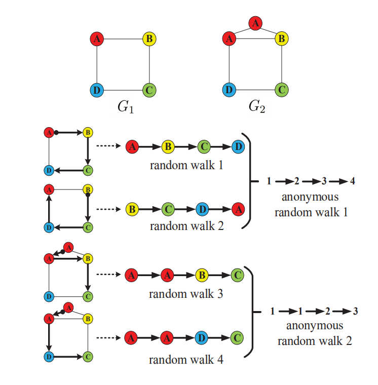
Example. Random walks , , and sampled from and in Figure 2 are completely different. However, in anonymous random walks view, the new label for each node is redefined as the position of the first occurrence of node with same label in the random walk sequence. This makes the initial four different random walks be changed into two anonymous random walks, and .
As shown in Figure 3, all different random walks with length in and from Figure 2 will be converted into only anonymous random walks. Random walks record the labels information of nodes traveled, under sufficient samples, they can accurately capture structure traits and reconstructure the original graph. But over precise information will not be efficient to capture graph structure features because of sparse distribution over all random walks. Anonymous random walks translate random walks into a sequence of integers recording first appearing positions.

4.1.2 Skeleton
We draw independently a set of random walks with length on in graphs set , and calculate its anonymous random walks .
For a large graph , to count all possible anonymous random walks needs vast computational resources. However, sampling random walks with length to approximate actual distribution of anonymous random walks, the overall computing running time will be [16]. The relation of estimation of samples number and the number of anonymous random walks is determined by hyperparameters and [20]:
| (7) |
Next we tend to leverage vectors to represent whether some specific anonymous random walks contained in a graph or not.
Definition 6 (Skeleton). Given graphs set , we sample random walks with length on each graph in and integrate them as set . The correspond anonymous random walks set has unequal elements. The skeleton of graph is defined as an shape vector , where
| (8) |
4.2 Component Module
Component module uses a more flexible approach to capture similarity between two graphs by frequent patterns, for example, itemsets, subsequences, or subgraphs, which appear in a data set with frequency no less than a user-specified minimum support () threshold. Component module basically includes three steps: (1) mining frequent subgraphs, (2) selecting features, (3) learning component features.
4.2.1 Frequent Subgraph
Definition 7 (Subgraph). A graph is called a subgraph of a graph if nodes satisfy V() V() and edges satisfy E() E().

Two graphs are similar if their subgraphs are similar since subgraphs have been recognized as fundamental units and are building blocks for complex networks [21]. But usually only a fraction of the large amount number of subgraphs are actually relevant to data mining problems. Our methodology focus on mining subgraphs of different proportion in graph set, and then embed these distribution features into graph component representation.
Definition 8 (Frequent Subgraph). Let be a subgraph in subgraphs set mined from , and will be called frequent subgraph if , where is the threshold, , and is called the of .
Example. We still take , in Figure 2 and subgraphs , , in Figure 4 as examples. If we set threshold , only subgraphs can be regarded as frequent subgraph. However, if we set threshold , all of , and will be regarded frequent.
Frequent pattern, as a form of non-linear feature combinations over the set of different subgraphs, has higher discriminative power than that of single kind of subgraph because they capture more underlying semantics of the data. The key point is to specify the hyperparameter threshold used in model in frequent pattern, and we will study the influence of for machine learning tasks in Section 5. If an infrequent feature is used, the model cannot generalize well to the test data since it is built based on statistically minor observations, hence the discriminative power of low-support features will be limited [22].

4.2.2 Component
To mine all frequent subgraphs will face two challenges: (1) The time complexity which is dominated by the overall nodes number of each graph, makes it computational infeasible to find all subgraphs. (2) In analogue of graph isomorphism checking in which two graphs have different sizes, subgraph isomorphism checking has been proven to be NP-complete [23]. A slightly less restrictive measure of similarity can be defined based on the size of the largest common subgraph in two graphs, but unfortunately the problem of finding the largest common subgraph of two graphs is NP-complete as well [23].
To tackle with such two challenges above, gSpan [24] algorithm builds a new lexicographic order among graphs, and maps each graph to a unique minimum DFS-code as its canonical label. Based on this lexicographic order among DFS-code, gSpan adopts the depth-first search strategy to discover frequent subgraphs efficiently. Repeating this procedure until either when the of a graph is less than threshold , or its code is not a minimum code, which means this graph and all its descendants have been generated and discovered before. Now we give the definition of component to indicate what frequent subgraphs mined by gSpan graph has.
Definition 9 (Component). Given a set of graphs and threshold , all different frequent subgraphs obtained by gSpan are contained in set = . The component of is defined as an shape vector , where
| (9) |
4.3 TRAINING
For graph data set , supposed that all anonymous random walks with length mined are in and all frequent subgraphs mined under threshold are in , we leverage PV-DBOW to learn graphs embedding matrix whose each row is an embedding for each graph, anonymous random walks matrix whose each row is an embedding for each anonymous random walk and frequent subgraphs matrix whose each row is an embedding for each frequent subgraph. Vectors and are corresponding skeleton and component for graph , .
Graphs embedding matrix has size, matrix is in size and matrix is in size, where is embedding dimension. PV-DBOW treats graph data set as a documents set, each graph in as a document and each substructure mined in as a word contained in a document.
To begin with, we focus on anonymous random walks and seek to optimize the following objective function, which maximizes the log-probability of predicting anonymous random walks that appear in graph :
| (10) |
where is an binary vector whose -th column element is and -th column element equals to if .
The probability is defined as a softmax unit parametrized by a dot product of and which are embedding vectors of and :
| (11) |
Next, we use same method to maximize the log-probability of predicting the frequent subgraphs that appear in graph :
| (12) |
where is an binary vector whose -th column element is and -th column element equals to if .
The probability is defined as a softmax function parametrized by a dot product of and which are embedding vectors of subgraph and :
| (13) |
We yield its loss function as following:
| (15) |
where is sigmoid function.
The last two items in equation (15) which sum over all anonymous random walks and subgraphs directly, are too expensive since and usually tend to be very large. Hence we proceed with an approximation by negative sampling to make the optimization problem tractable. The normalization terms from the softmax are replaced by anonymous random walks negative samples from but not contained in and frequent subgraphs negative samples from but not contained in . Thus equation (15) can be rewritten as:
| (16) |
where and are the embedding vectors of samples and respectively, and belongs to when , is in when .
Finally, we optimize loss function (16) with stochastic gradient descent and update . After the learning process finishes, two graphs are near in embedding space if they have similar skeleton and component, and we summarize this training process in Algorithm 3.
5 EXPERIMENTS
In this section, to quantitatively evaluate classification capability of our model, we conduct extensive experiments on a variety of widely-used datasets to compare with several state-of-the-art baselines.
5.1 DATASETS
We evaluate our proposed method on binary classification task using seven real-world graph datasets whose statictics are summarized in Table 1. MUTAG [25] is a dataset of aromatic and heteroaromatic nitro compounds labeled according to whether or not they have a mutagenic effect on bacteria. PROTEINS [26] is a set of proteins graphs where nodes represent secondary structure elements and edges indicate neighborhood in the amino-acid sequence or in 3-dimension space. ENZYMES [26] consists of protein tertiary structures obtained from the BRENDA enzyme database. DD [27] is a dataset of protein structures where nodes represent amino acids and edges indicate spatial closeness, which are classified into enzymes or non-enzymes. PTC-MR [28] consists of graph representations of chemical molecules labeled according to carcinogenicity on rodents. NCI-1, NCI-109 [1] are datasets of chemical compounds divided by the anti-cancer property (active or negative). These datasets have been made publicly available by the National Cancer Institute (NCI).
| Datasets | Graph | Class | Average Node | Average Edge |
|---|---|---|---|---|
| MUTAG | 188 | 2 | 17.93 | 19.79 |
| DD | 1178 | 2 | 284.32 | 715.66 |
| PTC-MR | 344 | 2 | 14.29 | 14.69 |
| NCI-1 | 4110 | 2 | 29.87 | 32.30 |
| NCI-109 | 4127 | 2 | 29.68 | 32.13 |
| PROTEINS | 1113 | 2 | 39.06 | 72.82 |
| ENZYMES | 600 | 6 | 32.63 | 64.14 |
5.2 BASELINES
In order to demonstrate the effectiveness of our proposed approach, we compare it with several baseline methods, all of which utilize the entire graph for feature extraction. These competitors can be categorized into four main groups:
- 1.
Graph kernels based methods: The shortest path (SP) [11] kernel measures the similarity of a pair of graphs by comparing the distance of the shortest paths between nodes in the graphs. Graphlet kernel (GK) [20] measures graph similarity by counting the number of different graphlets and Deep GK [29] is deep graphlet kernel. Weisfeiler-Lehman kernel (WL) [5] uses subtree pattern to mine structure information and Deep WL [29] is deep Weisfeiler-Lehman kernel.
- 2.
Unsupervised graph embedding methods: node2vec [4] is an unsupervised task agnostic method that learns entire graph embedding. It proposes every graph into a fixed size vector containing distributed representation of graph structures.
- 3.
Supervised graph embedding methods: PSCN [8] is a convolutional neural network algorithm which has achieved strong classification accuracy in many datasets.
- 4.
Unsupervised graph embedding methods: AWE [13] uses an anonymous random walks approach to embed entire graphs in an unsupervised manner.
| Algorithm | MUTAG | DD | PTC-MR | NCI-1 | NCI-109 | PROTEINS | ENZYMES |
|---|---|---|---|---|---|---|---|
| WL | 80.63 (3.07) | 77.95 (0.70) | 56.97 (2.01) | 80.13 (0.50) | 80.22 (0.34) | 72.92 (0.56) | 53.15 (1.14) |
| Deep WL | 82.95 (1.96) | - | 59.17 (1.56) | 80.31 (0.46) | 80.32 (0.33) | 73.30 (0.82) | 53.43 (0.91) |
| GK | 81.66 (2.11) | 78.45 (0.26) | 57.26 (1.41) | 62.28 (0.29) | 62.60 (0.19) | 71.67 (0.55) | 26.61 (0.99) |
| Deep GK | 82.66 (1.45) | - | 57.32 (1.13) | 62.48 (0.25) | 62.69 (0.23) | 71.68 (0.50) | 27.08 (0.79) |
| graph2vec | 83.15 (9.25) | 58.64 (0.01) | 60.17 (6.86) | 73.22 (1.81) | 74.26 (1.47) | 73.30 (2.05) | 44.33 (0.09) |
| PSCN | 92.63 (4.21) | 77.12 (2.41) | 60.00 (4.82) | 78.59 (1.89) | - | 75.89 (2.76) | - |
| AWE | 87.87 (9.76) | 71.51 (4.02) | 59.14 (1.83) | 62.72 (1.67) | 63.21 (1.42) | 70.01 (2.52) | 35.77 (5.93) |
| GraphCSC | 88.42 (6.47) | 89.38 (2.73) | 64.04 (3.61) | 85.70 (4.29) | 85.46 (3.66) | 76.71 (3.06) | 57.21 (5.70) |
| 0.15 | 0.25 | 0.75 | 0.20 | 0.20 | 0.60 | 0.55 | |
| dim | 128 | 8 | 128 | 16 | 16 | 32 | 128 |


5.3 Evaluation Metrics
To evaluate the performance of GraphCSC, we randomly split the data into roughly equal-size parts and perform a -fold cross validation on each dataset, in which folds for training and fold as validation for testing. This process is repeated times and an average accuracy is reported as prediction. Since we focus on graph embedding not on a classifier, we feed the embedding vectors to Support Vector Machine (SVM) with RBF kernel function with parameter varing from the range .
5.4 Parameter sensitivity
Since we tend to prove that the performance of our model GraphCSC may have a gain on experiments results than method only considers skeletons, thus to explore how the hyperparameters in skeleton module affect tasks performace will not be our priority. For the need of brevity, the length is set as to generate a corpus of co-occurred anonymous random walks for all given datasets. To approximate actual distribution of anonymous random walks, we follow [13] to set the sampling hyperparameters and . In order to evaluate how the parameters sensitivity of threshold and embedding dimensions affect the classification performance of GraphCSC on datasets, all parameters are assumed to be default except and .
We first conduct experiments with , then assess the classification accuracy as a function of threshold for different datasets. Best performance is indicated with red mark in Figure 6. Then in Figure 7, experiments examine the influence of varying the from with the best s obtained from Fig.5. The best accuracy is also signed in red as shown in each figure.
5.5 Results and Discussion
The average classification accuracy (standard deviation) over 10-fold cross-validation of GraphCSC (with and that lead to optimal result from Figure 6 and Figure 7, and baselines on seven real-world datasets are summarized in Table 2. From the results, it is evidently shown that GraphCSC is always the best in terms of performance on 6 datasets with exception on MUTAG, where GraphCSC gets second best result. More specifically, the proposed model achieves improvement over graph kernals based methods (WL, Deep WL, GK and Deep GK), and is competitive against graph embedding method (graph2vec) with gain in accuracy. However, supervised graph embedding method PSCN is more superior with 4.21% higher in accuracy in MUTAG dataset classification. It is also obvious that GraphCSC outperforms AWE approach in every single dataset. This significantly demonstrates the effectiveness of the proposed model on classification tasks due to having access to skeleton and component features, which enable GraphCSC to get more complex structures information, while AWE processes only fixed size skeletons instead.
Figure 6 presents the classification accuracy of increasing threshold . In MUTAG and NCI-1, experiments get best performance when and separately. Then results decrease slowly and maintain stable, after reaching (for MUTAG) and (for NCI-1), lines drop rapidly until getting to another flat states. A common phenomenon is that for DD, PROTEINS and ENZYMES, accuracy lines increase from the beginnings and decrease slowly after meeting the tops. Another observation is that in PTC-MR, performance has 2 closed top best results when and , while the result at has only gain over that at . It is very interesting that threshold centers around a low value for most datasets. A possible explanation is that low will lead to more sufficient frequent subgraphs which will provide adequate complementary structure information for pattern just uses skeletons. As a consequence, this enforces model’s discriminate power.
Figure 7 examines the effects of embedding dimension hyperparameter . As we can see from the figure, in MUTAG and PROTEINS, there is a relatively gentle first-increasing and then-decreasing accuracy line when increases. We note that for DD, the performance line goes down slowly and maintains stable at around and then again falls quickly. Accuracy in ENZYMES changes roughly, indicating that classification result significantly suffers from embedding dimension . While it seems that has no clearly effects on classification results for PTC-MR and NCI-1. The beat s for MUTAG and ENZYMES center at 128, but the values tend to be small (usually no more than 32) in DD, PTC-MR, NCI-1 and PROTEINS, we can infer that small s would reflect more obvious features for these 4 datasets.
6 Conclusion
In this paper, we focus to study the problem of graph classification and propose GraphCSC, a new methodology that learns graph representation from horizontal and vertical perspectives to mine graph structures, i.e., skeletons and components. And our model is demonstrated to be superior to approach which utilizes only skeletons. Our method treats a graph as a document and different substructures or subgraphs in it as words by NLP framework PV-DBOW, thus the graph embedding GraphCSC learns integrate various size structures information. Several real-world graph classification tasks show that our model can achieve promising performances than a list of state-of-art baselines.
For future work, an interesting problem needs to be study further. We tend to fucus on more complex graph structures, for example, clusters. Since a cluster usually contains dozens or even hundreds of nodes and edges, there may show more valuable features which may reflect more implicit graph properties. We would also like to investigate graph embedding with mixed structures from low-order subgraphs to big clusters, and to verify whether this would be helpful for better results than GraphCSC.
Acknowledgements
This work is supported by the Fundamental Research Funds for the Central Universities, the National Natural Science Foundation of China (No.11201019), the International Cooperation Project No.2010DFR00700, Fundamental Research of Civil Aircraft No. MJ-F-2012-04, the Beijing Natural Science Foundation (1192012, Z180005) and National Natural Science Foundation of China (No.62050132).
References
- [1] J. B. Lee, R. Rossi, X. Kong, Graph classification using structural attention, in: Proceedings of the 24th ACM SIGKDD International Conference on Knowledge Discovery & Data Mining, 2018, pp. 1666–1674.
- [2] L. Backstrom, J. Leskovec, Supervised random walks: predicting and recommending links in social networks, in: the Fourth International Conference on Web Search and Web Data Mining, 2011, p. 635–644.
- [3] F. Costa, K. D. Grave, Fast neighborhood subgraph pairwise distance kernel, in: International Conference on International Conference on Machine Learning, 2010.
- [4] M. Niepert, M. Ahmed, K. Kutzkov, Learning convolutional neural networks for graphs, in: International conference on machine learning, 2016, pp. 2014–2023.
- [5] N. Shervashidze, P. Schweitzer, E. Jan, V. Leeuwen, K. M. Borgwardt, Weisfeiler-lehman graph kernels, Journal of Machine Learning Research 1 (3) (2010) 1–48.
- [6] Z. Wu, S. Pan, F. Chen, G. Long, P. S. Yu, A comprehensive survey on graph neural networks, IEEE Transactions on Neural Networks and Learning Systems PP (99) (2020) 1–21.
- [7] A. Krizhevsky, I. Sutskever, G. E. Hinton, Imagenet classification with deep convolutional neural networks, in: Advances in neural information processing systems, 2012, pp. 1097–1105.
- [8] T. N. Kipf, M. Welling, Semi-supervised classification with graph convolutional networks, arXiv preprint arXiv:1609.02907.
- [9] J. Hartmanis, Computers and intractability: a guide to the theory of np-completeness (michael r. garey and david s. johnson), Siam Review 24 (1) (1982) 90.
- [10] H. Kashima, K. Tsuda, A. Inokuchi, Marginalized kernels between labeled graphs, in: Proceedings of the 20th international conference on machine learning (ICML-03), 2003, pp. 321–328.
- [11] K. M. Borgwardt, H.-P. Kriegel, Shortest-path kernels on graphs, in: Fifth IEEE international conference on data mining (ICDM’05), IEEE, 2005, pp. 8–pp.
- [12] R. Kondor, N. Shervashidze, K. M. Borgwardt, The graphlet spectrum, in: Proceedings of the 26th Annual International Conference on Machine Learning, 2009, pp. 529–536.
- [13] S. Ivanov, E. Burnaev, Anonymous walk embeddings, arXiv preprint arXiv:1805.11921.
- [14] S. Micali, Z. A. Zhu, Reconstructing markov processes from independent and anonymous experiments, Discrete Applied Mathematics 200 (2016) 108–122.
- [15] D. Nguyen, W. Luo, T. D. Nguyen, S. Venkatesh, D. Phung, Learning graph representation via frequent subgraphs, in: Proceedings of the 2018 SIAM International Conference on Data Mining, SIAM, 2018, pp. 306–314.
- [16] Q. Le, T. Mikolov, Distributed representations of sentences and documents, in: International conference on machine learning, 2014, pp. 1188–1196.
- [17] T. Mikolov, Distributed representations of words and phrases and their compositionality, Advances in Neural Information Processing Systems 26 (2013) 3111–3119.
- [18] A. Mnih, G. E. Hinton, A scalable hierarchical distributed language model, in: Advances in neural information processing systems, 2009, pp. 1081–1088.
- [19] F. Rousseau, E. Kiagias, M. Vazirgiannis, Text categorization as a graph classification problem, in: Proceedings of the 53rd Annual Meeting of the Association for Computational Linguistics and the 7th International Joint Conference on Natural Language Processing (Volume 1: Long Papers), 2015, pp. 1702–1712.
- [20] N. Shervashidze, S. Vishwanathan, T. Petri, K. Mehlhorn, K. Borgwardt, Efficient graphlet kernels for large graph comparison, in: Artificial Intelligence and Statistics, 2009, pp. 488–495.
- [21] R. Milo, S. Shen-Orr, S. Itzkovitz, N. Kashtan, D. Chklovskii, U. Alon, Network motifs: simple building blocks of complex networks, Science 298 (5594) (2002) 824–827.
- [22] C. Hong, Towards accurate and efficient classification: A discriminative and frequent pattern-based approach, Ph.D. thesis, University of Illinois at Urbana-Champaign. (2008).
- [23] M. J. Zaki, W. Meira, Data mining and analysis: fundamental concepts and algorithms, Cambridge University Press, 2014.
- [24] X. Yan, J. Han, gspan: Graph-based substructure pattern mining, in: 2002 IEEE International Conference on Data Mining, 2002. Proceedings., IEEE, 2002, pp. 721–724.
- [25] A. K. Debnath, R. L. L. D. Compadre, G. Debnath, A. J. Shusterman, C. Hansch, Structure-activity relationship of mutagenic aromatic and heteroaromatic nitro compounds. correlation with molecular orbital energies and hydrophobicity., Journal of Medicinal Chemistry 34 (2) (1991) 786–797.
- [26] K. M. Borgwardt, O. C. Soon, S. Stefan, S. V. N. Vishwanathan, A. J. Smola, K. Hans-Peter, Protein function prediction via graph kernels, Bioinformatics 21 (suppl_1) (2005) i47–i56.
- [27] P. D. Dobson, A. J. Doig, Distinguishing enzyme structures from non-enzymes without alignments, Journal of Molecular Biology 330 (4) (2003) 771–783.
- [28] C. Helma, R. D. King, S. Kramer, A. Srinivasan, The predictive toxicology challenge 2000-2001, Bioinformatics 17 (1) (2001) 107–108.
- [29] P. Yanardag, S. Vishwanathan, Deep graph kernels, in: Proceedings of the 21th ACM SIGKDD International Conference on Knowledge Discovery and Data Mining, 2015, pp. 1365–1374.