Joint Transmit Precoding and Reflect Beamforming Design for IRS-Assisted MIMO Cognitive Radio Systems

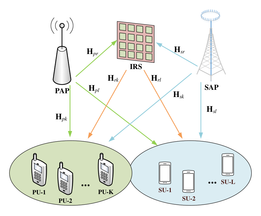
We consider the IRS-MIMO-CR system, as shown in Fig. 1, where a secondary access point (SAP) serves multiple secondary users (SUs) without affecting the communications between primary access point (PAP) and multiple primary users (PUs) in the primary network. All nodes are equipped with multiple antennas and the number of antennas at the PAP, PUs, SAP and SUs are $N_{PA}$, $N_{PU}$, $N_{SA}$ and $N_{SU}$, respectively. Denote the sets of PUs and SUs as ${\cal K}=\left\{{1,2,...,K}\right\}$ and ${\cal L}=\left\{{1,2,...,L}\right\}$, respectively. In addition, an IRS composed of $M$ passive elements, which are denoted as the set ${\cal M}=\{1,2,...,M\}$, is installed on a surrounding wall to assist the communications between the SAP and SUs. The IRS has a smart controller, who has the capability of dynamically adjusting the phase shift of each reflecting element based on the propagation environment learned through periodic sensing [7].

The number of data streams for each SU is assumed as $d$, satisfying $1\leq d\leq\min\left\{N_{SA},N_{SU}\right\}$. The transmit signal from the SAP is given by

where $\bm{s}_{l}\in{\mathbb{C}^{d\times 1}},\forall l\in{\cal L}$ is the $d\times 1$ data symbol vector designated for the $l$th SU satisfying $\mathbb{E}\left[\bm{s}_{l}\bm{s}_{l}^{H}\right]=\mathbf{I}$ and $\mathbb{E}\left[\bm{s}_{i}\bm{s}_{j}^{H}\right]=\bm{0},\forall i,j\in{\cal L},i\neq j$. In addition, $\mathbf{F}_{l}\in\mathbb{C}^{N_{SA}\times d},\forall l\in{\cal L}$ is the linear precoding matrix used by the SAP for the $l$th SU. As a result, the received signals, which are transmitted from SAP, at the $k$th PU and $l$th SU are given by

where $\bm{r}_{k}\in\mathbb{C}^{N_{PU}\times 1},\forall k\in{\cal K}$ stands for the signal which is transmitted from PAP and received by the $k$th PU. Moreover, the baseband equivalent channels from the SAP to the $k$th PU, from the SAP to the $l$th SU, from the SAP to the IRS, from the IRS to the $k$th PU, from the IRS to the $l$th SU are modelled by matrices $\mathbf{H}_{sk}\in\mathbb{C}^{{N_{PU}}\times{N_{SA}}}$, $\mathbf{H}_{sl}\in\mathbb{C}^{{N_{SU}}\times{N_{SA}}}$, $\mathbf{H}_{sr}\in\mathbb{C}^{M\times{N_{SA}}}$, $\mathbf{H}_{rk}\in\mathbb{C}^{{N_{PU}}\times M}$ and $\mathbf{H}_{rl}\in\mathbb{C}^{{N_{SU}}\times M}$, respectively. Let $\mathbf{\Theta}=diag({\bm{\theta}})\in{\mathbb{C}^{M\times M}}$ denote the diagonal reflection matrix of the IRS, with $\bm{\theta}={\left[\theta_{1},\theta_{2},...,\theta_{M}\right]^{T}}\in{\mathbb{C}^{M\times 1}}$ and $\left|\theta_{m}\right|=1,\;\forall m\in{\cal M}$. Therefore, the effective MIMO channel matrix from the SAP to the $k$th PU and $l$th SU receiver is given by ${\mathbf{G}_{sk}}\left(\mathbf{\Theta}\right)={\mathbf{H}_{sk}}+{\mathbf{H}_{rk}}\mathbf{\Theta}{\mathbf{H}_{sr}}$ and ${\mathbf{G}_{sl}}\left(\mathbf{\Theta}\right)={\mathbf{H}_{sl}}+{\mathbf{H}_{rl}}\mathbf{\Theta}{\mathbf{H}_{sr}}$, respectively. $\bm{n}_{k}\sim CN\left(\bm{0},\sigma_{k}^{2}\mathbf{I}\right)$ represents the additive white Gaussian noise at the $k$th PU, and $\bm{n}_{l}\sim CN\left(\bm{0},\sigma_{l}^{2}\mathbf{I}\right)$ is the equivalent noise at the $l$th SU, which captures the joint effect of the received interference from the primary network and thermal noise. $\sigma_{k}^{2}$ and $\sigma_{l}^{2}$ denote the corresponding average noise power at the $k$th PU and the $l$th SU. By substituting (1) into (3), the received signals of the $l$th SU are reformulated as follows

Denotes the collection of precoding matrixs used by the SAP as $\mathbf{F}=\left\{\mathbf{F}_{1},\mathbf{F}_{2},...,\mathbf{F}_{L}\right\}$. Hence, the transmit data rate (bit/s/Hz) of the $l$th SU is written as follows

where $\mathbf{J}_{l}=\sum\limits_{i=1,i\neq l}^{L}{\mathbf{G}_{sl}\left(\mathbf{\Theta}\right)\mathbf{F}_{i}\mathbf{F}_{i}^{H}\mathbf{G}_{sl}^{H}\left(\mathbf{\Theta}\right)}+\sigma_{l}^{2}\mathbf{I}$ represents the interference-plus-noise covariance matrix of the $l$th SU. Moreover, the interference signal power imposed on the $k$th PU is denoted by

As mentioned earlier, we discuss the joint optimization of the transmit precoding matrix at the SAP and the reflection coefficients at the IRS to maximize the achievable WSR of SUs, subject to the total transmit power constraint at the SAP, interference constraints at PUs and the reflection coefficient constraint at the IRS. Thus we have the following OP1,

Herein, C1 characterizes the total transmit power constraint at the SAP, C2 defines the interference constraints at PUs, and C3 represents the IRS reflecting coefficient constraint, $\Gamma_{k}$ denotes the maximum received interference power at the PU $k$. It is evident that OP1 is a non-convex nonlinear programming with coupled variables $\mathbf{F}$ and $\mathbf{\Theta}$ and also the uni-modular constraint on each reflection coefficient $\mathbf{\Theta}_{mm}$, which makes it difficult to solve. Therefore, in the sequel, we pursue the suboptimal approach to handle OP1.

To deal with the complex objective function, we reformulate OP1 by employing the well-known WMMSE [32] method. Specifically, the linear decoding matrix is applied to estimate the signal vector for each SU, which is denoted by

where $\mathbf{U}_{l}\in\mathbb{C}^{{N_{SU}}\times d}$ is the decoding matrix for the $l$th SU. Then, the MSE matrix for the $l$th SU is given by

where $\bm{s}$ and $\bm{n}$ denote the collections of data symbols and noise vectors of all SUs, respectively. Denoting the sets of decoding matrices as $\mathbf{U}=\left\{\mathbf{U}_{l},\;\forall l\in{\cal L}\right\}$ and introducing a set of auxiliary matrices $\mathbf{W}=\left\{\mathbf{W}_{l}\succcurlyeq\mathbf{0},\;\forall l\in{\cal L}\right\}$, OP1 can be reformulated as the following OP2

Herein, ${h_{l}}\left(\mathbf{W},\mathbf{U},\mathbf{F},\mathbf{\Theta}\right)$ is given by

Note that, by iteratively obtaining one set of variables while keeping the others fixed, the objective function in OP2 is much easier to handle with AO. Since the decoding matrices $\mathbf{U}$ and auxiliary matrices $\mathbf{W}$ only appear in ${h_{l}}\left(\mathbf{W},\mathbf{U},\mathbf{F},\mathbf{\Theta}\right)$, the optimal solution of $\mathbf{U}$ and $\mathbf{W}$ can be obtained by setting the first-order derivative of ${h_{l}}\left(\mathbf{W},\mathbf{U},\mathbf{F},\mathbf{\Theta}\right)$ with respect to $\mathbf{U}_{l}$ and $\mathbf{W}_{l}$ to zero while keeping the other matrices fixed. Hence, the optimal solutions are denoted by

Herein, given the reflection coefficient matrix $\mathbf{\Theta}$ at the IRS, $\mathbf{G}_{sl}\left(\mathbf{\Theta}\right)$ is simplistically denoted as $\mathbf{G}_{sl}$. Moreover, $\mathbf{\hat{E}}_{l}$ is obtained by inserting $\mathbf{\hat{U}}_{l}$ into the MSE matrix of the $l$th SU, yielding

In the following, the precoding matrices $\mathbf{F}$ and reflection coefficient matrix $\mathbf{\Theta}$ are optimized with given $\mathbf{U}$ and $\mathbf{W}$.

In this subsection, we discuss the precoding matrices optimization at the SAP given the reflecting coefficients at the IRS, decoding matrices and auxiliary matrices. Hence, by substituting $\mathbf{E}$ into the objective function of OP2 and discarding the constant terms, the precoding matrices optimization problem can be transformed as the following OP3,

In which, $\mathbf{G}_{sk}$ is the abbreviated form of $\mathbf{G}_{sk}\left(\mathbf{\Theta}\right)$ with given the reflection coefficient matrix $\mathbf{\Theta}$ at the IRS. In addition, ${\mathbf{X}_{0}}=\sum\limits_{m=1}^{L}{\omega_{m}}\mathbf{G}_{sm}^{H}{\mathbf{U}_{m}}{\mathbf{W}_{m}}\mathbf{U}_{m}^{H}{\mathbf{G}_{sm}}\succcurlyeq\mathbf{0}$, ${\mathbf{X}_{k}}=\mathbf{G}_{sk}^{H}{\mathbf{G}_{sk}}\succcurlyeq\mathbf{0},\;\forall k\in{\cal K}$ and ${\mathbf{Y}_{l}}={\omega_{l}}{\mathbf{W}_{l}}\mathbf{U}_{l}^{H}{\mathbf{G}_{sl}},\;\forall l\in{\cal L}$. It is obvious that OP3 is quadratically constrained quadratic programming (QCQP) problem [33]. Since $\mathbf{X}_{0}\succcurlyeq\mathbf{0}$ and $\mathbf{X}_{k}\succcurlyeq\mathbf{0}$, OP3 is convex and can be easily solved with standard interior-point methods.

In this subsection, given the precoding matrices at the SAP, decoding matrices and auxiliary matrices, the optimization of the reflecting coefficient matrix $\mathbf{\Theta}$ at IRS is discussed. Particularly, we have the following OP4:

where ${\mathbf{Q}_{s}}=\sum\limits_{m=1}^{L}{{\mathbf{F}_{m}}\mathbf{F}_{m}^{H}}$. By applying ${\mathbf{G}_{sl}}\left(\mathbf{\Theta}\right)={\mathbf{H}_{sl}}+{\mathbf{H}_{rl}}\mathbf{\Theta}{\mathbf{H}_{sr}}$, we have

Based on the above conversions, by discarding the constant terms, OP4 can be transformed into the following formulation,

Herein, ${\mathbf{B}_{0}}=\sum\limits_{l=1}^{L}{{\omega_{l}}\mathbf{H}_{rl}^{H}{\mathbf{U}_{l}}{\mathbf{W}_{l}}\mathbf{U}_{l}^{H}{\mathbf{H}_{rl}}}\succcurlyeq\mathbf{0}$, ${\mathbf{B}_{k}}=\mathbf{H}_{rk}^{H}{\mathbf{H}_{rk}}\succcurlyeq\mathbf{0}$, $\mathbf{C}={\mathbf{H}_{sr}}{\mathbf{Q}_{s}}\mathbf{H}_{sr}^{H}\succcurlyeq\mathbf{0}$, ${\mathbf{D}_{0}}=\sum\limits_{l=1}^{L}{{\omega_{l}}{\mathbf{H}_{sr}}{\mathbf{Q}_{s}}\mathbf{H}_{sl}^{H}{\mathbf{U}_{l}}{\mathbf{W}_{l}}\mathbf{U}_{l}^{H}{\mathbf{H}_{rl}}}-\sum\limits_{l=1}^{L}{{\omega_{l}}{\mathbf{H}_{sr}}{\mathbf{F}_{l}}{\mathbf{W}_{l}}\mathbf{U}_{l}^{H}{\mathbf{H}_{rl}}}$, ${\mathbf{D}_{k}}={\mathbf{H}_{sr}}{\mathbf{Q}_{s}}\mathbf{H}_{sk}^{H}{\mathbf{H}_{rk}}$ and ${\tilde{\Gamma}_{k}}={\Gamma_{k}}-{\rm{Tr}}\left({{\mathbf{H}_{sk}}{\mathbf{Q}_{s}}\mathbf{H}_{sk}^{H}}\right)$. Since $\mathbf{\Theta}=diag({\bm{\theta}})$ is a diagonal matrix, by adopting the matrix identity in [34], it follows that

Further, denote ${{\bm{d}}_{0}}={\left[{{{\left[{{\mathbf{D}_{0}}}\right]}_{1,1}},{{\left[{{\mathbf{D}_{0}}}\right]}_{2,2}},...,{{\left[{{\mathbf{D}_{0}}}\right]}_{M,M}}}\right]^{T}}$ and ${{\bm{d}}_{k}}={\left[{{{\left[{{\mathbf{D}_{k}}}\right]}_{1,1}},{{\left[{{\mathbf{D}_{k}}}\right]}_{2,2}},...,{{\left[{{\mathbf{D}_{k}}}\right]}_{M,M}}}\right]^{T}}$ as the collections of diagonal elements of $\mathbf{D}_{0}$ and $\mathbf{D}_{k}$. We thus have

Therefore, the problem (20) can be simplified as follows

Herein, since $\mathbf{B}_{0}\succcurlyeq\mathbf{0}$, $\mathbf{B}_{k}\succcurlyeq\mathbf{0}$ and $\mathbf{C}\succcurlyeq\mathbf{0}$, we have $\mathbf{\Upsilon}_{0}=\mathbf{B}_{0}\odot\mathbf{C}^{T}\succcurlyeq\mathbf{0}$ and $\mathbf{\Upsilon}_{k}=\mathbf{B}_{k}\odot\mathbf{C}^{T}\succcurlyeq\mathbf{0}$. However, due to the non-convexity of the uni-modulus constraint on each reflection coefficient $\bm{\theta}_{m}$, the problem (23) is non-convex. Hence, penalty function (PF) and successive convex approximation (SCA) are adopted. Specifically, introducing the slack factor $\lambda\leq 0$, the problem (23) can be reformulated as follows

The term $\lambda\bm{\theta}^{H}\bm{\theta}$ could ensure that the uni-modulus constraint $\left|\bm{\theta}_{m}\right|=1,\;\forall m\in{\cal M}$ is hold at the optimal solution when $\lambda\to+\infty$. Note that, the objective function of the problem (24) is the sum of a convex function and a concave function which means (24) is non-convex. Hence, the SCA-based algorithm [35, 36] is used to handle (24) and the concave part of the objective function is approximated by its first order Taylor expansion. In specific, given the initial point $\bm{\theta}^{(n)}$ and by discarding the constant terms, the sub-problem can be denoted by

Now, (25) is convex and can be solved by standard interior-point methods [33]. Therefore, (24) can be tackled by solving a series of convex problems iteratively and the details are summarized in Algorithm 1 as below.

Based on the above discussion, we formulate the PF-based algorithm to solve the OP4 as the following Algorithm 2.

Note that, we adopt the stopping criterion $\sum\limits_{m=1}^{M}{{\left({\left|\bm{\hat{\theta}}_{m}^{(n)}\right|-1}\right)}^{2}}\leq\varepsilon$ to ensure the uni-modulus constraint holds at the optimal solution for Algorithm 2.

In this subsection, the overall algorithm for OP1 is provided. As mentioned, the algorithm is based on alternating optimization, which optimizes the objective function with respect to different subsets of optimization variables in each iteration while the other subsets are fixed. Therefore, it is summarized as the following Algorithm 3.

In this subsection, we discuss the precoding matrices optimization at the SAP for given the reflecting coefficients at the IRS, decoding matrices and auxiliary matrices. Hence, substituting $\mathbf{E}$ into the objective function of OP6 and discarding the constant terms, the precoding matrices optimization problem can be transformed as the following OP7,

Herein, $\mathbf{G}_{sp}$ is the abbreviated form of $\mathbf{G}_{sp}\left(\mathbf{\Theta}\right)$ with given the reflection coefficient matrix $\mathbf{\Theta}$ at the IRS. In addition, ${\mathbf{X}_{0}}=\sum\limits_{m=1}^{L}{\omega_{m}}\mathbf{G}_{sm}^{H}{\mathbf{U}_{m}}{\mathbf{W}_{m}}\mathbf{U}_{m}^{H}{\mathbf{G}_{sm}}\succcurlyeq\mathbf{0}$, ${\mathbf{X}_{p}}=\mathbf{G}_{sp}^{H}{\mathbf{G}_{sp}}\succcurlyeq\mathbf{0}$ and ${\mathbf{Y}_{l}}={\omega_{l}}{\mathbf{W}_{l}}\mathbf{U}_{l}^{H}{\mathbf{G}_{sl}},\;\forall l\in{\cal L}$. Same as OP3, since $\mathbf{X}_{0}\succcurlyeq\mathbf{0}$ and $\mathbf{X}_{p}\succcurlyeq\mathbf{0}$, OP7 is QCQP convex optimization problem [33], which can be solved by the standard convex solver packages such as CVX. However, the computational complexity is high. In the following, we provide a low-complexity SCA-based algorithm which can obtain the optimal solution of the OP7 by solving a series of simple convex problem with Lagrangian dual decomposition method. For which, we introduce the following proposition.

Proposition 1: Let $f_{p}\left(\mathbf{F}\right)=\sum\limits_{l=1}^{L}{Tr\left({\mathbf{F}_{l}^{H}{\mathbf{X}_{p}}{\mathbf{F}_{l}}}\right)}$, ${\mathbf{X}_{p}}\succcurlyeq\mathbf{0}$, $\mathbf{Z}_{p}={\lambda}_{p}\mathbf{I}$ and ${\lambda}_{p}$ denotes the maximum eigenvalue of the $\mathbf{X}_{p}$. Then for $\forall\mathbf{F}$ and given $\mathbf{F}^{(n)}$, there exists

which satisfies the following three conditions:

1) ${\tilde{f}_{p}}\left({{\mathbf{F}^{(n)}}|{\mathbf{F}^{(n)}}}\right)={f_{p}}\left({{\mathbf{F}^{(n)}}}\right)$,

2) ${\left.{{\nabla_{{\mathbf{F}}^{*}}}{{\tilde{f}}_{p}}\left({\mathbf{F}|{\mathbf{F}^{(n)}}}\right)}\right|_{\mathbf{F}={\mathbf{F}^{(n)}}}}={\left.{{\nabla_{{\mathbf{F}}^{*}}}{f_{p}}\left(\mathbf{F}\right)}\right|_{\mathbf{F}={\mathbf{F}^{(n)}}}}$,

3) ${\tilde{f}_{p}}\left({\mathbf{F}|{\mathbf{F}^{(n)}}}\right)\geq{f_{p}}\left(\mathbf{F}\right)$.

Proof: Please see the Appendix A. $\hfill\blacksquare$

Based on Proposition 1, the interference constraint C2 in OP7 can be replaced by the following inequality,

Herein, ${\tilde{\Gamma}_{p}}={\Gamma_{p}}-\sum\limits_{l=1}^{L}{Tr\left({\mathbf{F}_{l}^{(n)H}\left({{\mathbf{Z}_{p}}-{\mathbf{X}_{p}}}\right)\mathbf{F}_{l}^{(n)}}\right)}$. Therefore, we have the following problem

We note that (31) is convex and thus traditional interior-point methods (IPM) can be used to handle it. However, to avoid high computational complexity of the IPM, herein, a low-complexity algorithm based on Lagrange duality decomposition is presented.

Specifically, assuming the optimal solution of (31) is $\mathbf{\hat{F}}$, herein, according to whether the power constraint (28 C1) is an active constraint at $\mathbf{\hat{F}}$, two cases are discussed in the following.

Case 1: Assuming the power constraint (28 C1) is an inactive constraint at $\mathbf{\hat{F}}$, problem (31) can be transformed into the following problem,

Introducing the Lagrange multiplier $\mu$ associated with the interference constraint (30), the Lagrangian function for problem (32) can be derived as follows

The dual function can be obtained by solving the following problem

and the dual problem is given by

By setting the first-order derivative of $L\left({\mathbf{F},\mu}\right)$ w.r.t. $\mathbf{F}$ to zero matrix, we can obtain the optimal solution $\mathbf{\hat{F}}(\mu)=\left\{\mathbf{\hat{F}}_{l}(\mu),\;\forall l\in{\cal L}\right\}$ as follows:

References

- [1] J. Joung, C. K. Ho, and S. Sun, “Spectral efficiency and energy efficiency of OFDM systems: Impact of power amplifiers and countermeasures,” IEEE J. Sel. Areas Commun., vol. 32, no. 2, pp. 208–220, 2014. [Online]. Available: https://doi.org/10.1109/JSAC.2014.141203
- [2] J. M. III and G. Q. M. Jr., “Cognitive radio: making software radios more personal,” IEEE Wirel. Commun., vol. 6, no. 4, pp. 13–18, 1999. [Online]. Available: https://doi.org/10.1109/98.788210
- [3] C. Liaskos, S. Nie, A. Tsioliaridou, A. Pitsillides, S. Ioannidis, and I. F. Akyildiz, “A new wireless communication paradigm through software-controlled metasurfaces,” IEEE Commun. Mag., vol. 56, no. 9, pp. 162–169, 2018. [Online]. Available: https://doi.org/10.1109/MCOM.2018.1700659
- [4] H. Yang, X. Cao, F. Yang, J. Gao, S. Xu, M. Li, X. Chen, Y. Zhao, Y. Zheng, and S. Li, “A programmable metasurface with dynamic polarization, scattering and focusing control,” Rep, vol. 6, p. 35692, 2016.
- [5] M. D. Renzo, M. Debbah, D. T. P. Huy, A. Zappone, M. Alouini, C. Yuen, V. Sciancalepore, G. C. Alexandropoulos, J. Hoydis, H. Gacanin, J. de Rosny, A. Bounceur, G. Lerosey, and M. Fink, “Smart radio environments empowered by reconfigurable AI meta-surfaces: an idea whose time has come,” EURASIP J. Wirel. Commun. Netw., vol. 2019, p. 129, 2019. [Online]. Available: https://doi.org/10.1186/s13638-019-1438-9
- [6] Q. Wu and R. Zhang, “Towards smart and reconfigurable environment: Intelligent reflecting surface aided wireless network,” IEEE Communications Magazine, vol. 58, no. 1, pp. 106–112, 2020.
- [7] ——, “Intelligent reflecting surface enhanced wireless network: Joint active and passive beamforming design,” in IEEE Global Communications Conference, GLOBECOM 2018, Abu Dhabi, United Arab Emirates, December 9-13, 2018, 2018, pp. 1–6.
- [8] ——, “Intelligent reflecting surface enhanced wireless network via joint active and passive beamforming,” IEEE Trans. Wireless Communications, vol. 18, no. 11, pp. 5394–5409, 2019.
- [9] C. Huang, A. Zappone, M. Debbah, and C. Yuen, “Achievable rate maximization by passive intelligent mirrors,” in 2018 IEEE International Conference on Acoustics, Speech and Signal Processing, ICASSP 2018, Calgary, AB, Canada, April 15-20, 2018, 2018, pp. 3714–3718.
- [10] Q. Wu and R. Zhang, “Beamforming optimization for wireless network aided by intelligent reflecting surface with discrete phase shifts,” IEEE Trans. Communications, vol. 68, no. 3, pp. 1838–1851, 2020.
- [11] C. Huang, A. Zappone, G. C. Alexandropoulos, M. Debbah, and C. Yuen, “Large intelligent surfaces for energy efficiency in wireless communication,” CoRR, vol. abs/1810.06934, 2018. [Online]. Available: http://arxiv.org/abs/1810.06934
- [12] C. Huang, G. C. Alexandropoulos, A. Zappone, M. Debbah, and C. Yuen, “Energy efficient multi-user MISO communication using low resolution large intelligent surfaces,” in IEEE Globecom Workshops, GC Wkshps 2018, Abu Dhabi, United Arab Emirates, December 9-13, 2018, 2018, pp. 1–6.
- [13] Y. Han, W. Tang, S. Jin, C. Wen, and X. Ma, “Large intelligent surface-assisted wireless communication exploiting statistical CSI,” IEEE Trans. Vehicular Technology, vol. 68, no. 8, pp. 8238–8242, 2019.
- [14] A. Taha, M. Alrabeiah, and A. Alkhateeb, “Enabling large intelligent surfaces with compressive sensing and deep learning,” CoRR, vol. abs/1904.10136, 2019. [Online]. Available: http://arxiv.org/abs/1904.10136
- [15] C. Huang, G. C. Alexandropoulos, C. Yuen, and M. Debbah, “Indoor signal focusing with deep learning designed reconfigurable intelligent surfaces,” in 20th IEEE International Workshop on Signal Processing Advances in Wireless Communications, SPAWC 2019, Cannes, France, July 2-5, 2019, 2019, pp. 1–5.
- [16] X. Tan, Z. Sun, J. M. Jornet, and D. Pados, “Increasing indoor spectrum sharing capacity using smart reflect-array,” in 2016 IEEE International Conference on Communications, ICC 2016, Kuala Lumpur, Malaysia, May 22-27, 2016, 2016, pp. 1–6.
- [17] X. Tan, Z. Sun, D. Koutsonikolas, and J. M. Jornet, “Enabling indoor mobile millimeter-wave networks based on smart reflect-arrays,” in 2018 IEEE Conference on Computer Communications, INFOCOM 2018, Honolulu, HI, USA, April 16-19, 2018, 2018, pp. 270–278.
- [18] G. Yang, X. Xu, and Y. Liang, “Intelligent reflecting surface assisted non-orthogonal multiple access,” CoRR, vol. abs/1907.03133, 2019. [Online]. Available: http://arxiv.org/abs/1907.03133
- [19] S. Abeywickrama, R. Zhang, and C. Yuen, “Intelligent reflecting surface: Practical phase shift model and beamforming optimization,” CoRR, vol. abs/1907.06002, 2019. [Online]. Available: http://arxiv.org/abs/1907.06002
- [20] Z. Ding and H. V. Poor, “A simple design of IRS-NOMA transmission,” IEEE Commun. Lett., vol. 24, no. 5, pp. 1119–1123, 2020. [Online]. Available: https://doi.org/10.1109/LCOMM.2020.2974196
- [21] J. Zhu, Y. Huang, J. Wang, K. Navaie, and Z. Ding, “Power efficient irs-assisted NOMA,” IEEE Trans. Commun., vol. 69, no. 2, pp. 900–913, 2021. [Online]. Available: https://doi.org/10.1109/TCOMM.2020.3029617
- [22] X. Guan, Q. Wu, and R. Zhang, “Joint power control and passive beamforming in irs-assisted spectrum sharing,” IEEE Commun. Lett., vol. 24, no. 7, pp. 1553–1557, 2020. [Online]. Available: https://doi.org/10.1109/LCOMM.2020.2979709
- [23] L. Zhang, C. Pan, Y. Wang, H. Ren, K. Wang, and A. Nallanathan, “Robust beamforming design for intelligent reflecting surface aided cognitive radio systems with imperfect cascaded csi,” 2020.
- [24] J. Yuan, Y. Liang, J. Joung, G. Feng, and E. G. Larsson, “Intelligent reflecting surface (irs)-enhanced cognitive radio system,” in 2020 IEEE International Conference on Communications, ICC 2020, Dublin, Ireland, June 7-11, 2020. IEEE, 2020, pp. 1–6. [Online]. Available: https://doi.org/10.1109/ICC40277.2020.9148890
- [25] ——, “Intelligent reflecting surface-assisted cognitive radio system,” IEEE Trans. Commun., vol. 69, no. 1, pp. 675–687, 2021. [Online]. Available: https://doi.org/10.1109/TCOMM.2020.3033006
- [26] D. Xu, X. Yu, and R. Schober, “Resource allocation for intelligent reflecting surface-assisted cognitive radio networks,” in 21st IEEE International Workshop on Signal Processing Advances in Wireless Communications, SPAWC 2020, Atlanta, GA, USA, May 26-29, 2020. IEEE, 2020, pp. 1–5. [Online]. Available: https://doi.org/10.1109/SPAWC48557.2020.9154252
- [27] J. He, K. Yu, Y. Zhou, and Y. Shi, “Reconfigurable intelligent surface enhanced cognitive radio networks,” arXiv e-prints, 2020.
- [28] D. Xu, X. Yu, Y. Sun, D. W. K. Ng, and R. Schober, “Resource allocation for irs-assisted full-duplex cognitive radio systems,” IEEE Trans. Commun., vol. 68, no. 12, pp. 7376–7394, 2020. [Online]. Available: https://doi.org/10.1109/TCOMM.2020.3020838
- [29] H. Xiao, L. Dong, and W. Wang, “Intelligent reflecting surface-assisted secure multi-input single-output cognitive radio transmission,” Sensors, vol. 20, no. 12, p. 3480, 2020. [Online]. Available: https://doi.org/10.3390/s20123480
- [30] L. Zhang, Y. Wang, W. Tao, Z. Jia, T. Song, and C. Pan, “Intelligent reflecting surface aided MIMO cognitive radio systems,” IEEE Trans. Veh. Technol., vol. 69, no. 10, pp. 11 445–11 457, 2020. [Online]. Available: https://doi.org/10.1109/TVT.2020.3011308
- [31] S. Zhang and R. Zhang, “Capacity characterization for intelligent reflecting surface aided MIMO communication,” IEEE J. Sel. Areas Commun., vol. 38, no. 8, pp. 1823–1838, 2020. [Online]. Available: https://doi.org/10.1109/JSAC.2020.3000814
- [32] Q. Shi, M. Razaviyayn, Z. Luo, and C. He, “An iteratively weighted MMSE approach to distributed sum-utility maximization for a MIMO interfering broadcast channel,” IEEE Trans. Signal Process., vol. 59, no. 9, pp. 4331–4340, 2011. [Online]. Available: https://doi.org/10.1109/TSP.2011.2147784
- [33] S. P. Boyd and L. Vandenberghe, Convex Optimization. Cambridge University Press, 2014. [Online]. Available: https://web.stanford.edu/\%7Eboyd/cvxbook/
- [34] X. Zhang, “Matrix analysis and applications,” Int.j.inf.syst, vol. 309, no. 1, p. i, 2017.
- [35] G. Scutari, F. Facchinei, and L. Lampariello, “Parallel and distributed methods for constrained nonconvex optimization - part I: theory,” IEEE Trans. Signal Process., vol. 65, no. 8, pp. 1929–1944, 2017. [Online]. Available: https://doi.org/10.1109/TSP.2016.2637317
- [36] G. Scutari, F. Facchinei, L. Lampariello, S. Sardellitti, and P. Song, “Parallel and distributed methods for constrained nonconvex optimization-part II: applications in communications and machine learning,” IEEE Trans. Signal Process., vol. 65, no. 8, pp. 1945–1960, 2017. [Online]. Available: https://doi.org/10.1109/TSP.2016.2637314
- [37] C. Pan, H. Ren, K. Wang, M. Elkashlan, A. Nallanathan, J. Wang, and L. Hanzo, “Intelligent reflecting surface aided MIMO broadcasting for simultaneous wireless information and power transfer,” IEEE J. Sel. Areas Commun., vol. 38, no. 8, pp. 1719–1734, 2020. [Online]. Available: https://doi.org/10.1109/JSAC.2020.3000802
- [38] W. Jiang, Y. Zhang, J. Wu, W. Feng, and Y. Jin, “Intelligent reflecting surface assisted secure wireless communications with multiple- transmit and multiple-receive antennas,” IEEE Access, vol. 8, pp. 86 659–86 673, 2020. [Online]. Available: https://doi.org/10.1109/ACCESS.2020.2992613
- [39] H. Zhang, H. Zhang, W. Liu, K. Long, J. Dong, and V. C. M. Leung, “Energy efficient user clustering, hybrid precoding and power optimization in terahertz MIMO-NOMA systems,” IEEE J. Sel. Areas Commun., vol. 38, no. 9, pp. 2074–2085, 2020.