Securing V2I Communications in 5G and Beyond Wireless System Using Gradient Ascent Approach
Abstract
The 5G and beyond wireless systems, instead of being just an extension of 4G, are regarded as ‘network of networks’ which is expected to integrate heterogeneous wireless networks including wireless vehicular networks (WVN). The WVN promises to solve many issues such as reducing road accidents, traffic jams, fuel consumption and commute time, which is subject to various security issues such as eavesdropping, where attackers attempt to overhear the secret transmitted signal passively (which makes the detection/defense very difficult). In this work, our objective is to implement a security scheme by improving the secrecy capacity in Sub-6 GHz and millimeter-wave (mmWave) bands. Vehicle-to-Infrastructure (V2I) for 5G and beyond wireless network in . Unlike previous works where the secrecy capacity is increased by randomly augmenting the source power or setting the system combiners/precoders, in this work we employ the Gradient Ascent algorithm to search for the best combiners/precoders that maximizes the secrecy rate performance. We further present two different optimization scenarios: fixed and variable transmission power.
Index Terms:
Gradient Ascent, Physical Layer Security, Eavesdropping, 5G, Machine Learning, Analog Beamforming.I Introduction
I-A Background and Literature Review
Vehicular network promises to solve many issues such as reducing road accidents, traffic jams, fuel consumption and commute time [1] that make it grow exponentially. The microwave band is very limited and incapable to support such advanced network technology. Fortunately, Sub-6 GHz and millimeter-wave (mmWave) technologies have been considered promising solutions to address the aforementioned constraints [2]. Though, despite the high data rate and its highly advanced services, wireless vehicular network (WVN) still vulnerable to various security menaces, which may seriously affect its spread among regular users [3]. The eavesdropping attack is one of the most severe cyber threats. In such attack, the eavesdropper attempts to listen to the signal exchanged between authorized nodes. It is a critical attack, especially if the intercepted signal is classified or if the disclosing of the secret message may influence the communicating entities [4]. To confront this challenge, physical layer security (PLS) has been discussed and introduced as an emerging security field that mitigates such passive attack. The main idea of PLS is to take advantage of the physical layer’s properties such as the channels’ characteristics of wireless communication[5]. One of the PLS techniques is employing a jammer, where its main function is to jam and perturb the eavesdropper link [6]. Thereby, the signal-to-interference-plus-noise ratio (SINR) at the eavesdropper end will be decreased. This technique improves the average secrecy capacity and protects the communications between the legitimate nodes significantly.
I-B Our Contribution
The setting of the optimum transmission power that will increase the secrecy capacity may be challenging. Therefore, in this paper, we suggest the use of machine learning to enhance security while considering a fully analog beamforming design. We are focusing on adapting a friendly jammer to protect Vehicle-to-Infrastructure (V2I) communications while manipulating the precoders at the sources and the combiners at the receivers to increase the secrecy capacity. To the best of the authors’ knowledge, unlike the previous work in the literature, this is the first attempt to maximize the secrecy capacity using the Gradient Ascent approach for the V2I communications in 5G network while considering a friendly jammer and the scenarios of fixed/variable transmission power. We highlight our contributions as follows:
-
Studying the PLS for two different scenarios: Sub-6 GHz and mmWave systems.
-
Develop a Gradient Ascent algorithm to maximize the secrecy capacity for fixed source power.
-
Develop a second Gradient Ascent algorithm to reach a desirable secrecy capacity while adapting the source power.
I-C Paper Structure
The paper is organized as follows: Section II presents the system and models. Section III studies adaptive Gradient ascent constraints and its formulas derivations. Then, Section IV assesses the performance of the security strategy and the algorithm convergences, based on numerical results, for Sub-6 GHz and mmWave systems. Finally, we outline our conclusion in Section V.
I-D Notation
For the purpose of simplicity and organization, we utilize the following notations: is the 2-norm, is the absolute value, and is the Hermitian operator,
II System Model
II-A Vehicular Communications and Attack Model
The vehicular network needs to satisfy a high quality of service (QoS), especially security. Therefore, the signals exchanged between BS and vehicles in V2I communication should be protected and kept confidential.
Eavesdropping is a crucial threat in such communications scenarios,
where the attacker intercepts the confidential signal.
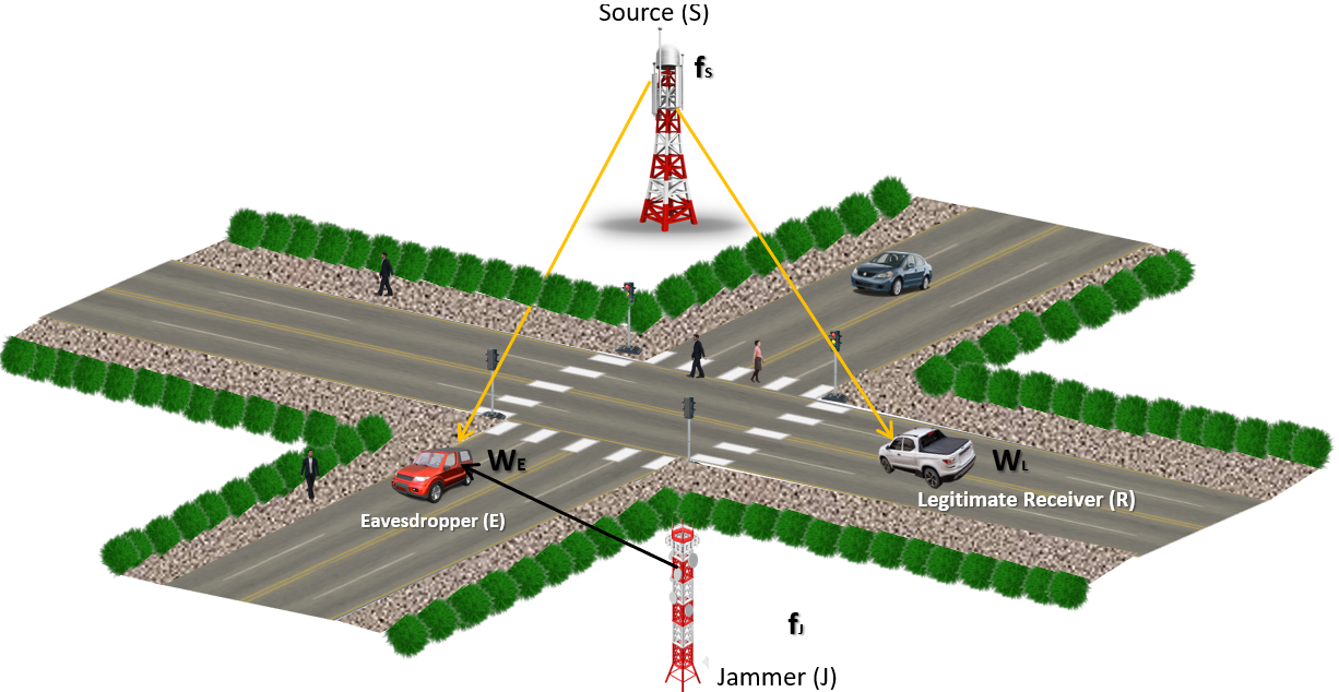
The communication model in Fig. 1 presents a typical model where the attacker E is overhearing the communication between the base station (BS) noted by and the legitimate receiver . To jam the signal received by the eavesdropper, we intend to employ a jammer , where its main goal is perturbing and minimizing the SINR at the attacker’s end.
We note that and are equipped with antennas, and both the legitimate receiver and the attacker are equipped with antennas.
II-B Channel Model
In this paper, we assume a Sub-6 GHz/mmWave system. Therefore, the channels follow a geometric model based on clusters and rays:
| (1) |
where and are, respectively, the number of clusters, the number of rays, the number of antennas at the receiver, and antennas at the transmitter. is the complex gain of the cluster and the . ray. The array steering and response vectors at the receiver (R) and the transmitter (T) are and , respectively. The angles of departure (DoD) and the angles of arrival (AoA) are denoted by and , respectively
The received signal at L and E are respectively:
| (2) |
| (3) |
where is the combiner vector at the node with dimension (). , and are respectively, the channel matrix from to , to , to , and to with dimensions . The precoders applied at and are defined by and with dimension . is the information symbol sent by transmitter where . Finally, is the zero mean additive white Gaussian noise (AWGN) with variance .
The received SNR and SINR at and , respectively, are
| (4) | ||||
| (5) | ||||
To improve the security performance of our communications model, we need to maximize the average secrecy capacity , which is defined as follows
| (6) |
where and are respectively the ergodic capacities at and and they are defined by
| (7) |
| (8) |
III Adaptive Gradient Ascent Algorithm
III-A Gradient Learning Approach Without Optimizing
Our goal is to maximize the secrecy capacity by searching for the adequate values of , and . Therefore, we are going to maximize the cost function in Eq. (6) under two constraints: the unit-norm and the CA constraints. We can formulate the optimization problem as follows
| (9) |
| (10) |
| (11) |
where Eq. (10) is the unit-norm constraint and Eq. (11) is the CA constraint ( and are the subspace of the CA constraints of dimensions and , respectively)[7]. We need to compute the gradients with respect to , and , then project the solutions onto the subspace of the CA constraints. Therefore, we will start by differentiating the cost function for , which is expressed as follow
| (12) | ||||
where and .
As a second step, we compute the gradient of , which is given by
| (13) |
where
| (14) |
| (15) |
where and .
| (16) |
Therefore, the gradient of is expressed by Eq. (16) on the top of the next page. Finally, we derive the gradient of as follow
| (17) |
Hence, we can first compute the partial derivative of the rate at the legitimate receiver node:
| (18) |
Then, we derive the partial derivative of the rate at the eavesdropper end:
| (19) |
Thereby, we can express the gradient of by:
| (20) |
After computing the gradients, we can now move to the Gradient ascent algorithm. We presents two different algorithms. Algorithm 1 search how to maximize the secrecy capacity while maintaining the source power fixed. This is very efficient in case where the power is limited. Hence, the algorithm search for the perfect precoders/combiners configuration that will maximize the secrecy under power constraints. On the other hand, Algorithm 2 search for the best precoders/combiners combinations but with respect to a secrecy capacity target required by the QoS. In this second approach, we fix and we search for the maximum possible secrecy capacity. If we achieve , the algorithm stops, otherwise it adapts while the power cannot exceed a certain threshold (to avoid infinite loop and unrealistic power consumption).
Adaptive Gradient Ascent for fixed transmission power ()
Adaptive Gradient Ascent for variable transmission power ()
III-B Gradient Learning Approach While Optimizing
To characterize the system performance, we used two different benchmarkers. The first one is computing the gradient of . It is clear that it is not feasible to design the combiner of the attacker. However, we can optimize with respect to , which of course will provide higher secrecy capacity, and we use the output result as a benchmarking tool. The gradient of , which is given by
| (21) | ||||
After computing , we optimize with respect to by implementing the following code line after the line with index in Algorithm 1:
III-C SVD Upper Bound
The second benchmarker is an upper bound by applying the singular value decomposition (SVD) on the channels , , , and . Therefore, the upper bound of the achievable rate is expressed as follow
| (22) | ||||
where , and are the maximum singular values of , and , respectively. and are the minimum singular value of and , respectively. Although, the rate (22) is not achievable, it is a tool to verify the optimized system performances.
IV Numerical Results and Discussions
| Parameters | mmWave | Sub-6 GHz |
| Number of antennas at the jammer | 64 | 16 |
| Number of antennas at the BS | 64 | 16 |
| Number of antennas at the receivers | 4 | 4 |
| Number of clusters | 4 | 10 |
| Number of rays per cluster | 15 | 20 |
| Angular spread | ||
| Power at the BS | 10 dB | 10 dB |
| Power at the BS | 10 dB | 10 dB |
| Step size | 0.1 | 0.1 |
| Convergence criterion | ||
| Power adaptation rate | ||
| Number of Monte Carlo simulation loops | 1000 | 1000 |
In this section, we will examine the performance of the proposed security scheme. To guarantee the convergence stability and to adjust any possible perturbation during the learning process, the step size parameter is initialized to 0.1 and it is divided by 2 whenever a perturbation occurs during the optimization cycle of the cost function. optimization. The channel matrices , , , the combiners , and the precoders , and are assumed to follow complex Gaussian distribution.

In Fig. 2, we studied the convergence rate of the optimization process for Sub-6 GHz and mmWave scenarios. We observe that the secrecy capacity for both scenarios converges with the same number of iterations which is 400 iterations. Regarding the achievable secrecy capacity (without optimizing ), Sub-6 GHz provides higher secrecy than the mmWave for the first 60 iterations. However, when the cost function starts to converge, mmWave offers 2.4 bps/Hz while Sub-6 GHz achieves about 2.1 bps/Hz. For the first benchmarker ( (while optimizing ), , and ), we observe that this upper bound and the curve related to the case of random are very close for the first 100 iterations and a gap starts to grow when the learning process starts to converge. We should note that the converged secrecy capacity did not exceed neither the first benchmarker, neither the second benchmarker( the SVD ceil) during the entire learning process.
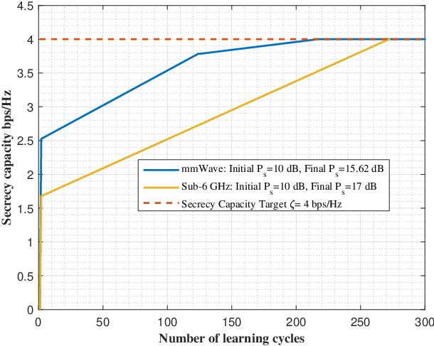
For the previous Fig. 2, we discussed the results of Algorithm 1, where is fixed. Now, we move to analyze Algorithm 2 by discussing Fig. 3. In this scenario, the source power from the BS is considered to be variable. Our goal is to achieve a secrecy capacity noted by . The algorithm searches for the maximum possible for a given , if the obtained value reaches , the learning process will stop, if not, the source power will be adapted and another learning cycle will initiate (where a cycle is referring to the learning process for a given ). In Fig. 3, the target secrecy capacity is =4 bps/Hz while starts at 10 dB. The algorithm arrives at the required after 212 cycles for mmWave system, while it spends 272 cycles for Sub-6 GHz. Regarding the source power needed to optain , at the end of the entire learning process, increased from 10 dB to 15.62 dB for Sub-6 GHz while it requires only 17 dB in the case of mmWave. Therefore, under the condition of secrecy capacity requirement, we observe that the learning rate (number of cycles required to reach ) for mmWave system case is much higher than the Sub-6 GHz, while there is no significant difference concerning the needed source power
V Conclusion
In this work, we discussed the PLS for V2I communication under the scenario of eavesdropping attack for two different cases: Sub-6 GHz and mmWave systems. We assumed the deployment of a friendly jammer that aids to maximize the average secrecy capacity. We used adaptive Gradient ascent as a machine learning approach to maximize the secrecy capacity while searching for the best combination of combiner at the legitimate receiver and precoders at BS/jammer. We proposed two different algorithms. In the first one, we assumed that the source power is fixed and we searched for the best precoders and combiner that maximize the secrecy capacity. We noted that the cost function converges to the maximum secrecy capacity with the same rate for both the Sub-6 GHz and mmWave systems where the later achieved higher secrecy capacity than the former. In the second algorithm, we suppose that the QoS requires a specific secrecy capacity threshold that we need to achieve while using the optimum source power. The mmWave system reached the secrecy target faster than the Sub-6 GHz.
References
- [1] S. K. Tayyaba, H. A. Khattak, A. Almogren, M. A. Shah, I. U. Din, I. Alkhalifa, and M. Guizani, “5g vehicular network resource management for improving radio access through machine learning,” IEEE Access, vol. 8, pp. 6792–6800, 2020.
- [2] Y. Yang, Z. Gao, Y. Ma, B. Cao, and D. He, “Machine learning enabling analog beam selection for concurrent transmissions in millimeter-wave v2v communications,” IEEE Transactions on Vehicular Technology, vol. 69, no. 8, pp. 9185–9189, 2020.
- [3] M. Arif, G. Wang, M. Z. A. Bhuiyan, T. Wang, and J. Chen, “A survey on security attacks in vanets: Communication, applications and challenges,” Vehicular Communications, vol. 19, p. 100179, 2019.
- [4] Deeksha, A. Kumar, and M. Bansal, “A review on vanet security attacks and their countermeasure,” in 2017 4th International Conference on Signal Processing, Computing and Control (ISPCC), 2017, pp. 580–585.
- [5] Y. Ai, M. Cheffena, A. Mathur, and H. Lei, “On physical layer security of double rayleigh fading channels for vehicular communications,” IEEE Wireless Communications Letters, vol. 7, no. 6, pp. 1038–1041, 2018.
- [6] N. Mensi, D. B. Rawat, and E. Balti, “PLS for V2I Communications Using Friendly Jammer and Double kappa-mu Shadowed Fading,” in 2021 IEEE International Conference on Communications (IEEE ICC’21), Montreal, Canada, Jun. 2021.
- [7] E. Balti and N. Mensi, “Zero-forcing max-power beamforming for hybrid mmwave full-duplex mimo systems,” in 2020 4th International Conference on Advanced Systems and Emergent Technologies (IC_ASET), 2020, pp. 344–349.