A Measurement of Stellar Surface Gravity Hidden in Radial Velocity Differences of Co-moving Stars
Abstract
The gravitational redshift induced by stellar surface gravity is notoriously difficult to measure for non-degenerate stars, since its amplitude is small in comparison with the typical Doppler shift induced by stellar radial velocity. In this study, we make use of the large observational data set of the Gaia mission to achieve a significant reduction of noise caused by these random stellar motions. By measuring the differences in velocities between the components of pairs of co-moving stars and wide binaries, we are able to statistically measure the combined effects of gravitational redshift and convective blueshifting of spectral lines, and nullify the effect of the peculiar motions of the stars. For the subset of stars considered in this study, we find a positive correlation between the observed differences in Gaia radial velocities and the differences in surface gravity and convective blueshift inferred from effective temperature and luminosity measurements. The results rule out a null signal at the level for our full data-set. Additionally, we study the sub-dominant effects of binary motion, and possible systematic errors in radial velocity measurements within Gaia. Results from the technique presented in this study are expected to improve significantly with data from the next Gaia data release. Such improvements could be used to constrain the mass-luminosity relation and stellar models which predict the magnitude of convective blueshift.
Keywords:
astrometry, gravitation, (stars:) binaries: general, convectionI Introduction
The advent of the Gaia space telescope has given rise to a new era of precision astrometry with a current catalog that includes over one billion stars, of which several millions have radial velocity (RV) measurements. Such a large data set offers new opportunities to statistically measure stellar properties. In this study, we use RV measurements from Gaia to measure the gravitational redshift (GR) due to stellar surface gravity (SG), as well as the subdominant effect of convective outflows and downflows at the stellar surface.
Understanding these effects is important since they give rise to systematic noise in RV measurements, and in particular raise difficulties in RV detection of exoplanets (see e.g. Wright 2018, for a review). Additionally, measurement of convective effects could shed light on physical processes occurring within stars and constrain current and future modeling of these processes.


The Gaia mission performs RV measurements by measuring the Doppler shift of a few common absorption lines using the Radial Velocity Spectrometer (RVS). Although the frequency shift observed by the RVS is reported as a relative velocity between the emitting star and the Gaia satellite, there are many additional effects that can contribute (see e.g., Lindegren & Dravins 2003, for an overview). In particular, the SG of the emitting star results in a redshift of line frequencies measured by the RVS, biasing RV measurements to be slightly more positive than their true values. While the true velocities are typically on the order of the galactic virial velocity, km/sec, typical values from GR are,
| (1) |
Thus, GR in non-degenerate stars is usually a small contribution to the RV.
An additional effect on RV measurements arises from convective motion on the stellar surface. Hot and luminous outflows typically result in a net blueshift of emitted photons and measured RVs appear, on average, smaller (more negative) than their true values. This effect is known as convective blueshift (CB). The size of the effect depends on stellar type and can induce effective RV measurements of order, , and hence is generally subdominant to GR.
Although existing spectrometers have the necessary precision to observe GR, this measurement is challenging since the true velocity of any particular star is unknown, contributing a statistical uncertainty on the order of . This difficulty has been overcome in only a few types of systems. Original measurements of GR were performed on white dwarfs in binary systems, most notably the nearby Sirius B (Greenstein et al. 1971). These can have GRs as large as (Greenstein & Trimble 1967), making detection relatively straightforward. Additionally, there have been long-standing efforts to extract the GR of the Sun, which is expected to be (Lindegren & Dravins 2003). This is challenged by a CB of comparable size, which itself depends sensitively on the spectral line and its angular position. A recent clean measurement and some discussion of its history can be found in González Hernández et al. 2020.
The difficulty of disentangling GR from physical motion in stars can be reduced with statistics of large data sets and an appropriate choice of stellar system. A previous attempt to statistically measure GR in ordinary stars was performed using the M67 open clusters in Pasquini et al. 2011. However, that study was unable to extract a signal above the background, which the authors hypothesized as due to unsubtracted CB effects. More recently, Leão et al. 2019 compared spectroscopic and astrometric RVs for stars in the Hyades open cluster. That study was able to measure the combined effects of GR and CB, however their data sample was small and included only two giants. Finally Dai et al. 2019 attempted a measurement of stellar GR by averaging Gaia RV measurements over stars of different types. Their results show some evidence for a combination of GR and CB and they did not attempt to distinguish between or characterize the different contributions.
In this study, we search for GR in co-moving pairs of stars, thousands of which have been identified in Gaia DR2. If these co-moving pairs are wide binaries, their orbital velocities should be small, providing a clean data set with which to study small contributions to RVs. In particular, the difference of the RVs of two stars in a wide binary can be dominated by the difference in , especially for pairs of stars with sizeable differences in mass and/or radius. This opens the possibility of using wide binaries to directly probe GR and indirectly gain information regarding stellar structure and dynamics.
The main results of this study are presented in Fig. 1, which shows the correlation between the differences of the observed RVs of stars in co-moving pairs and the expectation from GR and CB. The left panel corresponds to a data set with higher statistics but also high uncertainty on stellar mass, while the right panel corresponds to a smaller sample with high quality mass measurements. A positive correlation is observed, corresponding to an agreement between model and data within measurement errors, with a non-zero slope at the level.
The study is structured as follows. First, we present details of the data selection used for this study. We follow with a discussion of GR- and CB-induced changes in measured RVs. Next, we present our analysis technique and discuss the dispersion observed in the data, concluding with a discussion of our main results, possible issues, and future prospects.
II Data Selection
Comoving pairs in physical (3-dimensional) velocity were first compiled using Gaia DR1 by Oh et al. 2017. Such stars are typically wide binaries with separation distances Allen et al. 2000, and are distinct from typical binaries in that they are likely to have been born at the same time and share a similar chemical composition. This has led to considerable interest in compiling lists of wide binaries with 3741 pairs identified in DR2 Jiménez-Esteban et al. 2019, and statistical analyses performed by Zavada & Píška 2018. Additionally, Hartman & Lepine 2020 created the SUPERWIDE catalog of wide binaries. This catalog is selected from Gaia DR2 and the SUPERBLINK high proper motion catalog (Lépine 2005; Lépine & Gaidos 2011). Importantly, selection of these wide binary pairs is completely independent of RV measurements.
We analyze the subset of SUPERWIDE pairs that also have RV measurements in Gaia DR2. Additionally, we require that the difference in the RVs of each star in a pair, , has a small measurement error, , and we remove outlier pairs with . To reduce contamination from the orbital velocities of wide binaries, we require that the transverse separation of the stars in a pair, , be greater than . Finally, we require that all stars have estimated values for effective temperature, , luminosity, , and radius, , from Gaia DR2. A total of 1,682 pairs pass these selection criteria.
Since we are interested in estimating the masses and radii of stars in our data set with high accuracy, it is beneficial to categorize stars as either main sequence (MS) stars or as giants. The selection criteria used in this study are marked in red in Fig. 2. MS stars are defined to lie within the solid curves.11 1 These curves are a multiplicative factor of from an curve which corresponds to the luminosity at which the highest number density is obtained across all stars in Gaia DR2 that pass the selection criteria suggested in Gaia Collaboration et al. 2018. The curve is restricted to and to ensure that the mass-luminosity relation from Malkov 2007 is valid. These criteria also assist in excluding wide binaries that are in fact triple systems containing an unresolved inner binary, which otherwise might contaminate the sample. Giants are defined to lie above the dashed curve, which corresponds to . A total of 1,135 pairs pass these additional selection criteria in our primary data set, of which 1,080 contain two MS stars, 53 contain one MS star and one giant, and 2 contain two giant stars.
We estimate the masses of MS stars using the mass-luminosity relation,
| (2) |
where , , and (Malkov 2007). However, we note that there is considerable uncertainty on the precise form of this relation. We conservatively assume an uncertainty of in the masses estimated using Eq. (2).

For giant stars, the stellar mass can in principle be inferred directly from photometric observations via asteroseismology. However, this requires long photometric observation times and cannot be done with Gaia photometry. In order to preserve a sizeable statistical sample of giants, we uniformly set the masses of all selected giants to the average asteroseismologically determined mass from the Kepler mission, (Yu et al. 2018). We estimate the uncertainty on the fixed giant mass to be . This ad hoc estimation of the giant masses has a negligible effect on the GR signal in a MS - giant comoving pair, since the radius selection cut of ensures that the GR contribution from giants is of that from MS stars.
In addition to the primary data set discussed above, we also identify a distinct set of comoving pairs for which both stars have high quality spectroscopic mass and radius measurements from Sanders & Das 2018. Stars from this set of 114 pairs are marked in blue in Fig. 2. In principle, some of these star’s RVs could also be measured directly from their spectra instead of the Gaia RVS, however we do not consider this possibility in the current study since the small statistics of the secondary data set is extremely limiting anyway.
To test consistency between the data sets, Fig. 3 shows a comparison of values of SG, g, between the data sets, as reported by Gaia and Sanders & Das 2018. Specifically, for all star that are in both data sets, we plot a histogram of the differences in SG normalized to the spectroscopic value. We find that the differences in measurements of SG between the primary and secondary data set are of order or less. Tables of additional properties of stars in each pair of both data sets is available in the online Supplemental Material of this study through the journal webpage.
With these two data sets at hand, we proceed to estimate the effects of differences in GR and CB between stars in each pair.
III Gravitational Redshift
The difference in measured RV between two stars (labelled 1 and 2), induced by GR alone, is given by
| (3) |
Since giants have considerably larger radii, they tend to contribute negligibly to GR. Additionally, the GR of two MS stars tends to partially cancel. Thus, the largest signal comes from MS - giant pairs.
The masses and radii in Eq. (3) are estimated as described above (depending on the data set being used). For each co-moving pair, a distinct value of can be calculated and compared to the measured RV of the pair. This comparison is complicated by the presence of sub-dominant effects such as CB.
IV Convective Blueshift
The surface of a star is characterized by the presence of convective cells where hot gas rises outwards, and cooler gas sinks through intergranular lanes. Since the hotter rising gas is brighter than the cooler sinking gas, a net blueshift is produced in the disk-integrated light emitted by the star. This phenomenon is usually referred to as CB (Beckers & Nelson 1978; Dravins 1982, e.g.).
Since CB depends on complex details of turbulent convection, it is notoriously difficult to predict. This presents a major challenge in, for example, exoplanet searches looking for modulations in spectral lines due to planetary motion around distant stars (see e.g. Wright 2018, for a review). Attempts to estimate the amplitude of this effect for different stellar types rely on hydrodynamic simulations of surface convection. Such calculations were performed in Allende Prieto et al. 2013 for typical stellar types in the Gaia catalog, finding amplitudes of CBs in the range , depending on the mass and temperature of the star. While magneto-hydrodynamic calculations might provide a more complete picture, recent measurements show that magnetic activity is only mildly correlated with CB (Meunier, N. et al. 2017; Meunier et al. 2017).
To parametrize the effect of CB we define the difference between stars 1 and 2 as (note that are typically negative) and apply the theoretical fitting formula provided in Allende Prieto et al. 2013. This fit requires estimates of both metallicity and SG, which are not reported in Gaia spectroscopic data. For our primary data set, we estimate metallicity using the Gaia RV template metallicity, and SG using the mass and radius estimates described above. For our secondary data set, we use metallicity and SG measurements reported in Sanders & Das 2018. Although the dependence of CB on metallicity is relatively weak, is highly sensitive to SG. Therefore, the use of Eq. (2) may introduce sizeable errors in for the primary data set.
V Analysis
For each pair in our data sets we calculate according to Eq. (3) and using the fitting formula of Allende Prieto et al. 2013. For stars in our primary data set, we estimate stellar masses and radii as described above; for our secondary data set we use the mass and radius estimates provided in Sanders & Das 2018.
In the absence of background effects, one expects RV to be directly correlated with . This relationship is shown in Fig. 1. The left panel corresponds to the primary data set, for which the lack of high quality mass estimates introduces large errors in and . The right panel corresponds to the secondary data set for which is more precise but statistics are much lower. Grey points represent the pairs in each data set along with their corresponding uncertainties. The ordering of stars in each pair is chosen such that the value on the horizontal axis is positive. Orange points correspond to the average value of RV in bins of , and are shown for illustrative purposes only.
In each case we test how well the model (horizontal axis, denoted ) fits the data (vertical axis, denoted ). If all background effects averaged to zero, one would expect a linear fit of the form with and . We find that this linear model is a poor fit to both data sets, mainly due to a dispersion of the measured RV values which is larger than that expected from measurement errors alone. That is, we find that there is an intrinsic source of dispersion in our RV measurements. We discuss possible sources of this dispersion below and account for it by introducing an additional model parameter, . We then analyze the data using the Gaussian likelihood,
| (4) |
where is the effective uncertainty of each data point, and the index runs over all pairs in a given data set. This likelihood is maximized and used to compute confidence intervals for the slope parameter , with the dispersion treated as a nuisance parameter. The dashed black lines in Fig. 1 represent the function , where is the maximum likelihood value of the corresponding data set, and the blue bands correspond to the 1 (68%) confidence interval around this slope. For our primary (secondary) data set, we find that the maximum-likelihood excess dispersion is () km/sec.
VI Excess Dispersion of the Data
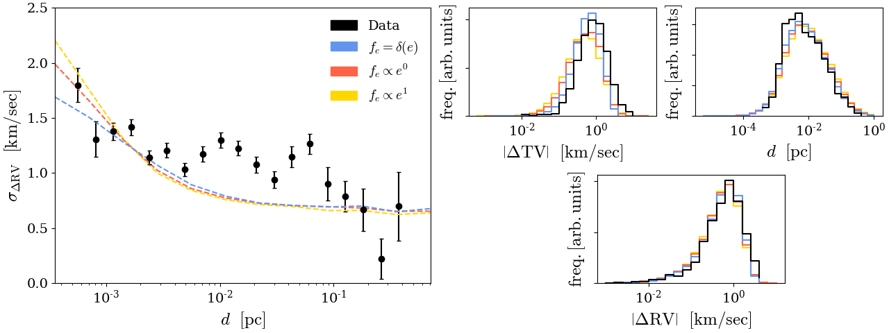
Radial orbital motions of binary systems should contribute a dispersion to RV measurements and could be the source of . To check this assumption, we have performed a Monte Carlo (MC) analysis by simulating binary systems with random orientations, including the effects of RV measurement errors in Gaia. The mass distribution of stars within the simulation and RV measurement errors are taken from the data. The distribution of semi-major axes is estimated by performing a de-convolution (Lucy 1974) of the projected 2D separation of stars, , as measured in the data, under the approximation of circular orbits for all binaries. The distribution of eccentricities is modeled either as a power law (Moe & Di Stefano 2017), such that the distribution scales as with or , or taken to be zero for all binaries (circular orbits).
The left panel of Fig. 4 shows the dispersion of measured RV as a function of for the primary data set, compared with the MC results. The MC curves are dominated by binary motion at small values of and by RV measurement errors at large . The data is a good fit to the MC curve, except at intermediate values of pc, hinting that binary motion is a significant source of excess dispersion at small separations. However, since the MC underestimates the dispersion at intermediate separations, there is likely an unidentified additional contribution.
One possibility is that the RV errors quoted in the Gaia catalog are underestimated. The excess dispersion found in this study can be explained if there are experimental uncertainties of present in Gaia RVS measurements.
VII Discussion
| systematic checks | slope |
|---|---|
| primary | |
| narrow main sequence | |
| observational main sequence | |
| km/sec | |
| km/sec | |
The main results of this study are summarized in Fig. 1. We find a significant correlation between RV and , corresponding to a linear fit of the form , with a slope of order unity. Specifically, for both data sets considered in this study, the best fit slope is consistent with to within measurement errors and inconsistent with zero at the () level for the primary (secondary) data set. In the secondary data set, even though the data is more precise, there is a large error in due to low statistics.
In addition to the results shown in Fig. 1, we have performed our analysis with slight variations to the data selection and parameter estimation described above. Details of these variations and the resulting values for are summarized in Table 1. We find that these modifications do not qualitatively change our results.
We find an excess dispersion in the data of order km/sec that is likely dominated by binary motion at small separations, with some unknown contribution at intermediate separations. A possible explanation is that RV errors in Gaia are underestimated, however we are unable to pinpoint the origin of the excess dispersion with a high level of certainty.
Moreover, we note that Gaia RVS measurements may exhibit a systematic bias toward high RVs for dim stars (Katz et al. 2019) with corrections up to for apparent magnitudes of , and negligible bias for stars brighter than . Our primary (secondary) data set exhibits stars with a mean value of and standard deviation of . Since apparent magnitude is correlated with stellar SG, such a systematic bias would serve to enhance, or possibly mimic a GR signal, and might explain the fact that we consistently find in the analysis. Correcting for this bias, if it exists, is challenging due to the large uncertainty in the size of the effect. We do not attempt a detailed study, but note that taking the bias to vanish for and linearly increasing for , with a slope of , reduces the slope in the left panel of Fig. 1 to . One potential discriminator between such a systematic error and a GR signal is that a dependence on need not manifest as a linear relation in Fig. 1 (due primarily to the non-trivial relation between apparent magnitude and SG). With future data, one could robustly test if this effect is substantial.
Systematic uncertainties in the determination of the stellar parameters could also have an impact on our results. For example, a systematic shift in the derived effective temperatures due to unknown reddening would result in different CB corrections than those discussed in Sec. IV. Additionally, CB predictions rely on 3D simulations which are uncertain. Calibration of these models using solar observations revealed discrepancies up to 0.2 km/sec between predictions and observations that may be due to NLTE effects (González Hernández et al. 2020). However, it is difficult to estimate this source of uncertainty in the full regime of stellar parameters discussed in this work.
In principle, modifications of the technique developed in this study could be used to test relations such as Eq. (2) and the fitting formula provided in Allende Prieto et al. 2013. Ultimately, this would be a novel probe of stellar structure and could, for example, assist in an improved understanding of systematics currently prohibiting better measurements of exoplanets and their properties. With the current data, low statistics limit a meaningful test of such models; however, the next Gaia data release (DR3) is expected to include many more stars with RV measurements and may allow for such an analysis to be performed. In the current study we have shown that a significant signal can be extracted from Gaia data.
VIII Data Availability
The data underlying this article are available in the article and in its online supplementary material.
Acknowledgments
We thank David Hogg for advice and guidance in the early stages of this study. We also thank David Spergel, Jason Hunt, and George Seabroke for useful conversations. JD was supported in part by the DOE under contract DE-AC02-05CH11231 and in part by the NSF CAREER grant PHY-1915852. OS was supported by the DOE under Award Number DE-SC0007968 and the Binational Science Foundation (grant No. 2018140).
References
- Allen et al. (2000) Allen, C., Poveda, A., & Herrera, M. A. 2000, A&A, 356, 529
- Allende Prieto et al. (2013) Allende Prieto, C., Koesterke, L., Ludwig, H. G., Freytag, B., & Caffau, E. 2013, A&A, 550, A103, doi: 10.1051/0004-6361/201220064
- Beckers & Nelson (1978) Beckers, J. M., & Nelson, G. D. 1978, Sol. Phys., 58, 243, doi: 10.1007/BF00157270
- Dai et al. (2019) Dai, D.-C., Li, Z., & Stojkovic, D. 2019, Astrophys. J., 871, 119, doi: 10.3847/1538-4357/aaf6aa
- Dravins (1982) Dravins, D. 1982, ARA&A, 20, 61, doi: 10.1146/annurev.aa.20.090182.000425
- Gaia Collaboration et al. (2018) Gaia Collaboration, Babusiaux, C., van Leeuwen, F., et al. 2018, A&A, 616, A10, doi: 10.1051/0004-6361/201832843
- González Hernández et al. (2020) González Hernández, J., et al. 2020, Astron. Astrophys., 643, A146, doi: 10.1051/0004-6361/202038937
- González Hernández et al. (2020) González Hernández, J. I., Rebolo, R., Pasquini, L., et al. 2020, A&A, 643, A146, doi: 10.1051/0004-6361/202038937
- Greenstein et al. (1971) Greenstein, J. L., Oke, J. B., & Shipman, H. L. 1971, ApJ, 169, 563, doi: 10.1086/151174
- Greenstein & Trimble (1967) Greenstein, J. L., & Trimble, V. L. 1967, Astrophysical Journal, 149, 283, doi: 10.1086/149254
- Hartman & Lepine (2020) Hartman, Z. D., & Lepine, S. 2020, The Astrophysical Journal Supplement Series, 247, 66, doi: 10.3847/1538-4365/ab79a6
- Jiménez-Esteban et al. (2019) Jiménez-Esteban, F. M., Solano, E., & Rodrigo, C. 2019, AJ, 157, 78, doi: 10.3847/1538-3881/aafacc
- Katz et al. (2019) Katz, D., Sartoretti, P., Cropper, M., et al. 2019, A&A, 622, A205, doi: 10.1051/0004-6361/201833273
- Leão et al. (2019) Leão, I. C., Pasquini, L., Ludwig, H. G., & de Medeiros, J. R. 2019, MNRAS, 483, 5026, doi: 10.1093/mnras/sty3215
- Lépine (2005) Lépine, S. 2005, AJ, 130, 1247, doi: 10.1086/432161
- Lépine & Gaidos (2011) Lépine, S., & Gaidos, E. 2011, AJ, 142, 138, doi: 10.1088/0004-6256/142/4/138
- Lindegren & Dravins (2003) Lindegren, L., & Dravins, D. 2003, Astron. Astrophys., 401, 1185, doi: 10.1051/0004-6361:20030181
- Lucy (1974) Lucy, L. B. 1974, AJ, 79, 745, doi: 10.1086/111605
- Malkov (2007) Malkov, O. Y. 2007, Monthly Notices of the Royal Astronomical Society, 382, 1073, doi: 10.1111/j.1365-2966.2007.12086.x
- Meunier et al. (2017) Meunier, N., Lagrange, A. M., Mbemba Kabuiku, L., et al. 2017, Astronomy & Astrophysics, 597, A52, doi: 10.1051/0004-6361/201629052
- Meunier, N. et al. (2017) Meunier, N., Lagrange, A.-M., Mbemba Kabuiku, L., et al. 2017, Astronomy & Astrophysics, 597, A52, doi: 10.1051/0004-6361/201629052
- Moe & Di Stefano (2017) Moe, M., & Di Stefano, R. 2017, ApJS, 230, 15, doi: 10.3847/1538-4365/aa6fb6
- Oh et al. (2017) Oh, S., Price-Whelan, A. M., Hogg, D. W., Morton, T. D., & Spergel, D. N. 2017, The Astronomical Journal, 153, 257, doi: 10.3847/1538-3881/aa6ffd
- Pasquini et al. (2011) Pasquini, L., Melo, C., Chavero, C., et al. 2011, A&A, 526, A127, doi: 10.1051/0004-6361/201015337
- Sanders & Das (2018) Sanders, J. L., & Das, P. 2018, MNRAS, 481, 4093, doi: 10.1093/mnras/sty2490
- Wright (2018) Wright, J. T. 2018, Radial Velocities as an Exoplanet Discovery Method, 4, doi: 10.1007/978-3-319-55333-7_4
- Yu et al. (2018) Yu, J., Huber, D., Bedding, T. R., et al. 2018, The Astrophysical Journal Supplement Series, 236, 42, doi: 10.3847/1538-4365/aaaf74
- Zavada & Píška (2018) Zavada, P., & Píška, K. 2018, arXiv e-prints, arXiv:1810.13270. https://arxiv.org/abs/1810.13270