Integration of activation maps of epicardial veins in computational cardiac electrophysiologyJournal: Computers in Biology and Medicine
Abstract
In this work we address the issue of validating the monodomain equation used in combination with the Bueno-Orovio ionic model for the prediction of the activation times in cardiac electro-physiology of the left ventricle. To this aim, we consider four patients who suffered from Left Bundle Branch Block (LBBB). We use activation maps performed at the septum as input data for the model and maps at the epicardial veins for the validation. In particular, a first set (half) of the latter are used to estimate the conductivities of the patient and a second set (the remaining half) to compute the errors of the numerical simulations. We find an excellent agreement between measures and numerical results. Our validated computational tool could be used to accurately predict activation times at the epicardial veins with a short mapping, i.e. by using only a part (the most proximal) of the standard acquisition points, thus reducing the invasive procedure and exposure to radiation.
Keywords:
Cardiac electro-physiology, monodomain equation, Bueno-Orovio ionic model, activation times, Ensite Precision system, Cardiac Resynchronization Therapy1 Introduction
Electrophysiology is a fundamental research field in applied mathematics since Hodgkin and Huxley described for the first time the propagation of action potentials in cells [5]. Mathematical and numerical modeling in cardiac electrophysiology in the last decades have assumed a key role to better understand cardiac muscle function and to study how several cardiac diseases develop and to provide concrete answers to clinical problems. Challenging issues consist of selecting accurate and efficient numerical methods for the approximate solution of such models and in the estimation of the model parameters to fit patient-specific data.
To describe the propagation of the electrical signal in the heart muscle two possible mathematical approaches are the bidomain and the monodomain models [55, 54]. The former is the result of the application of conservation of charge together with constitutive models. It describes the propagation of the trans-membrane potential and compute both the internal and external cell potentials. The monodomain model is a simplification of the bidomain one, assuming that the external and internal conductivity tensors are proportional. Both models have to be coupled with a ionic model, a system of ODEs which describes the evolution of the trans-membrane potential in a single cell by means of suitable gating variables.
Validation of these mathematical models, i.e. the certification that a model could be used for predictive purposes, is fundamental to provide clinicians a reliable tool to study and predict the cardiac function accurately.
A first attempt in this direction consisted of comparing numerical results (obtained either by the bidomain or monodomain model) with measures of electrical activity obtained by optical imaging during ex-vivo experiments on animal hearts. In particular, qualitative comparisons have been provided in [44, 65] for action potentials and in [59, 19] for activation times. Other works instead quantified the discrepancy between results and measures; in particular in [6, 1] the authors focused on the action potential, whereas in [49, 31, 40] on activation times. In [7], the authors considered a similar calibration of the monodomain model by using data of activation times acquired by catheters in pigs.
A second set of results focused on human ideal geometries, proposing benchmark simulation protocols to be validated against gold-standard activation times obtained from experimental measures. In particular, [67] considered a slab of tissue, whereas [68] an idealized left ventricle.
Another group of studies addressed qualitative comparisons in real human geometries. In particular, in [35] the authors compared the phase distribution during ventricular fibrillation with some reference electrical data, whereas in [16] they studied the reliability of ECG obtained with an electro-mechanical simulation. Instead, in [24], the authors performed a calibration of the monodomain model on human data by using a probabilistic model (Bayesian influence method).
Other works have considered the inclusion of electrical data of human activation time obtained by catheter in a computational framework to calibrate the conduction properties of the tissue [52, 27, 50, 45, 15, 69, 13, 8]. For example, in [15, 69] a quantitative comparison between in-vivo measures of activation times acquired at the endocardium and those provided by the Eikonal equation in the presence of a personalized Purkinje network was carried out. Instead, in [10] the authors validated the monodomain model with a Mitchell-Schaeffer ionic model in the left atrium under the S1 and S2 stimulation protocols. Among the previous studies, only [8] considered measures at the ventricular epicardial veins. In particular, the reaction-Eikonal equation was used to find the most accurate model among six electrophysiology surrogate models able to reproduce the electrical activation during right ventricle apex stimulation.
Of previous cited works, the majority conducted a calibration of the model considered for their study, i.e. all the data at disposal have been used to estimate some conductivity parameters to match the data. Instead, only few works used different sets of data (in some cases also of different nature) to calibrate the model and to assess the error against clinical measures (with a little abuse of terminology, we refer to this as cross-validation, as done in statistics when the results obtained from the statistical analysis are compared with the testing data selected randomly and not used in the calibration). In particular, the two sets are given by action potential data in pigs at different stimulation cycle lengths in [1], depolarization times and together with the blood pressure in [45], activation times at different locations in [15, 69] for the Eikonal model, ECG and epicardial activation times in [8] for the reaction-Eikonal model, atrial activation times for different stimulations in [10].
Our work aims at proposing an approach for validating the monodomain model in the context of the electrical propagation in the human left ventricle using patient-specific activation measures acquired at the epicardial veins. In particular, we only consider excitations with sinus rhythm, and not, tachicardia, fibrillation, and stimulated cases. Notice that, with sinus rhythm here we refer also to pathological cases (such as Left Bundle Branch Block (LBBB) without scar), provided that the front propagates without irregular or chaotic patterns. For each patient we had at disposal activation times at some points located at the septum and at the epicardial veins. The first dataset was used to provide a patient-specific input for the numerical simulation, whereas the second one was split into two subgroups, the first one used to estimate the conductivities of the patient and the second one to validate the accuracy of the numerical solution. Notice that the protocol of validation we described is quite general in the sense that the use of measurements acquired by means of catheters is not essential; in principle, comparison and minimization against activation maps acquired for example by electrode array recordings and optical mapping are possible. At the best of authors knowledge, this is the first cross-validation test for the monodomain model performed for the ventricular activation against clinical measures of activation times.
2 Methods
2.1 Mathematical and numerical model
In this section we present the mathematical model for cardiac electrophysiology, i.e. the monodomain model, and the corresponding numerical methods considered in this work. The choice of the monodomain model has been motivated by its lower computational cost, yet providing comparable accuracy, with respect to the bidomain model, at least in the cases of sinus rhythms [44].
Referring to Figure 1, the cardiac tissue conductivity is modeled as a tensor defined as
| (1) |
where , and are the conductivities along the fibers direction , the normal direction and the transversal direction (orthogonal to the sheets plane -), respectively, to be determined in order to fit the patient-specific activation times.

Assuming an external applied stimulus (provided in our case by activation time measures located at the septum, see below), the monodomain model in the computational domain and over a time interval reads [56, 4]:
Find, for each , the electrical potential and the gating variables , such that
| (2a) | |||||
| (2b) | |||||
where the ionic current and are chosen according to the Bueno-Orovio ionic model [2]. In particular, , with
| (3a) | ||||
| (3b) | ||||
| (3c) | ||||
for suitable constants and where is the Heaviside function. Moreover, is the surface area-to-volume ratio and the trans-membrane capacitance. System (2) has been equipped with suitable initial conditions for and and homogeneous Neumann conditions on for .
The time discretization we used to numerically approximate system (2) relies at each time step first on a forward Euler method for equation (2b), i.e.
| (4) |
being the time step length, and then on a first order semi-implicit method for (2a), i.e.
| (5) |
with
| (6) |
where the diffusion term has been treated implicitly and the non-linear terms have been linearized, see also [58]. In particular, at each time we first updated for a given by means of (4), then we solved (5) and (6) by using the up-to-date gating variables. Such time discretization lead to a conditionally stable method with a bound on time step which is independent of the mesh size and which is milder with respect to the required to reach the desired accuracy [47, 56].
As for the space discretization, we used continuous Finite Elements of order 1 (Q1) on hexahedral meshes. The ionic current term has been discretized using the Ionic Current Interpolation (ICI) method [66]: first has been computed using the values of and at the degrees of freedom, then it has been interpolated at quadrature nodes. Such approach is relatively inexpensive and less memory-demanding than solving the ODE system and computing directly at quadrature nodes (SVI), while the numerical accuracy is not affected at the small mesh size required to capture the propagating front. The resulting linear system arising at each time step has been solved by the GMRES method [72] preconditioned with the Jacobi preconditioner.
We have used a time step and a characteristic mesh size . Notice that both these values are small enough to recover an accurate propagation front [47, 70, 56, 30], see in particular [20] for the case of hexahedral meshes with Q1 Finite Elements, as in our case.
Finally, we highlight the importance of including cardiac fibers in electrophysiology models, since electrical propagation occurs in a different way along the fibers and orthogonally to them. Since standard imaging techniques do not provide geometric information on the fibers, whose dimension is typically smaller than the spatial resolution, the fiber orientation over the myocardial tissue has been here determined using the Laplace-Dirichlet rule-based algorithm described in [32]. In particular, we used a linear rule with the following boundary values for the fibers and the sheets angles: for fibers at the epicardium, for fibers at endocardium, for sheets on epicardium and for sheets on endocardium [32, 60].
The Laplace-Dirichlet rule-based fiber generation algorithm as well as all the numerical methods for the monodomain equation have been implemented within lifex
(https://lifex.gitlab.io/lifex), a new in-house developed high-performance C++ library mainly focused on cardiac applications, based on the deal.II Finite Element core [18];
for further details
on the implementation of the fibers generation see [61].
Electrophysiology simulations ran on 48 cores of a 192 cores node Platinum Intel® Xeon® 8160 @2.1GHz with 1.7TB RAM.
2.2 Processing of geometric and electrical data
In this section we illustrate the strategies used for data processing. In particular, in Section 2.2.1 we detail the geometric reconstruction, whereas in Section 2.2.2 the activation time maps and their integration with geometric data. Finally, in Section 2.2.3 we set the inverse problem used to provide the integration of electrical data into the numerical experiments and the estimation of the conductivities for a validation of the monodomain model in the context of a sinus rhythm. All the medical data, both geometric and electrical, have been provided by Ospedale S. Maria del Carmine, Rovereto (TN), Italy.
Four patients have been considered, from now on referred to as P1, P2, P3, and P4. They were all affected by a LBBB, a cardiac conduction abnormality due to an interruption of the electrical conduction in the His bundle which causes a delayed activation of the left ventricle. LBBB was diagnosed owing to ECG evaluation. In all patients scar regions were absent and the mapping procedure was performed by clinicians during the implantation of the Cardiac Resynchronization Therapy (CRT), in accordance with the standard clinical procedures.
All patients have been previously informed and gave their full consent for the acquisition of both the geometric and electrical data and for the successive mathematical analyses.
2.2.1 Imaging data acquisition and geometric reconstruction
The four subjects considered in the present study underwent a cineMRI steady-state free precession ECG/Retro with a 1.5-Tesla MRI Unit (Magnetom Aera, Siemens Medical Systems, Erlangen, Germany). The following parameters have been used: in-plane resolution and slice thickness ; TR (repetition time) ; TE (echo time) ; flip angle ; averages ; SNR (signal noise ratio) .
We performed a semi-automatic segmentation of the left ventricle geometry by using the free open-source software MITK [51], which allowed us to segment each MRI slice and to interpolate the ventricle surface between slices. In particular, for each patient MRI dataset, we have preliminary applied a manual correction of slice misalignment due to motion and breath artefacts. The next step of the segmentation procedure consisted of capping the two surfaces at the base of the ventricle, then to connect them with a triangulated base using the approach reported in [42]. Once two closed triangulated surfaces of both epicardium and endocardium of the left ventricle were obtained, a surface mesh was generated by means of a set of new meshing tools [42] developed as an extension to the VMTK software [37]. A remeshing procedure on the whole closed surface was then performed in order to prescribe a target mesh size. Finally, a volumetric hexahedral mesh of the left ventricle was generated. In Figure 2 the four patient-specific reconstructed volumes of the left ventricles with the generated muscle fibers are displayed.


2.2.2 Activation maps acquisition
A mapping of the septal surface located in the right ventricle and of the coronary veins located at the epicardium of the left ventricle has been performed (from 7 to 10 days after the MRI acquisition) for all the four subjects through the use of the Ensite Precision system [12] to record local activation times (referred to also as electrical data). The latter represent, for each point of acquisition, the time difference between two instants, one measured on an extracardiac reference electrode and another one representing the steepest negative intrinsic deflection in the electrogram recorded on an intracardiac electrode and indicating that the activation wavefront has reached the point under investigation. The Ensite Precision system allows to perform an accurate real-time three dimensional catheter navigation to obtain maps of activation times. For this study, a 5 Fr steerable 10-pole catheter has been inserted through the left subclavian vein. These data are available from multiple beats in order to filter out anomalous beats such as extrasystoles and take signals with similar morphology. In particular, the system records signals if their duration is in the range , with the heart rate of the patient, and discard those ones that feature a morphology which is not aligned with the others. In this way, the inter-beat variability in our activation recordings is limited, thus yielding a signal as much as possible homogeneous.
We subdivided the electrical data at disposal into three subsets, each of them composed by the activation times and the coordinates of the corresponding points:
- -
Septal data: acquired at the septum and used here to provide the input current in (5);
- -
epicardial veins data, group I: corresponds to half of the epicardial vein measures we have at disposal, in particular it is composed by the points with the earliest activation times. This set is used to calibrate the conductivities of the patient;
- -
epicardial veins data, group II: corresponds to the remaining half of epicardial vein measures, in particular it is composed by the points with the highest activation times. In the spirit of a cross-validation, this set has been used to compute the discrepancies with the numerical solution and thus provide a validation of the latter.
The choice of using the earliest and latest activated points for the calibration and validation groups, respectively, allowed us to maximize the ”separation” between the two groups and thus to strengthen the validation which has been performed on a distinct set with respect to the one used for calibration. This could also have important clinical consequences as highlighted in the Discussion.
In Table 2 we report the number of activation time measurements (septal), (epicardial vein, group I) and (epicardial vein, group II) used in this work for each patient.
| P1 | P2 | P3 | P4 | |
|---|---|---|---|---|
| 38 | 15 | 9 | 4 | |
| 8 | 26 | 19 | 16 | |
| 8 | 26 | 18 | 15 |
In order to include in our simulation framework measured activation maps obtained from Ensite Precision (electrical data) onto the reconstructed geometries obtained from MRI (geometric data), we needed to merge geometric and electrical data. Since the MRI units and the Ensite Precision are two distinct systems collecting clinical data, the reconstructed patient-specific geometry and the corresponding activation map point cloud were linked to two distinct reference systems.
In order to make them compatible, we applied to each patient the following procedure based on the following three steps:
- -
Reference points selection: we selected three points for each set of data (geometric and electrical) as a reference. Two of them have been chosen on the coronary sinus, the third one on the septal surface of the right ventricle (see Figure 3, left block). We then verified, owing to the clinicians experience, that the two points of each couple in fact corresponded to the same physical point;
- -
Geometric alignment: we applied a rotation and translation to the point cloud of electrical data so that the three couples of reference points identified at the previous step coincided (see Figure 3, middle block). In fact, this guaranteed that the point cloud of electrical data lay as much as possible in correspondence of the geometric MRI data;
- -
Nearest Neighbor Search (NNS) projection: as a consequence of the geometric discrepancy still present between the two sets of data (geometric and electrical ones) due to the different instants acquisitions of MRI and Ensite Precision, we applied for the point cloud of electrical data the Euclidean NNS procedure [36]. This allowed us to select for each point of the cloud the nearest one among the geometric data belonging to the external (epicardial or septal) surface of the left ventricle. We finally moved each cloud point accordingly, so that it coincided with the geometric nearest one determined at the previous step (see Figure 3, right block).
This procedure, depicted in Figure 3, has been implemented in a Python script interacting with the Paraview software (Reference points selection and geometric alignment) and in MATLAB (NNS projection).

At the end of the alignment procedure we could identify
- -
the septal data ;
- -
the epicardial veins data belonging to group I ;
- -
the epicardial veins data belonging to group II .
In Table 3 we report some information on the location of the points, in particular the minimum and maximum activation time for each of the groups (I and II) and the distance between them, intended as the minimum geodesic distance among all the possible couples of points belonging to the two groups.
| Patient | min [] | max [] | min [] | max [] | [] |
|---|---|---|---|---|---|
| P1 | 0.110 | 0.152 | 0.157 | 0.179 | 0.17 |
| P2 | 0.068 | 0.105 | 0.106 | 0.122 | 0.11 |
| P3 | 0.107 | 0.119 | 0.121 | 0.142 | 0.09 |
| P4 | 0.077 | 0.106 | 0.110 | 0.148 | 0.12 |
In Figure 4, we report the final results of the alignment procedure for all the four patients with the corresponding patient-specific activation time measurements.


2.2.3 Estimation of conductivities
We decided to use the septal measurements to define the applied current in the Finite Elements approximation of problem (5), whereas the epicardial veins measurements were used to estimate the conductivities and in (1) and to assess a significant step towards the validation in the context of sinus rhythm of the monodomain model equipped with the Bueno-Orovio ionic model in a patient-specific context. Since in this work we considered patients without any scar, we assumed without loss of generality that the three conductivites are constant in space and time [62, 32, 9, 44].
The applied current was built accordingly as follows:
| (7) |
The value of the applied current was chosen as the lowest value able to allow the electrical signal to propagate in the ventricle [67].
In what follows, we specified how the activation times and at the two groups of epicardial veins points were computed from the numerical simulations. In particular, (resp. ) has been defined as the discrete time instant where the Finite Elements approximation of the trans-membrane potential 11 1 With a slight abuse of notation, we denote by the Finite Elements time discretized solution . at the computational point (resp. ) varies at its highest rate, i.e.
| (8) |
where a first order Euler approximation has been used, consistently with the order of the monodomain time discretization.
In order to maximize the agreement between numerical simulations and clinical measurements, we looked for the conductivities in the physiological range [39, 22, 21, 57, 33]. Specifically, we wanted to minimize the discrepancy between the computed activation times and the epicardial veins measures belonging to group I, . To this aim, we introduced the following discrete functional:
| (9) |
Notice that we have highlighted the dependence of on .
The optimization problem then reads: Find the optimal value such that
| (10) |
subjected to the Finite Elements approximation of the discretized-in-time monodomain problem (4)-(5)-(6).
To solve minimization problems similar to the previous one, some efficient strategies have been proposed for example in [29] for synthetic data and [1] for optical measurements on animal hearts. In [11] a simpler iterative method has been proposed on a slab geometry, exploiting the proportional relation between conduction velocites and conductivities. Here, since we considered a minimization problem with in-vivo human electrical data, we preferred to use all patient-specific electrical data (group I) at disposal in order to have a more robust result. We followed a basic direct search method which is robust with respect to the noise of the electrical data. This is based on starting by an initial guess of taken in and on ongoing corrections obtained by solving the monodomain problem and by evaluating the functional (9). In particular, given suitable acceleration parameters , the mean error at iteration is computed. The new value of each component of is then updated as follows:
3 Results
3.1 Standard scenario
In this section, we show the numerical results obtained in terms of conductivities estimation and corresponding comparison between measured and computed activation times for a standard scenario obtained by reference numerical and physical parameters, test A in what follows. In order to verify that our choice of the mesh size () is adequate, we preliminary ran a test for P3 also with . In Figure 5 we report the activation maps, the absolute error and the location of the measured points in the epicardial veins. After a quite small error located at the septum, the discrepancies between the two cases becomes negligible, in particular at the epicardial veins is almost null. This allowed to obtain converged results about the conduction velocities in the minimization problem.

The average number of iterations required to solve the optimization problem is 4, this means that, in average, about 4 monodomain problems need to be solved for each patient to estimate his conductivity tensor and each monodomain solution requires about 10 hours of computation. Anisotropy ratio among conductivities was checked a posteriori to fall down in the physiological range.
In Table 4 we report the estimation of the conductivities obtained for the four patients by solving the minimization problem (10) and the mean relative value , with at the points at the epicardial veins of group I. Notice that all the values fall in the physiological range reported in Section 2.2.3.
| Mean relative error [] | ||||
|---|---|---|---|---|
| P1 | 1.11 | 0.21 | 0.05 | 4.95 |
| P2 | 1.57 | 0.41 | 0.08 | 5.97 |
| P3 | 1.23 | 0.25 | 0.07 | 6.90 |
| P4 | 1.39 | 0.30 | 0.07 | 6.12 |
Starting from the conductivity values reported in Table 4, we computed the corresponding planar wave front velocities along the principal axes. We obtained the following average values among the 4 patients: , and along the fibers, the transversal and the normal directions, respectively. These values resulted to fall in the physiological ranges, see [11, 17].
In Figure 6 we show for the four patients the action potential at different instants computed by the numerical simulations with the estimated conductivities reported in Table 4.

As highlighted by this figure, the region activated first was the septum, where measurements used as input were available. This is in accordance with the fact that the patients suffer from LBBB, thus the signal does not enter the left ventricle through the Purkinje network as in the normal propagation [25, 64, 14], rather through the septum activated by the right ventricle.
According to (8), in Figure 7 we report the activation times corresponding to the previous numerical results (continuous map) together with the measurements (bullets).


From these results, we observe an excellent qualitative agreement between the computed and measured activation times at the epicardial veins also for group II, that is those with highest values. We remind that the latter measurements were not used in the minimization problem, thus we have here provided a fair cross validation of the monodomain problem in the context of sinus rhythm.
In order to go more in depth in the error analysis, in Table 5 we report the values of the errors computed for each patient. In particular, we computed the quantities and the corresponding mean relative values and together with the corresponding standard deviations over the total number of epicardial veins measurements belonging to group II, see Table 2.
| Patient | [] | Std [] | [] | Std,2 [] | Slope | |
|---|---|---|---|---|---|---|
| P1 | 6.17 | 3.28 | 6.67 | 3.11 | 1.0 | 0.65 |
| P2 | 4.12 | 2.19 | 4.41 | 2.07 | 0.96 | 0.72 |
| P3 | 5.05 | 2.88 | 5.42 | 2.54 | 0.75 | 0.85 |
| P4 | 5.42 | 1.95 | 5.75 | 1.92 | 1.11 | 0.89 |
For all the four cases, in Figure 8 we report the boxplots of the relative errors. This technique is useful to display groups of data through their quartiles. It is based on a five-number summary: the minimum and the maximum values of the dataset (shown by the lower and the upper lines on the whisker), the median (red dashed line), and the first and third quartile (lower and upper bounds of the box). To better show the distribution of the errors, we also reported the values of the single relative error by using green dots.
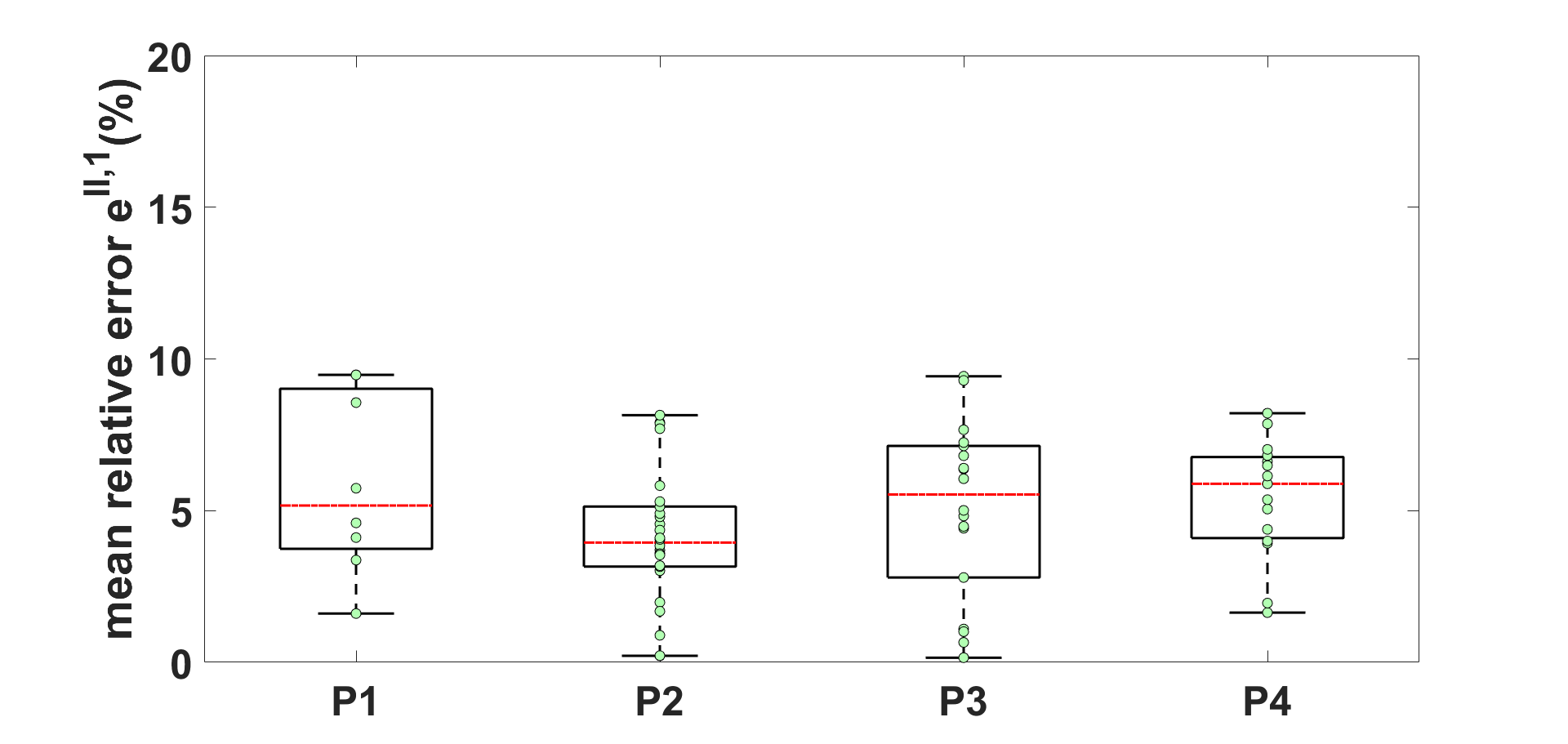
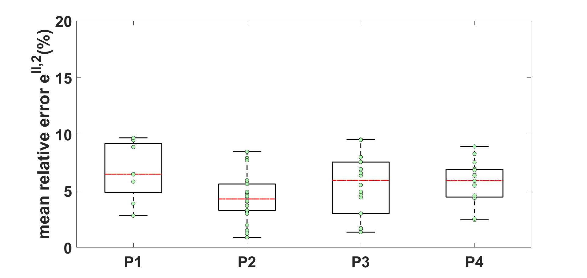
From these results, we observe an excellent quantitative agreement between epicardial vein measurements not used in the parameter estimation (group II) and our computed results. The mean error was in any case below ( if is considered) and the standard deviation confirmed a low error variability. Moreover, from the statistical analysis reported in Figure 8, we can observe that the errors are quite well confined in a small region, the maximum relative error being in any case less than 10%.
To complete the analysis, in Figure 9 we report the correlation plots between activation times obtained by numerical simulations and measurements. The corresponding slope of the regression fitting straight line and the coefficient of determination are shown in Table 5. We remember that provides a measure of how well observed outcomes are replicated by the model [63]. is generally considered strong effect size, whereas is generally considered a moderate effect size [23]. From our results, we observe a slope close to for all the patients and a coefficient of determination which features a strong effect size in 3 of the 4 patients, and a moderate effect size (very close to ) in 1 case.


3.2 Sensitivity of optimization with respect to some parameters
In order to highlight the sensitivity of our optimization procedure with respect to the choice of some parameters, we performed some further numerical experiments obtained by considering different scenarios. In particular:
- -
Test B: Absence of cardiac fibers and different fibers boundary angles;
- -
Test C: Different registration between electrical and geometric data;
- -
Test D: Different number of points in group I;
In order to highlight the importance of including the fibers orientations in the search of optimal conductivities, we solved the minimization problem (10) for a case without fibers, where we have only one value of the conductivity. In Table 6 we report the values of the optimal conductivity and the corresponding relative error with respect to group II for P3. From these results we observe the importance of including a suitable orientation of cardiac fibers to obtain accurate estimation of the conductivities
| [] | [] | ||||
|---|---|---|---|---|---|
| 1.23 | 0.25 | 0.07 | 1.13 | 5.05 | 7.93 |
In order to go deeper in the analysis of the influence of cardiac fibers orientation on the results of the minimization problem, we solved problem (10) for other two boundary values for the fibers in the Laplace-Dirichlet rule-based algorithm, that is and , the values of the sheets angles being the same of above. In Table 7 we reported the optimized conductivities and mean relative error for P3. From these results we observe that the value produces the smallest errors among the three choices.
| Fibers angle | [] | |||
|---|---|---|---|---|
| 1.12 | 0.22 | 0.07 | 7.67 | |
| 1.23 | 0.25 | 0.07 | 5.05 | |
| 1.36 | 0.27 | 0.07 | 7.55 |
As observed in Sect. 2.2.2, the merging of electrical and geometric data was based on the a priori selection of some reference points. This choice was guided by the anatomy of the patient (coronary sinus and septum) but it could be affected at a certain extent by an arbitrariness having an impact on the results. To investigate this point, we considered for P3 another configuration (perturbed scenario), where the reference points were located as much as possible far from the original ones, although satisfying anatomical requirements, see Figure 10, left.

As observed by the activation maps reported in Figure 10, right, there is a good agreement between measured and computed data also in the perturbed scenario. In fact, the different location of the septal reference points induces a rigid translation of all the other measures, so that it is not surprising that the qualitative propagation map is still well fitting the data. This is confirmed by the errors for data groups I and II reported in Table 8, which show almost identical values, suggesting the robustness of our analysis with respect to the arbitrariness of the data merging procedure.
| Scenario | [] | [] |
|---|---|---|
| standard | 6.90 | 5.05 |
| geometric perturbed | 6.84 | 5.10 |
| 6.59 | 5.11 | |
| 6.32 | 5.15 |
We want now to assess the importance of the number of points of group I used to calibrate the conduction velocities on the accuracy of the optimization procedure. To this aim, we considered for P3 2 further scenarios obtained by using 15 and 12 points (19 were used in the standard scenario). In Table 8 we reported the corresponding errors, obtained after the same optimization procedure that led to the same values of conductivities of the standard scenario. These errors highlight the robustness of the method with respect to the number of mapped points.
4 Discussion
4.1 General discussion of the results
In this paper we have performed an important step towards the validation of the monodomain model in the context of a normal ventricular sinus rhythm (i.e. without chaotic patterns) by using in-vivo data of activation times acquired in four patients. At the best of authors knowledge, this is the first validation attempt of the monodomain model where measured ventricular activation maps in humans are used to estimate conduction parameters and assess the errors in a cross-validation test.
Specifically, for each of the four cases considered, we have used patient-specific electrical data acquired at the septum to provide an input which is suitable for LBBB patients. We used a set of measures at the epicardial veins to calibrate the three conductivities and another one at the same location to quantify the error of the numerical results. The mean error found in this cross-validation test was in any case less than 6.2%, see also Figures 7, 8 and Table 5, and was comparable with that obtained for group I (see Table 4).This proves the robustness of the minimization problem for the data we had at disposal. From Table 2 we also notice that for P2 and, especially, for P3 and P4 our accurate results were found by using few input data (septal measurements). This means that it is enough to have at disposal very few measurements of activation times where the signal starts in order to well predict the activation in the epicardial veins.
The validation against epicardial measures is particularly significant. Indeed, the front propagating from the endocardium activates all the myocardium before reaching the epicardium, thus assessing the accuracy of the results at the epicardium means accounting for the reliability of the propagation in all the myocardium. Among the studies which incorporates epicardial measures in computational models, only [8], together with the present study, considered measures at the epicardial veins. Some differences of the present work with respect to [8] are the use of monodomain model instead of the reaction-Eikonal one, the simulation of a sinus rhythm instead of a stimulated scenario (at the right ventricle apex), the use of patient specific input data at the septum, and the calibration against epicardial activation times instead of ECG measures.
Our modeling choice was oriented towards the monodomain model, at the expense of an increased computational time with respect, e.g., to the Eikonal models. This was motivated by the fact that the monodomain model should be more accurate. Indeed, although the Eikonal equation was seen to be accurate in predicting the activation time, it is a reduced model of the monodomain one [53] and thus introduces an error in the computation of the activation times with respect to monodomain. For example, in [46], such discrepancy has been quantified to be about 10%. Moreover, the monodomain model allowed us to compute also the transmembrane potential and thus to provide supplementary clinical information. Additionally, the monodomain model will be fundamental for electro-mechanical simulations to effectively assess the functioning of CRT. An alternative choice could be provided by the reaction-Eikonal model [3, 8], which at some extent merges Eikonal and monodomain models. This method has a good accuracy (discrepancies with respect to the bidomain model in any case less than 20%, with about 33% of the points affected by an error smaller than 2.5%) and very good computational times, which are intermediate between Eikonal and monodomain. Moreover, unlike Eikonal this model is able to provide the transmembrane potential. It will however be interesting for further studies to assess if any differences between reaction-Eikonal and monodomain model would be significantly out-weighted by other errors in the simulation pipeline (registration errors, inaccurate representation of fibre architecture, for example).
Results in Table 6 and 7 showed the importance of including a suitable cardiac fibers orientation when looking for optimal values of the conductivities to accurately match the clinical measurements. In particular, although and are acceptable boundary values for fibers angle falling in the physiological range [28], the value produced the smallest errors, confirming the validity of this choice as proven by the hystological studies in [48]. Moreover, the absence of any fibers, due to the simplified model (only one parameter instead of three to estimate) led to error about 60% greater than in the case with a suitable cardiac fibers field.
Some of the results presented are, at the best of authors knowledge, completely new in the field of computational electro-physiology. First, we highlight that this is the first cross-validation analysis against clinical measures of ventricular activation times. Second, for the first time we used measures at the epicardial veins to validate the monodomain equation. This is particularly relevant since the signal usually originates at the endocardial level. Finally, we included some results about the sensitivity of the solution of the minimization problem with respect to the cardiac fibers orientation.
4.2 Possible clinical implications
The previous findings could be of some interest for clinical applications. For example, in view of CRT cardiologists often use the point with the latest activation time (LAT) at the epicardial veins to locate the left electrode [26, 71]. Then, thanks to our accurate numerical method, this information can be in principle provided without a complete mapping of the epicardial veins, shortening the invasive procedure based on the insertion of catheters (up to a couple of hours) and reduce the exposition of the patient to radiation. For example, only the mapping of the coronary sinus could be in principle provided to obtain the data needed for the calibration. This mapping is in general quite ”simple” to perform since the coronary sinus is easily detectable and in the most proximal region.
As observed, the choice of using the earliest (proximal) and latest (distal) activated points for the calibration and validation groups, respectively, allowed us to avoid overlaps and obtain more significant results. Moreover, this could be of particular clinical interest, since one could acquire only the earliest (most accessible) activated points, e.g. those in the coronary sinus, and computationally estimate (without the need of mapping) the deepest ones, where LAT occurs. In this way there is no need to push the catheter deeper in the veins, where the activation times could be completely predicted by our computational method, yielding a potential benefit for the patient. This has been emphasized from the analysis of Test C (see Table 8) where we stressed the need of few points (for example the more proximal ones on the coronary sinus) to be acquired by the mapping procedure in order to have an accurate calibration. Moreover, all the epicardial surface could be virtually mapped. This would allow to find the global LAT (i.e. the latest among all the epicardial points, not only those in the veins) which could be useful for surgical implantation of the left electrode [34, 43].
The effective applications of the monodomain model for such purposes is however nowadays a little bit problematic since the implantation of CRT and the mapping procedure happen during the same day and computational costs of monodomain are still of several hours, thus requiring high performance computing resources. However, this strategy could be effective in few years owing to the development of more performing computing resources, new preconditioners, and implementation of faster optimization strategy.
Another important possible clinical implication made possible by the use of a validated monodomain model is the electrical-mechanical (EM) virtual study of CRT where the left electrode is placed on the computed LAT. Nowadays, this application would be limited to case studies due to the high computational time of EM simulations. However, this could provide useful information about the effective validity of LAT as stimulation point able to provide a restored heart function.
4.3 Limitations
Some limitations affected the present study.
The first one consisted, as observed, in the absence of any model for the Purkinje system, both in terms of reconstruction of a suitable network and by surrogating its effect increasing the LV subendocardium conduction [41], as done first in [38] and then also, e.g., in [8].
Another limitation of the current work consists in the comparison of numerical results only against sparse activation points. A more complete validation could in future be obtained by using full endocardial or epicardial maps. This however will require specific acquisition protocols since full maps are usually outside the standard clinical practice. Also, when available, the comparison with repolarization maps and not only with activation times will be mandatory to complete the validation of monodomain model.
We also mention that here we focused only on data of sinus rhythm, thus we did not validate restitution properties of the model and pathological scenarios. Cross-validations against measures obtained under suitable stimulus protocols and for arrhythmic cases are mandatory to complete our work.
Another limitation is the use of the left ventricle solely, instead of a biventricular model as done in [8]. The inclusion of the right ventricle will be mandatory in electro-mechanical studies for CRT applications. We notice however that, since we are interested here in predicting the results in the left ventricle epicardium, the absence of the right ventricle geometry should not affect the results. This was motivated by the fact that we used patient-specific electrical data at the septum as input for the left ventricle activation.
We finally mention the fact that we did not address the issue of quantifying the geometric projection error obtained when merging the electrical data from Ensite Precision system with the epicardial surface of the ventricle, see Figure 3. Currently, we are investigating how much this error can affect our error analysis.
Acknowledgements
This project has received funding from the European Research Council (ERC) under the European Union’s Horizon 2020 research and innovation programme (grant agreement No 740132, iHEART - An Integrated Heart Model for the simulation of the cardiac function, P.I. Prof. A. Quarteroni). CV has been partially supported also by the H2020-MSCA-ITN-2017, EU project 765374 "ROMSOC - Reduced Order Modelling, Simulation and Optimization of Coupled systems". AQ and CV have been partially supported also by the Italian research project MIUR PRIN17 2017AXL54F "Modeling the heart across the scales: from cardiac cells to the whole organ".
References
- [1] Barone A., Gizzi A., Fenton F., Filippi S., and Veneziani A. Experimental validation of a variational data assimilation procedure for estimating space-dependent cardiac conductivities. Computer Methods in Applied Mechanics and Engineering, 358:112615, 2020.
- [2] Bueno-Orovio A., Cherry E.M., and Fenton F.H. Minimal model for human ventricular action potentials in tissue. Journal of Theoretical Biology, 253(3):544–560, 2008.
- [3] Neic A., Campos F.O., Prassl A.J., Niederer S.A., Bishop M.J., Vigmond E.J., and Plank G. Efficient computation of electrograms and ECGs in human whole heart simulations using a reaction-eikonal model. Journal of Computational Physics, 346:191–211, 2017.
- [4] Quarteroni A., Dede’ L., Manzoni A., and Vergara C. Mathematical Modelling of the Human Cardiovascular System-Data, Numerical Approximation, Clinical Applications. Cambridge University Press, 2019.
- [5] Hodgkin A.L. and Huxley A.F. A quantitative description of membrane current and its application to conduction and excitation in nerve. The Journal of Physiology, 117(4):500–544, 1952.
- [6] Muzikant A.L., Hsu E.W., Wolf P.D., and Henriquez C.S. Region specific modeling of cardiac muscle: Comparison of simulated and experimental potentials. Annals of Biomedical Engineering, 30(7):867–883, 2002.
- [7] Pop M .and Sermesant M., Flor R., Pierre C., Mansi T., Oduneye S., Barry J., Coudiere Y., Crystal E., Ayache N., and Wright G.A. In vivo contact EP data and ex vivo MR-based computer models: Registration and model-dependent errors. In Statistical Atlases and Computational Models of the Heart. Imaging and Modelling Challenges, pages 364–374. Springer Berlin Heidelberg, 2013.
- [8] Lee A.W.C., Nguyen U.C., Razeghi O., Gould J., Sidhu B.S., Sieniewicz B., Behar J., Mafi-Rad M., Plank G., Prinzen F.W., Rinaldi C.A., Vernooy K., and Niederer S. A rule-based method for predicting the electrical activation of the heart with cardiac resynchronization therapy from non-invasive clinical data. Medical Image Analysis, 57:197–213, 2019.
- [9] Corrado C., Gerbeau J.F., and Moireau P. Identification of weakly coupled multiphysics problems. application to the inverse problem of electrocardiography. J. Comput. Phys., 283:271–298, 2015.
- [10] Corrado C., Williams S., Karim R., Plank G., O’Neill M., and Niederer S. A work flow to build and validate patient specific left atrium electrophysiology models from catheter measurements. Medical Image Analysis, 47:153–163, 2018.
- [11] Costa C., Hoetzl E., Rocha B.M., Prassl A.J., and Plank G. Automatic parameterization strategy for cardiac electrophysiology simulations. Computing in Cardiology, 40:373–376, 2013.
- [12] Eitel C., Hindricks G., Dagres N., Sommer P., and Piorkowski C. EnSite velocity™ cardiac mapping system: a new platform for 3d mapping of cardiac arrhythmias. Expert Review of Medical Devices, 7(2):185–192, 2010.
- [13] Sánchez C., D’Ambrosio G., Maffessanti F., Caiani E.G., F. W. Prinzen F.W., Krause R., Auricchio A., and Potse M. Sensitivity analysis of ventricular activation and electrocardiogram in tailored models of heart-failure patients. Medical & Biological Engineering & Computing, 56(3):491–504, 2017.
- [14] Vergara C., Lange M., Palamara S., Lassila T., Frangi A.F., and Quarteroni A. A coupled 3D-1D numerical monodomain solver for cardiac electrical activation in the myocardium with detailed Purkinje network. J. Comput. Phys, 308:218–238, 2016.
- [15] Vergara C., Palamara S., Catanzariti D., Nobile F., Faggiano E., C. Pangrazzi, Centonze M., Maines M., Quarteroni A., and Vergara G. Patient-specific generation of the Purkinje network driven by clinical measurements of a normal propagation. Med. Biol. Eng. Comput., 52(10):813–826, 2014.
- [16] Augustin C.M., Crozier A., Neic A., Prassl A.J., Karabelas E., Ferreira da Silva T., Fernandes J.F., Campos F., Kuehne T., and Plank G. Patient-specific modeling of left ventricular electromechanics as a driver for haemodynamic analysis. EP Europace, 18(suppl_4):iv121–iv129, 2016.
- [17] Augustin C.M., Neic A., Liebmann M., Prassl A.J., Niederer S.A., Haase G., and Plank G. Anatomically accurate high resolution modeling of human whole heart electromechanics: A strongly scalable algebraic multigrid solver method for nonlinear deformation. Journal of Computational Physics, 305:622–646, 2016.
- [18] Arndt D., Bangerth W., Clevenger T.C., Davydov D., Fehling M., Garcia-Sanchez D., Harper G., Heister T., Heltai L., Kronbichler M., Kynch R.M., Maier M., Pelteret J.-P., Turcksin B., and Wells D. The deal.II library, version 9.1. Journal of Numerical Mathematics, 2019. accepted.
- [19] Deng D., Arevalo H., Pashakhanloo F., Prakosa A., Ashikaga H., McVeigh E., Halperin H., and Trayanova N. Accuracy of prediction of infarct-related arrhythmic circuits from image-based models reconstructed from low and high resolution MRI. Frontiers in Physiology, 6, 2015.
- [20] Hurtado D.E. and Rojas G. Non-conforming finite-element formulation for cardiac electrophysiology: an effective approach to reduce the computation time of heart simulations without compromising accuracy. Computational Mechanics, 61(4):485–497, 2017.
- [21] Roberts D.E. and Scher A.M. Effect of tissue anisotropy on extracellular potential fields in canine myocardium in situ. Circulation Research, 50(3):342–351, 1982.
- [22] Roberts D.E., Hersh L.T., and Scher A.M. Influence of cardiac fiber orientation on wavefront voltage, conduction velocity, and tissue resistivity in the dog. Circulation Research, 44(5):701–712, 1979.
- [23] Moore D.S., Notz W.I, and Flinger M.A. The basic practice of statistics (6th ed.). W. H. Freeman and Company, New York, 2013.
- [24] Konukoglu E., Relan J., Cilingir U., Menze B.H., Chinchapatnam P., Jadidi A., Cochet H., Hocini M., Delingette H., Jaïs P., Haïssaguerre M., Ayache N., and Sermesant M. Efficient probabilistic model personalization integrating uncertainty on data and parameters: Application to eikonal-diffusion models in cardiac electrophysiology. Progress in Biophysics and Molecular Biology, 107(1):134–146, 2011.
- [25] Vigmond E.J. and Clements C. Construction of a computer model to investigate sawtooth effects in the Purkinje system. IEEE Trans Biomed Eng, 54(3):389–399, 2007.
- [26] Zanon F., Baracca E., Pastore G., Fraccaro C., Roncon L., Aggio S., Noventa F., Mazza A., and Prinzen F. Determination of the longest intrapatient left ventricular electrical delay may predict acute hemodynamic improvement in patients after cardiac resynchronization therapy. Circulation: Arrhythmia and Electrophysiology, 7(3):377–383, 2014.
- [27] Lines G.T., MacLachlan M.C., Linge S., and Tveito A. Synchronizing computer simulations with measurement data for a case of atrial flutter. Ann Biomed Eng, 37:1287–1293, 2009.
- [28] Lombaert H., Peyrat J., Croisille P., Rapacchi S., Fanton L., Cheriet F., Clarysse P., Magnin I., Delingette H., and Ayache N. Human atlas of the cardiac fiber architecture: Study on a healthy population. IEEE Transactions on Medical Imaging, 31(7):1436–1447, 2012.
- [29] Yang H. and Veneziani A. Efficient estimation of cardiac conductivities via POD-DEIM model order reduction. Applied Numerical Mathematics, 115:180–199, 2017.
- [30] Arevalo H.J., Vadakkumpadan F., Guallar E., Jebb A., Malamas P., Wu K.C., and Trayanova N.A. Arrhythmia risk stratification of patients after myocardial infarction using personalized heart models. Nature Communications, 7(1), 2016.
- [31] Relan J., Pop M., Delingette H., Wright G.A., Ayache N., and Sermesant M. Personalization of a cardiac electrophysiology model using optical mapping and MRI for prediction of changes with pacing. IEEE Transactions on Biomedical Engineering, 58(12):3339–3349, 2011.
- [32] Bayer J.D., Blake R.C., Plank G., and Trayanova N.A. A novel rule-based algorithm for assigning myocardial fiber orientation to computational heart models. Annals of Biomedical Engineering, 40(10):2243–2254, 2012.
- [33] Stinstra J.G., Hopenfeld B., and MacLeod R.S. On the passive cardiac conductivity. Annals of Biomedical Engineering, 33(12):1743–1751, 2005.
- [34] Navia J.L., Atik F.A., Grimm R.A., Garcia M., Vega P.R., Myhre U., Starling R.C., Wilkoff B.L., Martin D., Houghtaling P.L., Blackstone E.H., and Cosgrove D.M. Minimally invasive left ventricular epicardial lead placement: Surgical techniques for heart failure resynchronization therapy. The Annals of Thoracic Surgery, 79(5):1536–1544, 2005.
- [35] Ten Tusscher K.H.W.J., Mourad A., Nash M.P., Clayton R.H., Bradley C.P., Paterson D.J., Hren R., Hayward M., Panfilov A.V., and Taggart P. Organization of ventricular fibrillation in the human heart: experiments and models. Experimental Physiology, 94(5):553–562, 2009.
- [36] Andrews L. A template for the nearest neighbor problem. C/C++ Users Journal, 19(11):40–49, 2008.
- [37] Antiga L., Piccinelli M., Botti L., Ene-Iordache B., Remuzzi A., and Steinman D.A. An image-based modeling framework for patient-specific computational hemodynamics. Medical & Biological Engineering & Computing, 46(11):1097–1112, 2008.
- [38] Cardone-Noott L., Bueno-Orovio A., Mincholé A., Zemzemi N., and Rodriguez B. Human ventricular activation sequence and the simulation of the electrocardiographic QRS complex and its variability in healthy and intraventricular block conditions. EP Europace, 18(suppl_4):iv4–iv15, 2016.
- [39] Clerc L. Directional differences of impulse spread in trabecular muscle from mammalian heart. The Journal of Physiology, 255(2):335–346, 1976.
- [40] Wang L., Dawoud F., Yeung S., Shi P., Wong K.C.L., Liu H., and Lardo A.C. Transmural imaging of ventricular action potentials and post-infarction scars in swine hearts. IEEE Transactions on Medical Imaging, 32(4):731–747, 2013.
- [41] Draper M. and Mya-Tu M. A comparison of the conduction velocity in cardiac tissues of various mammals. Exp Physiol, 44:91–109, 1959.
- [42] Fedele M. Polygonal surface processing and mesh generation tools for numerical simulations of the complete cardiac function. MOX Report 32, Politecnico di Milano, 2019.
- [43] Marini M., Branzoli S., Moggio P., Martin M., Belotti G., Molon G., Guarracini F., Coser A., Quintarelli S., Pederzolli C., Graffigna A., Penzo D., Valsecchi S., Bottoli M.C., Pepi P., Bonmassari R., and Droghetti A. Epicardial left ventricular lead implantation in cardiac resynchronization therapy patients via a video-assisted thoracoscopic technique: Long-term outcome. Clinical Cardiology, 43(3):284–290, 2019.
- [44] Potse M., Dube B., Richer J., Vinet A., and Gulrajani R.M. A comparison of monodomain and bidomain reaction-diffusion models for action potential propagation in the human heart. IEEE Transactions on Biomedical Engineering, 53(12):2425–2435, 2006.
- [45] Sermesant M., Chabiniok R., Chinchapatnam P., Mansi T., Billet F., Moireau P., Peyrat J.M., Wong K., Relan J., Rhode K., Ginks M., Lambiase P., Delingette H., Sorine M., Rinaldi C.A., Chapelle D., Razavi R., and Ayache N. Patient-specific electromechanical models of the heart for the prediction of pacing acute effects in CRT: A preliminary clinical validation. Medical Image Analysis, 16(1):201–215, 2012.
- [46] Wallman M., Smith N.P, and Rodriguez B. A comparative study of graph-based, eikonal, and monodomain simulations for the estimation of cardiac activation times. IEEE Transactions on Biomedical Engineering, 59(6):1739–1748, 2012.
- [47] Fernández M.A. and Zemzemi N. Decoupled time-marching schemes in computational cardiac electrophysiology and ECG numerical simulation. Mathematical Biosciences, 226(1):58–75, 2010.
- [48] Toussaint N., Stoeck C.T., Schaeffter T., Kozerke S., Sermesant M., and Batchelor P.G. In vivo human cardiac fibre architecture estimation using shape-based diffusion tensor processing. Medical Image Analysis, 17(8):1243–1255, 2013.
- [49] Camara O., Sermesant M., Lamata P., Wang L., Pop M., Relan J., De Craene M., Delingette H., Liu H., Niederer S., Pashaei A., Plank G., Romero D., Sebastian R., Wong K.C.L., Zhang H., Ayache N., Frangi A.F., Shi P., Smith N.P., and Wright G.A. Inter-model consistency and complementarity: Learning from ex-vivo imaging and electrophysiological data towards an integrated understanding of cardiac physiology. Progress in Biophysics and Molecular Biology, 107(1):122–133, 2011.
- [50] Dössel O., Krueger M.W., Weber F.M., Wilhelms M., and Seemann G. Computational modeling of the human atrial anatomy and electrophysiology. Med. Biol. Eng. Comput, 50:773–799, 2008.
- [51] German Cancer Research Center Division of Medical Image Computing. Medical imaging interaction toolkit. http://www.mitk.org/wiki/MITK, 2015.
- [52] Chinchapatnam P., Rhode K.S., Ginks M., Rinaldi C.A., Lambiase P .and Razavi R., Arridge S., and Sermesant M. Model-based imaging of cardiac apparent conductivity and local conduction velocity for diagnosis and planning of therapy. IEEE Trans. Med. Imaging, 27:1631–1642, 2008.
- [53] Colli Franzone P., Guerri L., and Rovida S. Wavefront propagation in an activation model of the anisotropic cardiac tissue: asymptotic analysis and numerical simulations. Journal of Mathematical Biology, 28:121–176, 1990.
- [54] Colli Franzone P., Pavarino L.F., and Taccardi B. Simulating patterns of excitation, repolarization and action potential duration with cardiac bidomain and monodomain models. Mathematical Biosciences, 197(1):35–66, 2005.
- [55] Colli Franzone P., Pavarino L.F., and Savaré G. Computational electrocardiology: mathematical and numerical modeling. In Complex Systems in Biomedicine, pages 187–241. Springer Milan, 2006.
- [56] Colli Franzone P., Pavarino L.F., and Scacchi S. Mathematical Cardiac Electrophysiology. Springer International Publishing, 2014.
- [57] Le Guyader P., Trelles F., and Savard P. Extracellular measurement of anisotropic bidomain myocardial conductivities. i. theoretical analysis. Annals of Biomedical Engineering, 29(10):862–877, 2001.
- [58] Pathmanathan P., Bernabeu M.O., Niederer S., Gavaghan D.J., and Kay D. Computational modelling of cardiac electrophysiology: explanation of the variability of results from different numerical solvers. International journal for numerical methods in biomedical engineering, 28(8):890–903, 2012.
- [59] Bordas R., Gillow K., Lou Q., Efimov I.R., Gavaghan D., Kohl P., Grau V., and Rodriguez B. Rabbit-specific ventricular model of cardiac electrophysiological function including specialized conduction system. Progress in Biophysics and Molecular Biology, 107(1):90–100, 2011.
- [60] Doste R., Soto-Iglesias D., Bernardino G., Alcaine A., Sebastian R., Giffard-Roisin S., Sermesant M., Berruezo A., Sanchez-Quintana D., and Camara O. A rule-based method to model myocardial fiber orientation in cardiac biventricular geometries with outflow tracts. International Journal for Numerical Methods in Biomedical Engineering, 35(4):e3185, 2019.
- [61] Piersanti R., Africa P.C., Fedele M., Vergara C., Dede’ L., Corno A.F., and Quarteroni A. Numerical methods for generating cardiac muscle fibersin ventricular and atrial electrophysiology simulation. MOX Report 29, Politecnico di Milano, 2020.
- [62] Sebastian R., Ordas S., Plank G., Rodriguez B., Vigmond E.J., and Frangi A.F. Assessing influence of conductivity in heart modelling with the aim of studying cardiovascular diseases. In Xiaoping P. Hu and Anne V. Clough, editors, Medical Imaging 2008: Physiology, Function, and Structure from Medical Images. SPIE, 2008.
- [63] Steel R.G.D. and Torrie J.H. Principles and Procedures of Statistics with Special Reference to the Biological Sciences. McGraw Hill, New York, 1960.
- [64] Bordas R.M., Gillow K., Gavaghan D., Rodríguez B., and Kay D. A Bidomain model of the ventricular specialized conduction system of the heart. SIAM J. Appl. Math., 72(5):1618–1643, 2012.
- [65] Krishnamoorthi S., Perotti L.E., Borgstrom N.P., Ajijola O.A., Frid A., Ponnaluri A.V., Weiss J.N., Qu Z., Klug W.S., Ennis D.B., and Garfinkel A. Simulation methods and validation criteria for modeling cardiac ventricular electrophysiology. PLoS ONE, 9(12):e114494, 2014.
- [66] Krishnamoorthi S., Sarkar M., and Klug W.S. Numerical quadrature and operator splitting in finite element methods for cardiac electrophysiology. International journal for numerical methods in biomedical engineering, 29(11):1243–1266, 2013.
- [67] Niederer S., Kerfoot E., Benson A.P., Bernabeu M.O., Bernus O., Bradley C., Cherry E.M., Clayton R., Fenton F., Garny A., Heidenreich E., Land S., Maleckar M., Pathmanathan P., Plank G., Rodrìguez J.F., Roy I., Sachse F.B., Seemann G., Skavhaug O., and Smith N.P. Verification of cardiac tissue electrophysiology simulators using an n -version benchmark. Philosophical Transactions of the Royal Society A: Mathematical, Physical and Engineering Sciences, 369(1954):4331–4351, 2011.
- [68] Niederer S., Plank G., Chinchapatnam P., Ginks M., Lamata P., Rhode K.S., Rinaldi C.A., Razavi R., and Smith N.P. Length-dependent tension in the failing heart and the efficacy of cardiac resynchronization therapy. Cardiovascular Research, 89(2):336–343, 2010.
- [69] Palamara S., Vergara C., Catanzariti D., Faggiano E., Pangrazzi C., Centonze M., Nobile F., Maines M., and Quarteroni A. Computational generation of the Purkinje network driven by clinical measurements: the case of pathological propagations. Int. J. Numer. Meth. Biomed. Engng., 30(12):1558–1577, 2014.
- [70] Gurev V., Lee T., Constantino J., Arevalo H., and Trayanova N.A. Models of cardiac electromechanics based on individual hearts imaging data. Biomechanics and Modeling in Mechanobiology, 10(3):295–306, 2010.
- [71] Liang Y., Yu H., Zhou W., Xu G., Sun Y., Liu R., Wang Z., and Han Y. Left ventricular lead placement targeted at the latest activated site guided by electrophysiological mapping in coronary sinus branches improves response to cardiac resynchronization therapy. Journal of Cardiovascular Electrophysiology, 26(12):1333–1339, 2015.
- [72] Saad Y. and Schultz M.H. Gmres: A generalized minimal residual algorithm for solving nonsymmetric linear systems. SIAM Journal on scientific and statistical computing, 7(3):856–869, 1986.