A greedy chip-firing game
Abstract.
We introduce a deterministic analogue of Markov chains that we call the hunger game. Like rotor-routing, the hunger game deterministically mimics the behavior of both recurrent Markov chains and absorbing Markov chains. In the case of recurrent Markov chains with finitely many states, hunger game simulation concentrates around the stationary distribution with discrepancy falling off like , where is the number of simulation steps; in the case of absorbing Markov chains with finitely many states, hunger game simulation also exhibits concentration for hitting measures and expected hitting times with discrepancy falling off like rather than . When transition probabilities in a finite Markov chain are rational, the game is eventually periodic; the period seems to be the same for all initial configurations and the basin of attraction appears to tile the configuration space (the set of hunger vectors) by translation, but we have not proved this.
Key words and phrases:
chip-firing, recurrence, stationary distribution1. Introduction
In the 1970s, Arthur Engel [5, 6] introduced a “stochastic abacus” that deterministically mimics many aspects of the behavior of finite-state Markov chains with rational probabilities. Unaware of Engel’s work, various mathematicians and physicists invented and studied the abelian sandpile model [4] and the chip-firing game [1] which in many respects embody the same core idea as Engel’s abacus but with different motivations. For books surveying chip-firing we refer readers to [11, 2].
In the 2010s, inspired by Engel’s work, the second author of this paper in collaboration with Ander Holroyd [8] introduced a different way to deterministically mimic Markov chains via “rotor-routing” (unaware that physicists were already studying the process under the name “the Eulerian walkers model” [13]). The emphasis of much of this work on the rotor-router model, inspired by discrepancy theory and quasi-Monte Carlo methods, was on the fidelity of the deterministic process to the associated Markov chain. Specifically, it was shown that for certain asymptotically-defined quantities associated with Markov chains (e.g., the proportion of the time that the chain spends in a specific state), rotor-router simulation has the same limiting behavior as the Markov chain, typically with faster convergence than the Markov chain itself would typically exhibit. For a comprehensive background on chip-firing and rotor-routing and the relationship between them, we refer readers to [7].
Here we discuss another way to derandomize Markov chains which we call the hunger game. It can be applied to any discrete-state discrete-time Markov chain, whether or not the transition probabilities are rational. (Rotor-routing can be extended to this regime — see the discussion of stack walks in [8] — though we know of no way to extend chip-firing in this direction.) A key difference between rotor-routing and the hunger game is that the frequency with which state is followed by in rotor-router simulation converges to the transition probability ; this is not the case for the hunger game. That is, the hunger game does not exhibit fidelity with regard to transition-frequencies. However, we believe this may be a virtue rather than a vice, as we will explain in the concluding section.
In Section 2 we define the hunger game and the chip addition operators associated with it. In Section 3 we prove fundamental results on the boundedness of hunger, and in Section 4 we prove basic results on the behavior of chip addition operators. In Section 5 we prove the main result of this paper, demonstrating that the normalized firing vector of a hunger game process converges to the unique stationary distribution of an irreducible Markov chain with a discrepancy bound inversely proportional to the number of time steps. We apply this result to show how the hunger game process can calculate hitting probability distributions, escape probabilities, expected absorption times, and expected return times in Section 6 . In Section 7 we focus on finite Markov chains with rational transition probabilities. We introduce the notion of a recurrent hunger vector (a vector that returns to itself under the hunger game) and study the properties of the basin of attraction (the set of recurrent vectors). In the case where all transition probabilities are rational, we prove the zero vector is always recurrent and determine its period, and conjecture that all the periods for a given Markov chain are the same. We conclude with Section 8 , comparing the discrepancies of the rotor-router model and the hunger game.
2. Preliminaries
See [9] or [12] for basic facts about Markov chains. Throughout this paper, except where otherwise noted, Markov chains are assumed to have a finite state space indexed by positive integers for some ; when we consider Markov chains with countably infinite state spaces, we will assume that for each state there are only finitely many states such that the transition probability from state to state is positive. We can represent a Markov chain by a weighted directed graph whose vertices are the allowed states and the weight of the directed edge is . For brevity, we will use the words state and vertex to refer to both the state in the Markov chain and the corresponding vertex in , passing back and forth between the abstract Markov chain and its concrete embodiment as a random walk on . We say that state is an absorbing state if (equivalently if has a loop at with weight 1). Notice that for every vertex , the sum of the weights of all edges is 1.
Let , where is the -by- identity matrix. Let , , and denote the th rows of the matrices , , and respectively. Observe that (the th unit vector) and that is the Laplacian of the graph. The Markov chain admits at least one stationary measure for which the vector satisfies (this follows from the assumption that the Markov chain is finite; see, e.g., [12]), so 1 is an eigenvalue of and 0 is an eigenvalue of . All eigenvalues of have magnitude at most 1. When the Markov chain is irreducible (that is, when every state can be reached from every other state in some finite number of steps), 1 is a simple eigenvalue of and 0 is a simple eigenvalue of , so that has rank , and the rows of , taken with integer coefficients, generate an -dimensional sublattice of the space of vectors with entries summing to zero; in this case, there is a unique stationary measure satisfying .
We now informally introduce the hunger game on the weighted directed graph by comparing it to the chip-firing model and the rotor-router model before offering a more technical definition.
The “goodness” of a deterministic analogue of a random process can be assessed by the notion of discrepancy. If some numerical characteristic of the deterministic process converges to a corresponding numerical characteristic of the random process as simulation time goes to infinity, one can try to determine the rate of convergence.
The simplest deterministic analogues of Markov chains were invented by Engel [5, 6], under the name the stochastic abacus (though the term chip-firing is more common nowadays). Suppose that all the transition probabilities are rational, and that we have positive integers such that is an integer for all . Assume that the Markov chain is irreducible. Define a chip-configuration as an -tuple ; say that a chip-configuration is stable if whenever is a non-absorbing state. If , then we obtain another chip-configuration by firing at , replacing by ; if we represent the Markov chain by drawing a graph with vertices and we represent the chip-configuration by putting chips at for all , then firing means sending chips from to for each . Chip-firing can be used to find the stationary probability measure of an irreducible Markov chain as follows. Put sufficiently many chips on the state-graph so that stabilization is impossible no matter how many firings are performed, and start performing firings however one wishes; when we encounter a chip-configuration we have seen before (as must happen eventually), the vector that records the number of times each state has fired will be a stationary vector.
Example 2.1.
Suppose we have the Markov chain given by the Markov matrix
representing a doubly-reflecting random walk. Its corresponding graph is shown in Fig. 1 .
If we place 1 chip at state 1, 2 chips at state 2, and 1 chip at state 3, then state 2 is unstable, so we may fire at 2, turning the chip-configuration (1,2,1) into the chip-configuration (2,0,2). Then firing at 1 and at 3 brings us back to (1,2,1). The vector that records the number of times each state fired is (1,1,1), which is indeed a stationary vector for this Markov chain.
The rotor-router model [8] is a different scheme for imitating Markov chains deterministically. Assume as above that the Markov chain has rational transition probabilities, with as above. Represent the Markov chain using a directed graph with parallel edges from to , so that has outdegree . Each vertex distributes arriving chips along its outgoing edges in a cyclic manner, not sending a chip along any edge for a second time until it has sent a chip along every edge at least once, and thereafter always sending the next chip along the edge along which it has sent a chip least recently. Inasmuch as the vertex with the chip gets to decide where the chip goes next, we call this “supply-side” management of the chip’s movement. Assume that the Markov chain is irreducible. It can be shown that once the chip enters an infinite loop (as must happen eventually), the fraction of the time that the chip spends at vertex is proportional to the steady-state .
Example 2.2.
We use the same Markov chain as Example 2.1. Suppose we start with the chip at and begin the game by sending the chip to , then , then again. Since at this point the chip has already traveled along the edge sending to , it now travels along the edge from to . As the chip has already gone from to , the rotor-router protocol dictates that it must now travel along the other edge from and go to . Similarly, as it has already gone from to , now it must travel from to . Thereafter the process cycles forever. Since within each cycle the chip spends 2 steps at each vertex, (2,2,2) is a stationary vector.
The hunger game introduced in this article can be seen as a “demand-side” management system: each vertex has a “hunger” for chips, determined by its expectation of receiving chips from neighboring vertices that have been previously visited. When a vertex receives a chip, the neighboring vertices’ hunger increases in accordance to the transition probabilities from to those vertices, and sends its chip to the vertex with highest hunger (regardless of whether that chip is a neighbor of ).
Now we give a more formal definition of the hunger game. It is simplest to start with the situation in which the chain runs forever without restarts (in contrast to chains that will be restarted when they enter an absorbing state). We also start with the case in which the state space is finite, with , deferring discussion of infinite-state spaces until later. The hunger vector represents the hunger at each vertex in ; we will sometimes call it the hunger state to emphasize its interpretation as a state of the hunger game system. At each step, whichever vertex has the highest hunger receives the chip; if vertex receives the chip, then the hunger vector is updated by adding to it, corresponding to the increase in vertices’ hunger from the presence of this chip at but also the satiation of after receiving a chip. If multiple states are tied for the highest hunger, we break the tie by choosing the lowest-indexed such vertex. Since each row of has entries summing to 0, total hunger never changes.
Each relocation of the chip is referred to as firing the chip; specifically, when the chip is relocated at , we say the chip fires to . Unlike rotor-router or chip-firing, under the hunger game rules a chip does not necessarily have to be fired to a vertex adjacent to its current location; see Example 2.3 . In fact, the determination of the chip’s next location depends only on the hunger state and not the current location of the chip. The step can be described purely in terms of the matrix and the vector without any reference to chips, via the rule “Replace by where maximizes , choosing the smallest such in the event of a tie.”
Example 2.3.
We use the same Markov chain as Example 2.1. Starting with , as shown in Fig. 2(a) , regardless of the initial location of the chip, we fire the chip to under the tie-breaking rule, yielding as shown in Fig. 2(b) . After this, we fire to , as shown in Fig. 2(c) , and then fire to , as shown in Fig. 2(d) . Notice that we have returned back to the initial hunger state , so this process repeats, visiting states 1, 2, 3, then back to 1, and so on. Notice that we fire the chip from 3 to 1 even though .
If one ignores the chip and focuses on the entries of the hunger vector, the hunger game can be viewed as a greedy variant of chip-firing. Specifically, if all entries of and are rational, we can without loss of generality assume they are all non-negative integers (since the firing rule is invariant under affine transformation of the hunger vector) and create a chip-configuration of the customary kind in which the number of chips at is . Then the firing rule, translated to the new context, tells us to fire the vertex that has the most chips, with ties resolved as before.
When the state space is (countably) infinite, our hunger vectors are infinite sequences. We restrict ourselves to sequences that are bounded and take on only finitely many distinct values; this ensures that there exists at least one for which equals , from which it follows that a smallest such exists. As each vertex has only finitely many outgoing edges, this assumption ensures that after any finite number of steps in the hunger game there are only finitely many distinct values of hunger, so a vertex of highest hunger can be found and the lowest-indexed one can be chosen, ad infinitum.
For Markov chains with absorbing states we vary the procedure slightly. We start with a graph devoid of chips, add a chip at an initial vertex, and then follow the rule for moving the chip described above, with the extra stipulation that when the chip reaches an absorbing vertex, it gets removed from the graph. In more detail, we define chip addition operators as follows: Given an initial hunger vector , we place a chip at (increasing the hunger of the neighbors of ) and add to , and we then repeatedly move the chip to the currently hungriest vertex (the lowest-indexed one, in the event of a tie), simultaneously incrementing the hunger vector by the row of corresponding to the chip’s new location, until we arrive at an absorbing vertex , at which point we subtract from the current hunger vector and remove the chip from . We define to be the final hunger vector, and call the chip addition operator at . It is possible for to be undefined, in the event that the process never arrives at an absorbing state, but we will show in Lemma 4.1 that for finite absorbing chains the process must terminate so that is well-defined; moreover, each chip addition operator preserves total hunger, since the sum of the entries increases by 1 when is added, stays the same each time a row of is added, and decreases by 1 when is subtracted.
As in the previous situation, the process can be described purely in terms of vector and matrix operations without reference to or a chip. Given a vector , add row to . Thereafter, if is the unique value such that for all and for all , add to , unless is an absorbing state (call it ), in which case subtract from the hunger vector and stop, calling the result .
Example 2.4.
Suppose we have the Markov chain represented by the graph in Fig. 3 . It has absorbing states and .
Let us compute . Starting with , for our first step we add a chip to to yield , as shown in Fig. 4(a) . After this, we follow additional steps of the hunger game process, firing the chip successively to , , and , as shown in Fig. 4(b) . Having reached an absorbing state, the final step is to remove the chip from , resulting in , as shown in Fig. 4(c) .
Notice that the total hunger is 0 at the start, increases to 1 when the chip is added at , stays 1 as the chip moves through , and decreases to 0 when the chip is removed at the end.
Since increasing the hunger at every vertex by the same amount has no effect on the dynamics of the hunger game, when our Markov chain is finite we will often assume that total hunger is 0.
3. Boundedness of hunger
The following lemmas will be useful in our discussion of the hunger game. The first lemma shows that on a countable Markov chain, hunger stays uniformly bounded from below under the hunger game process, including the removal and reinsertion of the chip if it reaches an absorbing state.
Lemma 3.1.
Suppose we play the hunger game for a countable Markov chain, with an initial hunger vector that is bounded below by , meaning for all . Then hunger remains uniformly bounded below by under iteration of the hunger game process. That is, suppose we have a sequence of hunger states such that for each , is reached from by either firing the chip if it is not at an absorbing state or removing and reinserting the chip if it is. Then holds for all and .
Proof.
Without loss of generality, we may take to be 0, so that for all . Suppose our claim is false, and let be the smallest index for which the claim fails, so that for some . Consider the set of states whose hunger changed during the hunger game process from to ; this set must be finite, for each of the steps can only change the hunger of finitely many states, and must contain . The total hunger of this set must be constant during this hunger game process if we combine the process of removing a chip and inserting the next chip into a single operation. Let be the total hunger of throughout the process. As the hunger of all states was originally bounded below by , we have . Since in going from to we fired the chip to , must have been one of the hungriest vertices. But in , must have had hunger (otherwise it could not have reached hunger in a single firing). Since the hungers of the vertices in have nonnegative sum, at least one of them must be nonnegative, and hence could not have been one of the hungriest vertices. This contradiction shows that hunger is bounded from below, and more specifically that is a lower bound. ∎
The lemma remains true if one replaces by in both the hypothesis and the conclusion.
Lemma 3.1 only provides a uniform lower bound on hunger; a uniform upper bound on hunger does not exist in general for countable Markov chains. One may construct Markov chains where depending on the location of chip insertion, hunger can grow arbitrarily large at a certain state. As a specific example, consider the countably infinite Markov chain shown in Fig. 5 . We have states for all integers , where is an absorbing state. A walker at vertex for moves with equal probability to any vertex with , in other words with probability to for all , and a walker at moves with probability 1 to the absorbing vertex . Starting with , inserting a chip at for causes the chip to move from to , increasing the second coordinate by 1 each step (i.e. moving one position to the right at each step). When the chip fires to , state has hunger , the th partial sum of the harmonic series. As the harmonic series diverges, by picking sufficiently large , hunger can become arbitrarily large at , and is thus not uniformly bounded under the hunger game process, when chip removal and insertion are allowed.
This example used a countably infinite state space, which is necessary for this unbounded behavior to occur. As shown in the following lemma, for a finite Markov chain, hunger stays uniformly bounded from both sides under the hunger game process, including the removal and reinsertion of the chip if it reaches an absorbing state.
Lemma 3.2.
For a given hunger state on a finite Markov chain, hunger remains uniformly bounded under the hunger game process. In other words, there exist such that for any sequence of hunger states , where for each , is reached from by either firing the chip if it is not at an absorbing state or removing and reinserting the chip if it is, the inequality holds for all and .
Proof.
The existence of a lower bound follows directly from Lemma 3.1 , as any hunger state on a finite Markov chain must be bounded.
As hunger is bounded from below by and total hunger is constant during the hunger game process, when we conceive of removing a chip and inserting the next chip as occurring simultaneously, the hunger of any single vertex cannot exceed , and thus hunger is bounded from above and exists. ∎
Remark 3.3.
When all transition probabilities are rational and the Markov chain has no absorbing states, so that we never remove and reinsert the chip—which introduces choice into the hunger game—we claim Lemma 3.2 implies that the hunger game is eventually periodic. Let be the least common multiple of the denominators of all the transition probabilities. For any , as each entry is uniformly bounded and may only change by a multiple of , there are only finitely many values that may take on as varies. This implies that eventually we must have with , so that the hunger game has become periodic with period dividing . If we define as the vector that counts the number of visits to each state of the chain from time to time , we have , implying that is a stationary vector and that is the stationary probability measure for the Markov chain. Theorem 5.1 extends this claim, in a suitable asymptotic sense, to situations in which the transition probabilities are not all rational.
4. Termination of stabilization processes
An absorbing Markov chain is a (not necessarily finite) Markov chain where each vertex has a path of finite length to an absorbing state. For example, the infinite Markov chain shown in Fig. 5 is absorbing, as a walker at any vertex can move to absorbing vertex within 2 moves. We claim that in a finite absorbing Markov chain, the chip addition process at any vertex in the corresponding graph is guaranteed to terminate, regardless of the initial hunger state, and thus the chip addition operators are well-defined for finite absorbing Markov chains. This follows immediately from the finiteness of and the following lemma:
Lemma 4.1.
For a finite absorbing Markov chain, each vertex gets visited only finitely often in the hunger game before the chip reaches an absorbing vertex.
Proof.
The assumption that the Markov chain is absorbing guarantees that for each there is a finite path such that is , is an absorbing vertex, and the transition probability from to is positive for all . We prove the claim by induction on . The case is trivial, as once the chip visits an absorbing vertex it is removed. For a less trivial case, consider . For sake of contradiction, suppose is visited infinitely often. Each time is visited, the hunger of increases by a fixed amount. As is an absorbing vertex, we cannot visit it, as otherwise we would only visit finitely often before reaching an absorbing vertex. This implies the hunger of increases unboundedly due to being visited infinitely often, contradicting the existence of an upper bound on hunger demonstrated in Lemma 3.2. Hence is visited finitely often, proving the case .
The inductive step follows similar reasoning to the argument. Suppose now that the claim is true for , so that is visited only finitely often. Assume for sake of contradiction that is visited infinitely often, where each visit increases the hunger of by a fixed amount. After is visited for the last time, its hunger must grow without bound due to being visited infinitely often; this contradicts Lemma 3.2 . Hence the claim holds for all vertices. ∎
Since has only finitely many vertices, each of which can fire only finitely many times before the chip is absorbed, the chip must eventually be absorbed, as claimed.
A weakened version of this lemma applies to countable absorbing Markov chains.
Proposition 4.2.
On a countable absorbing Markov chain, if we add a chip and then perform repeated firing, then either the chip eventually gets absorbed or the chip is not confined within any finite subset of the state space.
Proof.
If the Markov chain is finite, the result immediately follows from Lemma 4.1 , so assume the state space is countably infinite. Suppose there is a finite subset of the state space such that the chip is always in . Consider the set given by
Because is finite and each vertex has finitely many outgoing edges, is also finite. Crucially, as the chip is bounded within , the only states whose hunger can change during the chip addition process are the states in . Hence, we may equivalently view the hunger game as acting upon the induced subgraph of formed from using as the vertex set, and from Lemma 4.1 the result follows. ∎
Remark 4.3.
For infinite absorbing Markov chains, it is possible for the chip to wander off without being confined to any finite subset of the state space. As a simple example, based on the goldbug system introduced by the second author of this article as described in Kleber [10], take as the state space where states and 0 are absorbing, and for , a walker at vertex moves to vertex and each with probability , as shown in Fig. 6 . Using the hunger state where and for , as shown in Fig. 7(a) , a chip inserted at state 1, as shown in Fig. 7(b) , will move rightwards one state at a time to infinity; the first few steps of the process are shown in Fig. 7(c) .
5. Stationary distributions
We now consider the hunger game process for nonabsorbing Markov chains, so that chips are never inserted or removed.
Say that a vector is stationary under if , or equivalently . Let be the space of vectors that are stationary under , or equivalently the nullspace of . When the Markov chain is irreducible, so that there is a unique stationary distribution , is the 1-dimensional subspace of consisting of multiples of .
Define the firing vector after steps of a hunger game process to be the vector whose th component is the number of times was added to , i.e. the number of times the chip fired to vertex . The following theorem demonstrates that the normalized firing vector approximates the unique stationary distribution of an irreducible finite Markov chain within a distance proportional to .
Theorem 5.1.
Given a hunger game process on an irreducible finite Markov chain, let be the firing vector after steps. Then the sequence of normalized firing vectors converges to the unique stationary distribution , where there exists a constant such that for all , the normalized firing vector is within distance of in the metric.
Proof.
Since the Markov chain is irreducible, 0 is a simple eigenvalue of . Let be the maximum of where ranges over the nonzero eigenvalues of . For , let , where there are states in the Markov chain. The fact that 0 is a simple eigenvalue of and that every other eigenvalue has norm at least implies that the restriction of to an affine map from to is invertible, and that if two points are within distance , then their two preimages are within distance of each other.
It follows that if we have a point within distance of , the preimages of and , respectively, are within distance of each other. As a result, is within distance of the stationary distribution .
By Lemma 3.2 , during any hunger game process hunger remains bounded, so the change in hunger after steps, given by , is within a bounded distance, say , of . This implies is within distance of , which implies the normalized firing vector is within distance of a stationary distribution . Setting yields our desired result. ∎
Remark 5.2.
As the only time irreducibility was assumed in Theorem 5.1 was when we claimed the Markov chain had a unique stationary distribution , the result holds for any finite Markov chain with a unique stationary distribution. Namely, it also works for absorbing Markov chains with a single absorbing state , where is the vector with a 1 corresponding to state and 0s elsewhere.
When a unique stationary distribution exists, the stationary distribution represents, in the long run, the probability distribution of the chain being at each particular state, or the occupation frequency distribution. As a result, Theorem 5.1 illustrates that the normalized firing vector, which counts how many times the chip arrives at each state in the hunger game, approximates the occupation frequency distribution within a discrepancy proportional to , better than the discrepancy expected from repeated samplings of the corresponding random process.
Example 5.3.
The Markov chain described in Example 2.3 is irreducible, and has unique stationary distribution , as shown in Fig. 8 .
From Example 2.3 we know that the states are visited periodically in the order 1, 2, and 3, so the firing vector starting at is given by
or equivalently
Theorem 5.1 guarantees the existence of some constant such that the normalized firing vector is within of for all . In fact, we will show is the minimal such constant. Then for , the normalized firing vector is , so there is no discrepancy, while for the normalized firing vector is , whose discrepancy from is . Similarly for .
In general, however, unlike in this example, the sequence of states visited need not be periodic, as the transition probabilities can be irrational.
6. Hitting Probabilities and Absorption Times
Let be a Markov chain on a finite state space , and let denote the law of the Markov chain initialized at state , or in other words . Define to be the hitting time of vertex by the Markov chain, given by
where if no such exists then .
For an absorbing Markov chain, let the set of absorbing states be . If our starting vertex belongs to , then the behavior of the chain is trivial, so we will assume henceforth that . We define the hitting probability of by
where denotes the law of the Markov chain initiated at . The hitting probability is equivalently
which will give us the flexibility later on to modify the Markov chain so that the states in are no longer absorbing. As an absorbing Markov chain reaches an absorbing state with probability 1, for any we have
In order to measure hitting probabilities through the hunger game process, we consider a modification of the Markov chain in which all absorbing states go to with probability 1. In other words, for each we replace , the row of corresponding to state , with , the unit vector corresponding to . Crucially, this modification does not change the hitting probabilities as given by our second definition. Additionally, we remove any states in that cannot be reached from with positive probability; this does not alter the hitting probabilities. We will refer to this modified Markov chain as the rerouted Markov chain associated with . Due to the removal of unreachable states, a rerouted Markov chain of an absorbing Markov chain is always irreducible.
Example 6.1.
Consider the absorbing Markov chain given in Fig. 9(a) , which has absorbing states and .
The rerouted Markov chain associated with non-absorbing state is shown in Fig. 9(b) , where since cannot reach with positive probability, it is removed from the system; this ensures that the Markov chain is irreducible. Hence, it has a unique stationary distribution; this applies for all rerouted Markov chains of any finite absorbing Markov chain.
The following lemma will be useful for the upcoming result, Theorem 6.3.
Lemma 6.2.
Let and be positive real numbers and let and be nonnegative real numbers. For a given satisfying , if and , then
Proof.
Let and , where . First, notice that is well-defined, as . Since , . Holding and fixed, we see that the quantity is weakly increasing with respect to and weakly decreasing with respect to . (Technically this argument requires and therefore does not handle the case but this case is easily dealt with separately.) Hence, within the bounds for and , is minimized when and , yielding
and is maximized when and , yielding
which completes the proof. ∎
The following theorem demonstrates how the hitting probabilities of a finite absorbing Markov chain are approximated by the firing vector of the rerouted Markov chain.
Theorem 6.3.
Given a finite absorbing Markov chain, let be the firing vector after steps of a hunger game process on the rerouted Markov chain associated with state . Then the sequence defined by
where we define to be 0 when the denominator equals 0, converges to the hitting probability with discrepancy ; that is, there exists a constant such that differs from by at most for all .
Proof.
In the rerouted Markov chain, can reach every state in , and every state in can reach an absorbing state (as the original Markov chain was absorbing), which in the rerouted Markov chain moves back to with probability 1; as a result, the rerouted Markov chain is irreducible. By Theorem 5.1 , the normalized firing vector converges to the unique stationary distribution of the rerouted Markov chain within distance for some constant .
It is a standard fact that the expected number of visits to state before returning to is given by ; see, for example, [12, Theorem 1.7.6]. But, as after visiting some the next state visited must be , meaning can be visited at most once before returning to , the expected number of visits to any such equals the probability of visiting before returning to . As a result, for all , the hitting probability is proportional to , and given that an absorbing Markov chain reaches an absorbing state with probability 1, we have
As is a positive constant, there exists a finite such that for all we have
with as above. As is bounded, there exists a constant such that is within of for all ; in particular, suffices.
For , notice that
As is within distance of in the metric, we know both and
Due to the rerouted Markov chain being irreducible, we also know that for all states ; in addition, each component of the visit vector is a nonnegative integer. Lastly, by definition of , we have
Letting , we apply Lemma 6.2 with the values
to find
or equivalently
Thus, the deviation of from is at most
The second factor is a constant, which we will denote , and thus taking we find that for all , differs from by at most . ∎
Remark 6.4.
We can apply Theorem 6.3 to deterministically approximate the escape probability of from on an irreducible Markov chain, or the probability that a chain starting at state reaches state before returning to . We do this by splitting vertex into vertices and where all outgoing edges of now emanate from and all inbound edges of now end at . Furthermore, we may remove all outgoing edges from vertex . The resulting Markov chain is absorbing with the set of absorbing states , and thus one may use Theorem 6.3 on the rerouted Markov chain associated with state to approximate the hitting probability . Notice that equals the escape probability of from in the original irreducible Markov chain, and thus Theorem 6.3 enables us to calculate escape probabilities.
We now consider the absorption time of an absorbing Markov chain whose set of absorbing states is , given by
At the absorption time, the chain enters an absorbing state, where it remains forever.
For example, starting at state in the absorbing Markov chain given in Fig. 9(a), with probability we enter absorbing state in the first step, and otherwise move to state , which has the same 50-50 split between moving to an absorbing state () or not (). Thus in this case is a geometric random variable with success probability , which has expected value 2.
The expected absorption time is , where denotes the expected value for the law of the Markov chain initialized at state . Then, when using the rerouted Markov chain, a chain can naturally be divided into epochs each of which ends with an occurrence of a state in , which is then rerouted in the next time step to . Hence, the expected absorption time can be calculated from the stationary distribution of the rerouted Markov chain associated with to be
Notice that if , then ; the term corresponds to the extra time step needed to reroute from an absorbing state to for each epoch.
The following theorem shows how the expected absorption time of an absorbing Markov chain can be approximated using the normalized firing vector of the rerouted Markov chain.
Theorem 6.5.
Given an absorbing Markov chain, let be the firing vector after steps of the hunger game process on the rerouted Markov chain associated with state . Then the sequence defined by
where we define to be 0 when the denominator equals 0, converges to the expected absorption time , where there exists a constant such that is within distance of for all .
Proof.
From the proof of Theorem 6.3 , we see that the rerouted Markov chain has a unique stationary distribution , and thus the normalized firing vector converges to within distance for some constant .
As is a positive constant, there exists a finite such that for all we have
As is finite, there exists a constant such that is within of for all . For , it suffices to show the existence of a constant such that for all ,
The furthest away can be from results in the left hand side becoming
As , we have
so in the worst case the deviation from is less than
The second factor is a constant, which we will denote , and thus taking yields that is at most away from for all . ∎
Remark 6.6.
We can apply Theorem 6.5 to calculate the expected return time for state in an irreducible Markov chain. We do this in a similar method to Remark 6.4 by splitting vertex into vertices and where all outgoing edges of now emanate from and all inbound edges of now end at . The resulting Markov chain is absorbing with unique absorbing state , and thus one may use Theorem 6.5 on the rerouted Markov chain associated with state to approximate the expected absorption time. As is the only absorbing state, this calculates the expected hitting time from to , which is the expected return time from in the original irreducible Markov chain.
7. Recurrent states and the basin of attraction
In this section we restrict our attention to irreducible finite Markov chains with no absorbing state. Additionally we assume that all transition probabilities are rational.
From the argument in Remark 3.3, all hunger vectors are pre-periodic (i.e., eventually enter a cycle). We say that a vector that is part a cycle (i.e., returns to itself after a finite number of steps) is recurrent, and we define the basin of attraction to be the set of recurrent vectors on the hyperplane (the hyperplane of hunger vectors with total hunger 0). The basin of attraction, being the set of recurrent vectors, is thus in some sense analogous to the critical group in the context of chip-firing.
Example 7.1.
Consider the finite rational irreducible Markov chain with hunger matrix
whose unique stationary distribution is . Its basin of attraction is given in Fig. 10. The basin is partitioned into four colors based on the firing order, up to cyclic shift. Red corresponds to the cyclic firing order 231121121311211211, i.e., firing state 2, then state 3, then state 1, and so on. Green corresponds to 312112112311211211, cyan corresponds to 231112112311211211, and violet corresponds to 312112112311121121. As the visit vector for each of these 18-step cycles must satisfy , i.e., be a multiple of the stationary distribution, we find each cyclic firing order consists of state 1 firing eleven times, state 2 firing five times, and state 3 firing two times.

Remark 7.2.
Numerous observations can be made from Example 7.1 and Fig. 10. Firstly, the partitioning based on cyclic firing order appears to yield discrete congruent pieces; in Fig. 10, the red and violet colors are split into congruent parallelograms, and the cyan and green colors are each split into congruent triangles. Each color corresponds to a cyclic firing order, and if this cycle has period , then the set of vectors of this particular color can be partitioned into sets based on the firing order of their cycle, no longer up to cyclic shift. Each of these sub-pieces are mapped to each other in a cycle under the hunger game process, so clearly the sub-pieces of a given color are all congruent.
While evidently the entire basin of attraction need not be convex, each sub-piece of the basin of attraction, e.g., the parallelograms and triangles of Fig. 10, is convex; this holds for all finite rational Markov chains. To see why this is the case, notice that each sub-piece corresponds to a unique firing order that returns a hunger vector to itself. The set of vectors that will fire to a given state next under the hunger game process is given by the intersection of various linear inequalities, namely the inequalities that ensure this state had the highest hunger. Hence, the set of vectors that follow the firing order corresponding to a given sub-piece is given by the intersection of various linear inequalities, one set of inequalities for each firing step of the hunger game process. As the intersection of linear inequalities is convex, we find each sub-piece is convex.
Intuitively, the basin of attraction should be near the origin, for the hunger game naturally attempts to equilibrate the hunger vector so that each state has approximately the same hunger. The following result supports this intuition by demonstrating that the origin is always in the basin of attraction for any finite rational irreducible Markov chain.
Proposition 7.3.
For any finite rational irreducible Markov chain, the zero vector is a recurrent hunger state. Moreover, the number of steps needed to return to is the least common denominator of the stationary probabilities of the Markov chain.
Proof.
Let be the least common denominator of the transition probabilities of the Markov chain. Viewing the Markov chain as a weighted digraph with each vertex having outgoing weights summing to 1, we can multiply all weights by so that all weights are now positive integers, and convert weighted edges into multiedges to obtain a directed multigraph in which every vertex has outdegree .
A finite irreducible Markov chain with rational transition probabilities has a unique stationary distribution , all of whose entries are rational. Let be the least common denominator of , so that is the unique multiple of that has nonnegative, mutually coprime integer entries, and let . Since the sum of the entries of is 1, the sum of the entries of is . As , we have .
Starting at , consider the first vertex that fires more than times, and consider the hunger state just before this vertex fires for the -th time. Let the firing vector at this step be , so that is the number of times state received the chip, and thus is the current hunger state. Because and because for all state has fired at most times, satisfies and for all . Firing vertices can only (weakly) increase the hunger of , so . To prove that last assertion more formally, recall that , so we can write with for all , where is the elementary basis vector with a 1 at index and 0 otherwise. Then we have
as claimed. This yields that
Yet with a hunger state of , vertex received the chip, meaning it has the highest hunger. This means every state has hunger at most , so total hunger is at most 0. However, total hunger is invariant under the hunger game process; since the initial hunger vector was with total hunger 0, total hunger must still be equal to 0. This equality case requires that , implying is a multiple of . Since and , we deduce .
Thus the hunger state is , so is recurrent. Moreover, the number of steps needed to return to is the sum of the entries of , which is , as claimed. ∎
From empirical observations, we conjecture that the periods of all cycles in the hunger game for a given chain are equal, and specifically are equal to the that was shown in Proposition 7.3 to be the period of the hunger vector .
Conjecture 7.4.
The period of every cycle in the hunger game for a given finite rational irreducible Markov chain is the least common denominator of the stationary probabilities of the Markov chain.
Visually, 7.4 applied to the Markov chain from Example 7.1 corresponds to the observation that each color in Fig. 10 consists of the same number of congruent pieces, namely 18.
The basin of attraction in Fig. 10 tiles the hyperplane , as illustrated in Fig. 11; in particular, one can observe that its concave boundaries fit complementarily with the opposite side of the basin of attraction. The following conjecture formalizes this observation and poses it for general Markov chains.
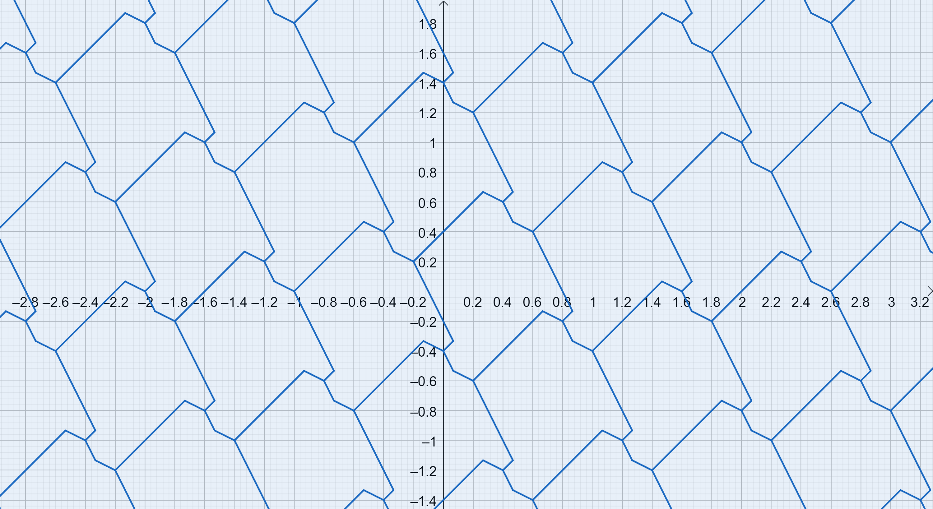
Conjecture 7.5.
For a finite rational irreducible Markov chain, the basin of attraction tiles the hyperplane by translation, and the translation vectors that relate each tile with each other forms an -dimensional sublattice in of with basis vectors .
Proposition 7.6.
For a finite rational irreducible Markov chain, if the basin of attraction tiles the hyperplane with lattice of translation vectors generated by , then the period of any cycle under the hunger game process is the least common denominator of the stationary probabilities of the Markov chain.
Proof.
By using Proposition 7.3, it suffices to show that the tiling condition implies that all periods in the basin of attraction are the same. Suppose the lattice in the statement of the proposition is . We say that two points in are equivalent mod if they differ by an element of , and we write the set of equivalence classes as . Now view the hunger game process, which naturally acts upon , as acting instead on , where the tiling condition implies that the basin of attraction can serve as a set of coset representatives for . Initially this might seem like nonsense since the choice of which state to fire depends on inequalities relating the elements of the hunger vector and these inequalities get washed out when we mod out by , but all rows of are equivalent mod , i.e., each row of has the same image under the projection map , so the choice of which state gets fired is moot; we may as well suppose that the coset is added at each stage, as if state 1 were firing repeatedly. Using the basin of attraction as a set of coset representatives and observing that a vector inside the basin must stay within the basin under the hunger game process, we find the hunger game process on is equivalent to the original hunger game on for any vector in the basin. If the zero vector has period , then in . Then let be the minimum of the set of positive integers such that in . After steps of the hunger game process, every vector in the basin thus returns to itself, so we find and every vector in the basin of attraction must have period , which completes the proof. ∎
We provide a partial result towards 7.5, proving that the basin of attraction translated under the stated lattice covers the hyperplane ; to prove 7.5 and thus 7.4, it remains to show this covering has no overlap.
Proposition 7.7.
For a finite rational irreducible Markov chain, let be the sublattice in of with basis vectors . Then for any vector , there exists a such that lies in the basin of attraction.
Proof.
As is pre-periodic, after some finite number of steps it will reach some vector in the basin, say after steps. Additionally, every vector in the basin stays in the basin under the hunger game process, so for all integers , applying the hunger game process times to yields a vector in the basin. Let be the least common denominator of the stationary probabilities of the unique stationary distribution of our Markov chain, and fix to be the minimum nonnegative integer such that is a multiple of , say for positive integer . Then applying the hunger game process times to yields a vector in the basin of attraction, say after firing state a total of times for each . Constructing vector from these values, as was reached after firing a total of times, we have and . Notice that is the primitive integer vector in the direction of the stationary distribution, so we have . Hence , where . As , letting yields , as desired. ∎
8. Comments
The hunger game achieves high fidelity (that is, low discrepancy) for the frequency with which a specified state occurs, but not for the frequency with which two specified states occur in succession; the rotor-router game achieves fidelity for the frequency with which two specified states occur in succession, but not for the frequency with which three specified states occur in succession. One could use a block-encoding trick (with new states encoding pairs of old states) to construct a simulation scheme that ensures fidelity for the frequency with which three specified (old) states occur in succession, but at a price: the resulting rotor-router network will have more rotors, and hence the quantities that upper-bound discrepancy in [8] will be larger. Indeed, consider derandomization of a fair coin process. De Bruijn [3] showed that for each , there is a cyclic word of length that contains each possible bit-string of length exactly once; it follows that if we let be the infinite word associated with this cyclic word, then for each bit-string of length , the unnormalized discrepancy , defined as minus the number of apperances of in the first positions of , is bounded. On the other hand, one cannot find a single infinite word that accomplishes this task simultaneously for all , since for example if is a string containing one or more 1s, the boundedness of is inconsistent with the occurrence of arbitrarily long strings of 0’s.
We propose that a sort of trade-off principle is at work here: the more numerical characteristics of a random process that we attempt to mimic in a deterministic simulation, the worse our mimicry will be, if our criterion of merit is the rate at which the simulation’s numerical characteristics converge to the limiting values of the corresponding numerical characteristics of the random process. In this context, one sometimes sees the words “psuedorandom” and “quasirandom”, where a pseudorandom simulation is expected to pass “all” tests of randomness while a quasirandom simulation is expected only to pass certain specified tests. It is reasonable to expect that the more asymptotic tests of randomness a quasirandom simulation is required to pass, the worse the convergence will be. Indeed, for certain tests of randomness, the previous assertion is almost a tautology; for if (say) a random sequence of s and s had its running average approach 1/2 with discrepancy smaller than , that rapidity of convergence would ipso facto demonstrate negative correlation between the bits, constituting failure of a correlational test of randomness.
Applying this trade-off principle in the reverse direction, it seems reasonable to hope that by relaxing our stringency, and requiring a quasirandom simulation scheme to pass fewer tests for randomness, we enable it to do a better job with the tests that it is required to pass; that is, we make faster convergence possible. Hence, the delocalized firing mechanism of the hunger game, by no longer preserving the frequency with which two specified states occur in succession, may allow the hunger game to outperform the rotor-router in convergence.
Then under rotor-routing the itinerary of the chip will be periodic with repeating pattern , while under the hunger game the itinerary will simply alternate between 1 and 2, yielding lower discrepancy for the visit-frequencies of the two states.
Acknowledgments
The authors thank Grant Barkley, Darij Grinberg, Sam Hopkins, Lionel Levine, Alex Postnikov, and Tom Roby for various helpful suggestions made during the course of this research. We are grateful to the anonymous referees who made many suggestions that improved this article.
References
- [1] Anders Björner, László Lovász, and Peter W. Shor. Chip-firing games on graphs. European Journal of Combinatorics, 12(4):283–291, 1991.
- [2] Scott Corry and David Perkinson. Divisors and sandpiles. American Mathematical Society, Providence, RI, 2018.
- [3] Nicolaas Govert de Bruijn. A combinatorial problem. Proc. Koninklijke Nederlandse Akademie V. Wetenschappen, 49:758–764, 1946.
- [4] Deepak Dhar. Self-organized critical state of sandpile automation models. Physical Review Letters, 64(23):2837, 1990.
- [5] Arthur Engel. The probabilistic abacus. Educational Studies in Mathematics, 6(1):1–22, 1975.
- [6] Arthur Engel. Why does the probabilistic abacus work? Educational Studies in Mathematics, 7(1-2):59–69, 1976.
- [7] Alexander E. Holroyd, Lionel Levine, Karola Mészáros, Yuyal Peres, James Propp, and David B. Wilson. Chip-firing and rotor-routing on directed graphs. In In and out of equilibrium 2, pages 331–364. Springer, 2008.
- [8] Alexander E. Holroyd and James Propp. Rotor walks and Markov chains. Algorithmic Probability and Combinatorics, 520:105–126, 2010.
- [9] John G. Kemeny and J. Laurie Snell. Finite Markov chains (1983 Edition). Springer-Verlag, 1960.
- [10] Michael Kleber. Goldbug variations. The Mathematical Intelligencer, 27(1):55–63, 2005.
- [11] Caroline J. Klivans. The Mathematics of Chip-firing. Chapman and Hall/CRC, 2018.
- [12] James R. Norris. Markov chains, volume 2 of Cambridge Series in Statistical and Probabilistic Mathematics. Cambridge University Press, 1998.
- [13] Vyatcheslav B. Priezzhev, Deepak Dhar, Abhishek Dhar, and Supriya Krishnamurthy. Eulerian walkers as a model of self-organized criticality. Physical Review Letters, 77(25):5079, 1996.