Factor-of-iid Schreier decorations of lattices in Euclidean spaces ††footnotetext: Mathematics subject classification (2020): 05E18, 05C63, 37A30, 60C05
Abstract
A Schreier decoration is a combinatorial coding of an action of the free group on the vertex set of a -regular graph. We investigate whether a Schreier decoration exists on various countably infinite transitive graphs as a factor of iid.
We show that , the square lattice and also the three other Archimedean lattices of even degree have finitary-factor-of-iid Schreier decorations, and exhibit examples of transitive graphs of arbitrary even degree in which obtaining such a decoration as a factor of iid is impossible.
We also prove that symmetrical planar lattices with all degrees even have a factor of iid balanced orientation, meaning the indegree of every vertex is equal to its outdegree, and demonstrate that the property of having a factor-of-iid balanced orientation is not invariant under quasi-isometry.
1 Introduction
Let be a simple connected -regular graph. A Schreier decoration of is a colouring of the edges with colours together with an orientation such that at every vertex, there is exactly one incoming and one outgoing edge of each colour.
It is a folklore result in combinatorics that every finite -regular graph has a Schreier decoration, and it is easy to extend this to infinite -regular graphs as well. As a generalisation of the finite result, the third author proved in [23] that all -regular unimodular random rooted graphs admit an invariant random Schreier decoration. It is natural to ask whether such an invariant random Schreier decoration can be obtained as a factor of iid. In this article, we investigate this question for some infinite deterministic graphs, more specifically the -dimensional Euclidean grids, symmetrical planar lattices, and graphs quasi-isometric to the bi-infinite path of the form . We study non-amenable graphs in a separate paper [2].
Informally speaking, a Schreier decoration is a factor of iid if it is produced by a certain randomised local algorithm. To start with, each vertex of gets a random label from independently and uniformly. Then it makes a deterministic measurable decision about the Schreier decoration of its incident edges, based on the labelled graph that it sees from itself as a root. Neighbouring vertices must make a consistent decision regarding the edge between them. The factor is finitary if the decision is based only on a finite-radius neighbourhood of each vertex. The precise definition is given in Section 2. Obtaining combinatorial structures or certain models in statistical mechanics as factors of iid is a central topic in ergodic theory. See [15] and the references therein for a recent overview.
A partial result towards a Schreier decoration on a -regular graph is a balanced orientation of the edges. An orientation of the edges of a graph with all degrees even is balanced if the indegree of any vertex is equal to its outdegree. For finite graphs, the term eulerian orientation is often used [19], and when is 4-regular in particular, a balanced orientation is known as an ice configuration in statistical physics [24, 1]. Every Schreier decoration gives a balanced orientation by forgetting the colours.
The main results of the present paper are the following.
Theorem 1.1.
Let be any of the four Archimedean lattices with even degrees (pictured in Figure 1): the square lattice, the triangular lattice, the Kagomé lattice or the lattice. There is a finitary -factor of which is a.s. a Schreier decoration of . Moreover, it has almost surely no infinite monochromatic paths.
Theorem 1.2.
Let denote the -dimensional Euclidean grid. For every , there is a finitary -factor of iid which is a.s. a Schreier decoration of . Moreover, it has almost surely no infinite monochromatic paths.
As far as we are aware, this had not been known, not even in the case of the square lattice. Ray and Spinka show that balanced orientations (under the name “6-vertex-model”) exist on the square lattice as finitary factors of iid [17, Remark 5.3.]. Schreier decorations (that would be the “24-vertex model” in their terminology) are not investigated. In [20], Thornton studies factors of iid which are approximate and exact Cayley diagrams, but his results do not overlap with ours.
Parts of the proof have to be adapted to the individual lattices, but our approach remains the same throughout. We break the lattices into a hierarchy of finite pieces using percolation theory. Then for each piece independently, we choose an edge--colouring scheme such that we can ensure that every monochromatic connected subgraph is a finite cycle. Each cycle will orient itself strongly. We also use a similar hierarchy argument to find balanced orientations on symmetrical planar lattices; see Theorem 3.9.

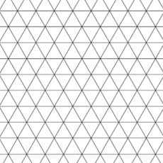


Next we show examples in which it is impossible to obtain a Schreier decoration as a factor of iid.
Theorem 1.3.
For every , there exists a -regular transitive graph that has no factor of iid balanced orientation. In particular, it has no factor of iid Schreier decoration.
Theorem 1.3 answers [21, Problem 3.4]. However, the examples we construct are somewhat unsatisfactory because they are all quasi-isometric to the bi-infinite path . We do not know of any examples of transitive graphs with no factor of iid Schreier decoration that are not quasi-isometric to .
Furthermore, Theorems 1.1 and 1.2 can be phrased in terms of Bernoulli graphings over the respective graphs, yielding the following corollary.
Corollary 1.4.
The Bernoulli graphings of the Archimedean lattices as well as that of admit a probability-measure-preserving action of the free group which satisfies that two vertices of the graphing are adjacent if and only if there is a generator of such that .
This connection is another important motivation for studying factor of iid Schreier decorations because we would like to understand which -regular graphings are so generated by actions of . Our main question can be equivalently formulated as follows: given a (transitive unimodular) -regular graph , is the Bernoulli graphing of generated by a p.m.p. action of ? The connection is spelled out in our parallel paper [2], where we investigate non-amenable graphs and utilise it in the other direction. Our main result there is the following.
Theorem 1.5 ([2]).
Every non-amenable quasi-transitive unimodular -regular graph has a factor of iid that is almost surely a balanced orientation.
For example, all Cayley graphs, in particular regular trees are unimodular. For , the -regular tree is also non-amenable, so it is covered by Theorem 1.5.
The structure of the paper is as follows. In Section 2, we give definitions, present examples for Theorem 1.3, and treat invariance under quasi-isometry. Section 3 is concerned with general planar lattices, breaking them into clusters organised in a hierarchy and obtaining balanced orientations. Building on some of these results, Section 4 gives the proofs of Theorem 1.1 separately for each lattice and of Theorem 1.2. In Section 5, we explore what other combinatorial structures we can obtain using the results and ideas presented thus far. Open questions are collected in Section 6.
Acknowledgement. The authors would like to thank Miklós Abért, Jan Grebík, Matthieu Joseph, Gábor Kun, Gábor Pete, and Václav Rozhoň for inspiring discussions about various parts of this work.
2 Notation and basics
We call a graph transitive if and only if it is vertex-transitive, i.e. the automorphism group acts transitively on the vertex set . We call edge-transitive whenever acts transitively on .
For the rest of the paper, for every , let stand for the -regular -dimensional grid, that is the Cayley graph of with the standard generators after forgetting the labelling. In the planar case, we also use simply in place of .
2.1 Schreier graphs
Given a finitely generated group and an action on some set , the Schreier graph of the action is defined as follows. The set of vertices is , and for every , , we introduce an oriented -labelled edge from to .
Rooted connected Schreier graphs of are in one-to-one correspondence with pointed transitive actions of , which in turn are in one-to-one correspondence with subgroups of . Trivially, a graph with a Schreier decoration is a Schreier graph of the free group on generators. A special case is the (left) Cayley graph of , denoted , which is the Schreier graph of the (left) translation action .
2.2 Factors of iid
Let be a group. A -space is a measurable space with an action . A map between two -spaces is a -factor if it is measurable and -equivariant, that is for every and .
A measure on a -space is invariant if for all and all measurable . We say an action is probability-measure-preserving (p.m.p.) if is a -invariant probability measure.
Let be a graph and . Let denote the Lebesgue measure on . We endow the space with the product measure . The translation action is defined by
The action is p.m.p.
An orientation of can be thought of as a function on sending every edge to one of its endpoints. Viewed like this, orientations of form a measurable function space on which acts. The set of balanced orientations is -invariant and measurable, so it is a -space in itself. Similarly, the set of all Schreier decorations of forms the -space .
Definition 2.1.
A -factor of iid Schreier decoration (respectively, balanced orientation) of a graph is a -factor (respectively, to ). If the group is not specified, we mean an -factor.
Remark 2.2.
We allow to not be defined on a -null subset .
Let us now recall some special classes of iid processes on graphs. For a fixed vertex , let denote the restriction of to the edges incident to . We say is a finitary factor of iid if for almost all , there exists an such that is already determined by . That is, if we change outside , the decoration does not change around . This radius can depend on the particular . If it does not then we say is a block factor.
When constructing factors of iid algorithmically, one often makes use of the fact that a uniform random variable can be decomposed into countably many independent uniform random variables. In practice, this means that we can assume that a vertex has multiple labels or that a new independent random label is always available after a previous one was used.
We will use a reverse operation as well: the composition of countably many uniform random variables is again a uniform random variable. When the number of variables combined is finite, one can do this in a permutation-invariant way. In particular, this allows finite graphs to make joint random decisions as factors of iid by composing the labels of their vertices. So any -invariant random process on a finite graph is a factor of iid. We frequently make use of this on finite subgraphs of our infinite graphs.
For -factors of iid on an infinite transitive graph , the fact that the factor map intertwines the actions of implies that the further two vertices are from each other, the more independently the process behaves around them. We make use of the existence of this correlation decay both later in this section and in Section 6.
2.3 Graphs quasi-isometric to
In this subsection, we present regular graphs of arbitrary even degree with the same large-scale geometry which in one case have factor-of-iid Schreier decorations but in the other not even a factor-of-iid balanced orientation. In both cases, our examples are quasi-isometric to the bi-infinite path , that is the graph with in which and are adjacent if and only if .
For simple graphs and , let the graph be defined by having with vertices and being adjacent if and only if and or and .
Proposition 2.3.
Let be a finite -regular graph with an odd number of vertices. The -regular graph has no -factor of iid balanced orientation.
Proof of Theorem 1.3.
In Proposition 2.3, take to be the -regular clique . As is transitive, so is . ∎
Proof of Proposition 2.3.
First we note that has no -factor of iid balanced orientation. This is because has only two balanced orientations, and so orienting any single edge determines the whole balanced orientation. So two edges at an arbitrary distance get oriented in the same direction with probability . In a factor of iid orientation however, given two edges that are far enough from each other, the probability of them being oriented in the opposite direction is close to .
Second, suppose a balanced orientation of is given. For adjacent vertices , define
and note that .
We also claim that for every . Indeed, as the orientation of is balanced, we have
| (2.1) |
On one hand, oriented edges of of the form contribute 1 to both sides of (2.1). On the other hand, counts the edges of the form contributing to the left-hand side of (2.1), and counts the edges of the form contributing to the right-hand side. Therefore as claimed.
As is odd, we either have or . We now have an argument similar to the one we presented to prove there is no factor of iid balanced orientation of .
Our claim shows that if we have for some , then we have it for all . That is, for , and any random balanced orientation, we have
However, if the balanced orientation of was a factor of iid, for any we could find and far enough such that
Consequently, has no factor of iid balanced orientation. ∎
These non-examples are all quasi-isometric to , which renders them somewhat unsatisfactory (see Question 6.4). Being quasi-isometric to , however, does not imply being a non-example.
Proposition 2.4.
Let be a finite -regular graph which has a perfect matching. Then the -regular graph has an -factor of iid Schreier decoration.
Proof.
Let be a non-empty factor-of-iid 4-independent subset of , that is a subset such that for every , the distance is at least 5. For each , let be a neighbour of in , chosen uniformly at random. Then let both and fix the same perfect matching . Together with the edges between and , these form a 2-factor of (whose all cycles are even).
Next we are going to complement these 2-factors to obtain a 2-factor of the entire . Let , and suppose that are such that but for any . We note that is finite and greater than zero because is a factor of iid and 4-independent, respectively. Now let fix the same perfect matching as does and the same as . Together with the edges of the form , these form a 2-factor of (whose all cycles are even).
Let us give colour to every edge in this 2-factor of and orient each of its finite cycles strongly. Then after removing all the decorated edges, we are left with a -regular graph whose all connected components are finite; in particular, they are all isomorphic to either or a connected component of . To complete the construction, let each connected component pick at random a Schreier decoration with colours . ∎
With a couple more technicalities in the proof, we could in fact tweak the Schreierisation so that all oriented cycles of colour would have length at most and all oriented cycles of the other colours at most . This means that is the Schreier graph of a factor-of-iid action of many more groups than just .
Most -regular graphs with an even number of vertices do have a perfect matching. For example, if they are bipartite or contain a Hamiltonian path, a perfect matching must exist. However, there are instances for every which do not have a perfect matching despite having an even number of vertices [7, 4]. For these, we do not know whether their product with admits a factor-of-iid Schreier decoration and/or a perfect matching; see also subsection 5.1 and Question 6.5.
3 Finite clusters of arbitrary thickness and their hierarchy
In this section, we will develop the main tools to investigate planar lattices. Our main goal is to break the symmetries of the lattice by breaking the lattice into pieces of finite size such that each of the pieces is “wide” enough and surrounded by another one – such a partition will be called a hierarchy. We use percolation theory to obtain a starting hierarchy as a factor of iid process. We also prove that given any starting hierarchy, one can coarsen it in a factor of iid way so that the pieces of the resulting hierarchy have arbitrarily large width. As an application, we show how to obtain a factor of iid balanced orientation of any planar lattice with -fold symmetry and all degrees even.
Throughout this and the following section, for any graph , let denote the usual product measure on , with each coordinate getting the Lebesgue measure.
3.1 General cluster hierarchy and its thickness
To obtain Schreier decorations of three of the Archimedean lattices, we partition their vertex set into finite parts, which we shall call clusters, such that for each cluster , there is a unique cluster surrounding it. That is, a unique part such that is in its convex hull and such that there are adjacent vertices , . Such a partition of can be described by a one-ended infinite tree whose vertices are the finite clusters; are adjacent if and only if one surrounds the other. Moreover, every vertex has a well-defined parent distinguishable from ’s children, should there be any.
Definition 3.1 (Hierarchy).
Let be a graph and a partition of . We say that two distinct parts are adjacent if and only if there is and which are adjacent in . Then is a hierarchy on if the following holds for every .
1) is finite,
2) there is a unique such that and are adjacent and for all but finitely many, any path from to contains a vertex from ,
3) whenever is adjacent to , either or .
Note that it is not necessarily the case that the subgraph of induced by a cluster is connected.
A key feature of the hierarchies we use later is that any two non-adjacent clusters are far from one another. Let us describe how starting with any hierarchy, we can obtain one in which non-adjacent clusters are as far from one another as we wish.
Definition 3.2 (-spaced hierarchy).
Let be a graph and a natural number. A hierarchy on is -spaced if for all non-adjacent , the graph distance is at least .
Proposition 3.3.
Let be a graph and suppose there is a (finitary) -factor of iid hierarchy on . Then , there is a (finitary) -factor of iid -spaced hierarchy on .
Moreover, , there is a (finitary) -factor of iid pair , where is a -spaced hierarchy and is a colouring of the parts with colours such that , if has colour then has colour .
Proof.
Consider the infinite tree whose vertices are the parts of , i.e. the clusters of the hierarchy. Let us now colour uniformly randomly the vertices of green and yellow, independently of each other (in other words, we carry out a site percolation with ). For any vertex , write for the parent of and whenever . Then with probability 1, such that has the opposite colour than . Together with the fact that every vertex is an ancestor of only finitely many other vertices (i.e. ), this means that with probability 1, all monochromatic connected components of the coloured are finite.
For every , let us now merge it with if and only if and have got the same colour or is yellow and is green. The modification this makes on the tree is that of contracting all edges whose two endpoints have the same colour and those edges for which is yellow and is green. This corresponds to coarsening into a new hierarchy which has got the property that for each cluster , the distance is at least 3. This is because every path from to must go through , but consists of at least two clusters of the original hierarchy . More precisely, is the finite union of some former clusters , of and of . surrounds , so there must be unique such that . and being distinct clusters in implies that the vertex was coloured green and yellow. But then cannot be the part of the union through which neighbours , that is , and so .
If we repeat such contraction of the hierarchy tree times to obtain , then for every . However, for such that , we can still have . To fix this, let us divide every to
and define a hierarchy . Then for every such that ,
Two clusters in have got the same parent if and only if they are of the form and for some with . For such a pair, we observe that
Having obtained with whenever are non-adjacent for every , we want to find coloured hierarchies . For fixed , start by considering a hierarchy . Then divide every to parts where
Colouring with colour yields the desired pair . ∎
Remark 3.4.
The Proposition above can be generalised to cases in which siblings are allowed to communicate, i.e. in which two clusters with might be neighbours. This corresponds to modifying the third point in the definition of hierarchy or leaving it out altogether. Under these circumstances, the infinite graph describing the hierarchy is no longer a tree, but a tree-like (or even forest-like) structure with triangles allowed.
3.2 Percolation clusters in planar lattices and their matching lattices
Let be a planar lattice, that is a connected, locally finite plane graph, with a discrete subset of , such that there are translations and through two independent vectors and both of which act on as a graph isomorphism [5]. Note that any planar lattice is necessarily quasi-transitive. We wish to use site percolation in a way that would partition into finite clusters with a hierarchy. For lattices satisfying , i.e. on which site percolation does not occur when , we could colour the vertices uniformly at random yellow and green and consider the monochromatic connected components. However, though this produces, with probability 1, only finite clusters, there isn’t necessarily a clear hierarchy associated to them; this inconvenience is best illustrated by the random vertex 2-colouring of the square lattice. Nevertheless, when the lattice possesses some mild symmetry properties, a two-step solution presents itself. The first step is a result on matching pairs with -fold symmetry.
Definition 3.5 (-fold symmetry, [6]).
For , a plane lattice has -fold symmetry if the rotation about the origin through an angle of maps the plane graph into itself.
Theorem 3.6.
Let be a plane lattice with -fold symmetry for some and its matching lattice, i.e. the graph obtained from by adding all diagonals to all faces of . Then for every , the percolation probabilities , satisfy that or . Furthermore, , where is the Hammersley critical probability.
This result tells us that choosing to randomly 2-colour the vertices of our planar lattice such that a site is yellow with probability and green with probability is well defined. The definition of a cluster hierarchy on then comes naturally, with yellow clusters being exactly the yellow connected components of the random 2-colouring and green clusters the would-be green connected components on (that is in , the green clusters are unions of connected components which have vertices appearing in a same face). The trouble is that the theorem does not guarantee that neither of the colours will have an infinite cluster, or in other words that percolation does not occur at criticality at neither the planar lattice nor its matching lattice. Benjamini and Schramm conjectured in 1996 that this indeed is the case [3]. However, for now, to obtain this crucial property, one needs to analyse lattices one by one (e.g. Russo showed that both critical percolations die for the square lattice and its matching lattice [18]).
The second step in our solution to the hierarchy problem is therefore to add a vertex to every non-triangular face of a lattice with -fold symmetry and connect it to all the vertices of that face. Let us call the resulting lattice and observe that it also has -fold symmetry. is self-matching, and so Theorem 3.6 tells us that and percolation does not occur at criticality.
This finding gives us a factor-of-iid hierarchy on as follows. Colour the vertices of yellow or green uniformly at random. For each non-triangular face, decide uniformly at random whether either all of its yellow vertices will be treated as if they were connected through the face or all of its green vertices will be so treated. This results, with probability one, in a well-defined cluster hierarchy on , which we can combine with Proposition 3.3 to conclude the following.
Theorem 3.7.
Let be a planar lattice with -fold symmetry, . Then for every , there is a finitary -factor of which is almost surely a -spaced hierarchy on .
Theorem 3.7 now allows us to obtain a finitary factor of iid balanced orientation of any planar lattice with -fold symmetry in which all degrees are even. To carry out the construction, we first need to clearly demarcate the clusters.
Definition 3.8 (Boundary ).
Let be a planar lattice and a hierarchy on . The boundary of a cluster is a set of edges with both endpoints in as follows. An edge is in if and only if one of its two contiguous faces consists only of vertices of the cluster and its offspring, while the other contains a vertex from .
Note that in general, it may be the case that , but when all degrees of are even, these two faces must be distinct.
Theorem 3.9.
Let be a planar lattice with -fold symmetry, , in which all degrees are even. There is a finitary -factor of which is a balanced orientation of almost surely.
Proof.
is a discrete set in , i.e. it has no accumulation points, and so there is such that every face of consists of at most vertices. Let us fix a finitary factor of iid -spaced hierarchy on , so that no face contains vertices of non-adjacent clusters, and consider the boundaries , .
We observe that for every vertex , the number of edges from that are incident to is even. Indeed, let be a positive number such that the disc with radius centred on contains no other vertices than , and let be the neighbours of as we traverse them clockwise. Then the edges split into many areas , where moves through clockwise towards (all indices are taken). Now call the faces spanned by ; note that we might have even when . The faces are of two types – those with all vertices from the cluster and its offspring and those with a vertex from . As no face contains vertices of non-adjacent clusters, the edge is in if and only if the two consecutive faces are of different types. But when we start in and make one full circle clockwise back to , the change of types must occur even number of times.
Even though the construction of a spaced hierarchy on based on Proposition 3.3 and Theorem 3.7 does not ensure that all clusters are connected, it does say that is connected (and infinite) for every . Therefore, there is no vertex from inside (each cycle of splits the plane into a finite and an infinite region; by inside, we mean the union of the finite regions). On the other hand, all vertices of any offspring of are inside , so any cluster which has a child must have non-empty boundary. Let us now reassign any vertices of a cluster which are outside to – these are exactly the vertices such that all faces they are in contain a vertex from .
Every cluster will now randomly choose one of two allowed orientation patterns which will be given to all non-boundary edges with at least one endpoint in and none in . These are exactly the edges in the finite region enclosed by , but outside the finite regions enclosed by for all with .
The patterns are as follows: for a vertex and its neighbours , ordered as we traverse them clockwise, we want the orientations of to be alternating between into and out of . In other words, we choose randomly one of the two chessboard colourings of the faces in this region, and orient cycles bounding black faces clockwise and cycles bounding white faces counter-clockwise.
For every cluster , if and happen to choose the same pattern, we will propagate it to as well. If and choose different patterns, then randomly picks one of its balanced orientations (recall that has all degrees even, so a balanced orientation exists).
Finally, we claim that the resulting global orientation of is balanced. If a vertex is not in or if and agree on their patterns, then all the edges incident to follow the same pattern, i.e. they alternate between in and out and the orientation is balanced at . Now suppose and have got different patterns and some of the edges incident to are in . Then let be a disc centred on as before – the boundary edges split it into areas , ordered as we traverse them clockwise, for some integer , where in any pair of adjacent areas, one is inside and one is outside. Inside each area , the number of non-boundary edges is either even or odd. If it is even, half of these edges are oriented towards and half from because they all follow the same pattern. If the number is odd, let be the smallest positive integer such that also contains odd number of non-boundary edges, where is understood mod . If is even then and follow the same pattern and the number of edges between them is even, so exactly half of the edges in is oriented towards and half from . If is odd then and follow different patterns and the number of edges between them is odd, which however also means that exactly half of the edges in is oriented towards and half from . Combined with the fact that due to the balanced orientation of , half of the boundary edges go into and half out of , this means that the orientation at is balanced.
∎
Let us note that the first half of the proof uses neither that the lattice is symmetric nor that all degrees are even, so we can also use it to deduce the following technical lemma that we will heavily use in Section 4.
Lemma 3.10.
Let be a planar lattice and suppose there is a (finitary) -factor of iid which is almost surely a hierarchy on . Then for every , there is a (finitary) -factor of iid which is almost surely a -spaced hierarchy with the additional property that the boundary of any cluster is a union of edge-disjoint cycles and any path between any , must cross . Subsequently, for any distinct clusters , we have that , where is an upper bound on the number of vertices forming any face of .
Proof.
Given , let us fix a -spaced hierarchy (whose existence is ensured by Proposition 3.3), and observe that we can repeat verbatim the proof of that for every vertex , the number of edges from that are incident to is even. It also remains true that for any cluster , the vertices which remained outside of are exactly those such that all faces they are in contain a vertex from . Let us repeat the reassignment of vertices outside to so that for any cluster , as required. In particular, this reassignment leaves the boundaries , intact and ensures the second property.
Finally, if and are distinct non-adjacent clusters then simply because the hierarchy is -spaced. On the other hand, for any and any vertex , the definition of boundary tells us that . But as and do not neighbour, so by the triangle inequality,
Thus as required. ∎
4 Schreier decorations of Archimedean lattices and as finitary factors of iid
An Archimedean lattice is a vertex-transitive tiling of the plane by regular polygons. It is known that there are ten of them (eleven if we count separately the two mirror images of the lattice ; see e.g. [5, Chapter 5]), out of which four have even regularity. These are the infinite grid (that is the Cayley graph of with the standard generators), the triangular lattice (the only 6-regular planar lattice), the Kagomé lattice (i.e. the line graph of the hexagonal lattice ), and the 4-regular lattice where the numbers denote the orders of the faces when we go round a vertex.
4.1 The square lattice
Proof of Theorem 1.1 for .
We start with independent -labels on .
- Step 1
Spaced hierarchy. The square lattice has got 4-fold symmetry, so we can use Theorem 3.7, Proposition 3.3 and Lemma 3.10 to create a -spaced hierarchy based on percolation clusters where is a sufficiently large integer. Moreover, each part is assigned a number from such that every child has got the other number than its parent.
- Step 2
Definition of guards. The guards of an edge are the four of its six incident edges that are perpendicular to it. That is, the four incident edges that appear with in a (see Figure 4).
Figure 4: Each edge has four guards. - Step 3
Red-blue edge colourings inside clusters. Each cluster numbered 1 wants to determine for itself an edge colouring consisting of monochromatic -s. That is, each such cluster finds a vertex (e.g. the one with the largest label) and chooses one of the four -s containing to have all its edges coloured red. As we want our -pattern to be the union of blue -s and red -s and such that every has two incident edges blue and two red, fixing one red determines the rest of the pattern. We call this colouring the inner pattern of .
Figure 5: Examples of what the inner pattern can look like on a fixed 16-vertex square On the other hand, each cluster numbered 2 wants to determine for itself an edge colouring in which all parallel edges have got the same colour (and so every has got two edges red and two blue in an alternating manner, and every edge has different colour than its guards). We call such a colouring an interface pattern.
- Step 4
Amalgamating the patterns. For every cluster numbered 2 (i.e. a cluster with an interface pattern), we will apply its pattern to all edges with at least one endpoint in . Let be a cluster numbered 1 and an edge with both endpoints in . Let be the set of the guards of whose other endpoint (the one not shared with ) is not in (note that might be empty). Then we colour as follows: If there is on which the inner pattern of (should it be extended there) disagrees with the interface pattern by which is coloured, we colour according to the interface pattern, i.e. with the opposite colour than has. This may or may not coincide with the colour the inner pattern would give to . If there is no such guard , is coloured according to the inner pattern of . Our hierarchy being -spaced (where ) ensures that this is well defined.
- Step 5
Claim that the colouring is balanced. In the edge colouring defined above, every vertex has exactly two red and two blue incident edges a.s.
Proof of claim.
If where is numbered 2, then all its four incident edges follow the same interface pattern. As any interface pattern is internally balanced, so are the colours at .
So let us now assume that is in a cluster numbered 1, and consider the 9-vertex square centred on . Regardless of what clusters the remaining 8 vertices belong to, the final colouring of the four edges incident to can be described by saying that we first colour all four of them with the inner pattern (so that a perpendicular pair is red and the complementary one blue), and then recolour if necessary.
First observe that thanks to the hierarchy being -spaced where , the 9-vertex square does not contain both a vertex from and a vertex from a . Hence there is only one interface pattern according to which edges may wish to recolour themselves. Also note that regardless of the inner and the interface pattern, exactly one red and exactly one blue edge out of the four edges incident to already follow the interface pattern at the beginning, so they will not get recoloured in any case. That is, at most two of the four edges will get recoloured.
If two edges get recoloured, then as explained above, one of them is initially blue and one is initially red. So recolouring both of them does not change the multiplicity of colours incident to , and as this multiplicity was balanced to start with, it will remain balanced. If no edges get recoloured, then again, we invoke that the initial colouring was already balanced. Finally, we would like to argue that it cannot happen that exactly one of the four edges gets recoloured.
Let and be the two perpendicular edges on which the inner pattern and the interface pattern disagree, and suppose on the contrary that only gets recoloured. Note that is a guard of , so if then both and would get recoloured. Also is a guard of , so by the same logic we also must have . If , the fourth corner of the square spanned by , and , was not in , then again both and would get recoloured. Finally, the inner pattern and the interface pattern agree on the two remaining guards of , so they will not be recoloured in any case, meaning also does not get recoloured. But that is in contradiction with the assumption that does get recoloured. Hence it cannot happen that exactly one of the four edges incident to gets recoloured.
Figure 6: Vertex has two red and two blue incident edges. ∎
- Step 6
Claim that there are no infinite paths. There are no infinite monochromatic paths in the balanced colouring defined above a.s. That is, the set of blue edges is a union of vertex-disjoint finite blue cycles, and similarly the set of red edges is a union of vertex-disjoint finite red cycles.
Proof of claim.
Suppose there is an infinite monochromatic path . Let be a cluster whose intersection with is non-empty. Then the path must share a vertex with every cluster in the sequence , where and for every positive integer . Pick the such that is numbered 1, and so gets the inner pattern. There must be a section of such that , for every , and for some cluster such that . We used Lemma 3.10 when building the -spaced hierarchy, so we can now deduce that . Moreover, for every and every cluster such that ,
and so . This means that the edges must have empty , and so must all follow the inner pattern of . In particular, as , this is at least four edges. But no monochromatic walk of length four in an inner pattern can contain five distinct vertices (i.e. be a path) because inner patterns are made up of monochromatic -s. This would be a contradiction, and so there is no infinite monochromatic path almost surely. ∎
- Step 7
Orientation. Finally, let each monochromatic cycle choose one of the two strong orientations for itself (e.g. by finding the edge with the largest sum of labels and orienting it from the vertex with the larger label to the one with the smaller label). Then every vertex lies in one strongly oriented blue cycle and one strongly oriented red cycle, and so the coloured orientation is balanced.
∎
Remark 4.1.
In fact, it is not necessary to rely on Proposition 3.3 to prove Theorem 1.1 for . It makes the proof neater, but one can also make do just with the basic percolation clusters for the matching pair . The approach not using Proposition 3.3 (in which every yellow cluster is merged with its green parent into a blob and edges bridging different blobs get an interface pattern) heavily relies on the fact that critical percolation on either of the lattices in this matching pair has no infinite cluster a.s. (though expected sizes of the clusters will be infinite) [18]. Interestingly, the related conjecture of there being no percolation at criticality (site or bond) in has not been settled for (see [11] for a partial progress).
4.2 Grids in higher dimensions
Our construction on made use of the hierarchical structure of clusters, as well as of their thickness preventing local recolourings of edges close to boundaries and other tweaks to overlap. We achieved these desired properties by classical percolation-theoretic results, which are sadly not available in higher dimensions.
However, one could also construct such clusters (arbitrarily spaced) using Borel-combinatorial results of Gao, Jackson, Krohne and Seward [12, 13], as well as of Marks and Unger [16].
In [12] and [13], such hierarchical decompositions named (layered or unlayered) toasts are defined. Theorem 5.5 in [16] (attributed to Gao, Jackson, Krohne, and Seward) states that any Borel action of has a Borel toast of arbitrary thickness. Even though we do not have a action on , the proof in [16, Appendix A] goes through with minor modifications. In fact, one only has to prove [16, Lemma A.2] for up to nullsets, and the rest can be repeated verbatim.
Lemma 4.2 (Factor of iid version of Lemma A.2 from [16]).
For any sequence of integers, there exists a sequence of random subsets of such that is a factor of iid maximal -discrete subset of , and for any and ,
Proof.
Since is transitive, it is sufficient to prove the statement for a fixed vertex.
Let be fixed, and assume that each has countably many iid labels . Let , and define for as follows:
Each set is -discrete, and therefore their increasing union is also -discrete. Moreover, is maximal -discrete with probability 1, because if some could be added to , then it is in with probability , which is bounded away from 0. If could be added to , then an event with probability bounded away from 0 would have to have failed infinitely many times.
Now we argue that , where is a constant independent of . Indeed, with probability , the maximum of within is obtained somewhere within , and therefore , which also implies . Thanks to the polynomial growth of , the ratio is bounded away from 0 by a constant independent of .
Generating independently of each other using the above construction with , we get the desired sequence of subsets. The set of indices where is infinite because each is in it independently with probability at least . ∎
The constructed above are in fact finitary factors. The rest of the proof of [16, Theorem 5.5] implies the following.
Corollary 4.3.
admits a finitary factor of iid -spaced hierarchy for any .
While we were writing this paper up, Jan Grebík and Václav Rozhoň informed us that using techniques developed in [8], they can prove the existence of (Borel) toasts in any Borel graph with connected components isomorphic to . This should allow one to construct Borel Schreier decorations on all such Borel graphs [14].
Proof of Theorem 1.2.
We will first construct a balanced edge colouring with colours , and then give orientation separately to each monochromatic cycle.
- Step 1
- Step 2
Edge colouring of even-numbered clusters. The edges of travel in different directions. Let us observe that if we remove all edges in of them, we are left with disjoint copies of the square lattice. Each cluster such that is odd will be assigned an interface pattern in direct analogy to subsection 4.1. By an interface pattern, we understand a balanced edge colouring in which the edge directions of and the colours are in bijection. That is, after removing all edges of any directions (= all edges of any colours), we would end up with an interface pattern on disjoint copies of the square lattice.
In particular, each cluster numbered identifies its ancestor (which is also numbered ) and then all its -th generation offspring . The clusters will make a common choice of the interface pattern.
Subsequently, each -numbered cluster identifies its nearest -numbered ancestor and should there be any, also its nearest -numbered offspring and their interface patterns. The role of the -numbered clusters, as well as of the odd-numbered clusters, is to provide a balanced transition between the patterns of the -numbered clusters.
If a -numbered cluster has no -numbered offspring then it will simply copy the pattern from . Otherwise, we will assign interface patters so that for any cluster with , the directions of the colours in and agree. In particular, we will first assign patterns to 2-numbered clusters, then 4-numbered etc. all the way up to . A -numbered cluster shall identify the interface patterns of its grandchildren and of . If these agree in the direction of the colour then will simply adopt the pattern of its grandchildren without a change. If they disagree then will employ the interface pattern obtained from that of its grandchildren by swapping and the colour that currently travels in the direction that takes in .
- Step 3
Edge colouring of odd-numbered clusters. Each cluster such that is odd will be assigned an inner pattern. By an inner pattern, we understand a balanced edge -colouring in which all the edges in chosen directions have the same colour, while the remaining copies of the square lattice get a pattern consisting of monochromatic -s of the remaining two colours (that is an inner pattern in the sense of subsection 4.1).
In particular, each odd-numbered cluster identifies its parent and its interface pattern and its children (should there be any) and their interface pattern. By construction, these two interface patterns are either the same or one can be obtained from the other by a single transposition, that is by swapping two colours. In the former case and also when has no children, will randomly choose two colours and put monochromatic -s to the grids spanned by their two directions. In the latter case, the -s shall be built from the two colours on which the two interface patterns disagree. Anyhow, the colours and directions of the colours not chosen to form -s will propagate through without change of direction.
- Step 4
Boundaries between clusters. Whenever two clusters and meet, there are colours which simply travel in a fixed direction, which is moreover the same in and . We will let these colours propagate in their directions also on all edges with one endpoint in and one in . After disregarding these, we are left with copies of the square grid, and on every such copy, we see an inner pattern in the sense of subsection 4.1 coming from one of the clusters and interface pattern from the other one. We amalgamate these into a balanced colouring as in subsection 4.1.
Finally, we observe that for every and , there is, with probability 1, an such that has an inner pattern and one of the colours of its -s is . Therefore, there cannot be any infinite monochromatic path, and every colour class is almost surely a union of finite cycles. To finish the construction, let each monochromatic cycle randomly choose one of the two strong orientations for itself.
∎
4.3 The triangular lattice
Similarly as in the case of the higher-dimensional grids, once we have a spaced enough hierarchy, we can use the patterns developed for to obtain a Schreier decoration of .
Proof of Theorem 1.1 for .
We will first construct a red-blue-green edge colouring and then as in the previous case, give orientation separately to each monochromatic cycle.
- Step 1
Spaced hierarchy. has got 3-fold symmetry and is self-matching, so Theorem 3.6 tells us that its site-percolation critical probability is and percolation does not occur at criticality. Let be the finitary factor of iid hierarchy on given by the percolation clusters, and let us use Proposition 3.3 to obtain from it where is a sufficiently large integer and is a -spaced hierarchy.
- Step 2
Edge colouring of odd-numbered clusters. The edges of travel in three different directions. Let us observe that if we remove all edges in one of them, we are left with the square lattice. Each cluster numbered 1 or 3 will be assigned an inner pattern. By an inner pattern, we understand a balanced edge 3-colouring in which all the edges in a chosen direction have the same colour, while the remaining square lattice gets a pattern consisting of monochromatic -s of the remaining two colours (that is an inner pattern in the sense of subsection 4.1). In particular, each cluster numbered 1 identifies its grandparent (which is numbered 3) and then all its grandchildren . The clusters will make a common choice of the inner pattern. They randomly choose one of the three edge directions, colour all edges in the chosen direction green, and put blue and red -s on the remaining square lattice.
Subsequently, each cluster numbered 3 identifies its grandchildren (should there be any) and their inner pattern and its grandparent and its inner pattern. Then it chooses the direction not chosen by either of the patterns and colours all its edges blue. If there is a choice between two directions, siblings (i.e. clusters with the same parent ) make it together.
Every odd-numbered cluster will apply its chosen inner pattern to all edges which are inside , but outside the boundaries of its children.
- Step 3
Edge colouring of even-numbered clusters. Each cluster numbered 2 or 4 will be assigned an interface pattern in direct analogy to subsection 4.1. By an interface pattern, we understand a balanced edge colouring in which the edge directions of and the three colours are in bijection. That is, after removing all edges of any of the directions (= all edges of any of the colours), we would end up with an interface pattern on the square lattice.
In particular, each even-numbered cluster identifies its parent and its inner pattern and its children (should there be any) and their inner pattern. By construction, these two inner patterns disagree both in their chosen direction and their chosen colour. To the direction of , will assign the colour chosen by (i.e. green if is numbered 1 and blue if it is numbered 3). To the direction of the pattern of its children, will assign the colour chosen by the children. This fully determines the interface pattern of (if has no children, then it shall randomly choose one of the two suitable patterns).
(a) An example of an inner pattern (b) An example of an interface pattern Figure 7: Examples of patterns used in odd- and even-numbered clusters - Step 4
Boundaries. Let , be the cluster boundaries as per the definition in subsection 3.2. For every , we want the boundary between and to travel only in the two directions not chosen by the odd-numbered cluster. Suppose that travels in the undesired direction and are the common neighbours of and . Then by the definition of a boundary, exactly one of is in and one is in (without loss of generality, ). We will replace every such in the boundary with the pair . As is -spaced and , such changes cannot cause that boundaries of two different clusters would touch (share a vertex).
Now for a cluster , there is exactly one colour such that there is a direction in which all the edges of both and have colour . Moreover, the boundary never travels in this direction, so after forgetting the edges of colour , we are left with two neighbouring clusters in the square lattice, one of which has got the inner pattern and the other the interface pattern. We proved in subsection 4.1 that there is a 2-colouring of the boundary which amalgamates the two patterns into a balanced 2-colouring.
Finally, as in subsection 4.1, there are no infinite monochromatic paths a.s. To finish the construction, let each monochromatic cycle randomly choose one of the two strong orientations for itself.
∎
4.4 The Kagomé and the lattice
The remaining two Archimedean lattices differ from the first two ones in that not all faces are bounded by cycles of the same length (the lattice is not even edge-transitive). This slightly increased heterogeneity makes the proofs much easier, and in the latter case we even obtain an upper bound on the length of monochromatic cycles, meaning the resulting decoration is a Schreier graph of actions of many more groups than just .
Proof of Theorem 1.1 for .
Split the lattice into finite clusters organised in a hierarchy as in Lemma 3.10. Each finite cluster picks a pattern composed of monochromatic (red and blue) triangles. There are two ways to randomly place this pattern on the Kagomé lattice. Consider the boundaries where . If a boundary travels on two out of the three edges of a given triangle , replace the two edges in the boundary (say ) by the third one () – as a side effect, each boundary becomes a union of vertex-disjoint cycles.
Let each cluster apply its pattern to all non-boundary edges with at least one endpoint in . If two neighbouring clusters and agree in their pattern, simply propagate it to as well. If and disagree, we will colour the boundary as follows. Suppose is in and is the common neighbour of and . Then by construction, either all three edges are in the boundary (in which case we will propagate the pattern of to them) or neither nor is in the boundary. In the latter case, and follow the same pattern and are in the same triangle, so they are assigned the same colour. Let get the opposite colour.
As remarked earlier, every vertex is incident to either two or none edges from . If it is incident to none and also if the patterns of and agree, the colouring at is an inner pattern, which is balanced. If is incident to two boundary edges and and , the same reasoning applies. Finally, if the patterns disagree and and are not adjacent, let be the common neighbour of and and the common neighbour of and . Then has the opposite colour than by the definition of the colouring on boundaries, and similarly has the opposite colour than . Hence the amalgamated colouring is balanced at every vertex.
As in the previous cases, the colour classes are thus unions of finite cycles, and we let each monochromatic cycle randomly pick one of the two possible strong orientations to finish the decoration. ∎
Proof of Theorem 1.1 for .
The lattice is not edge-transitive which makes constructing a Schreier decoration easy in this case. Every edge is either part of a triangle or a hexagon, but not both.
Therefore, we can simply colour all triangles red and all hexagons blue. To complete the Schreier decoration, we choose a random strong orientation for each triangle and hexagon independently. ∎
Constructing a factor of iid perfect matching on the lattice is similarly easy: each hexagon can choose one of its two perfect matchings independently at random, and these matchings together form a perfect matching of the whole lattice.
5 Ramifications for proper edge colourings and perfect matchings
Proper edge -colourings encode actions of the group , the -fold free product of with itself, just like Schreier decorations encode actions of the free group . Both groups have as their standard Cayley graph, and is the universal cover of any -regular graph. In this sense, looking for these structures on -regular graphs is equally natural, but we focus more on Schreier decorations because all -regular graphs have a (deterministic) Schreier decoration, while this is not the case for proper edge -colourings. When searching for these structures as factors of iid, however, we do not know of a single transitive example, where one exists and the other does not.
5.1 Proper edge -colourings and perfect matchings
The absence of infinite monochromatic paths in our Schreier decorations allows us to immediately obtain proper edge -colourings whenever the graph in question is bipartite.
Corollary 5.1 (of Theorems 1.1 and 1.2).
For every , there is a finitary -factor of iid which is a proper edge -colouring of almost surely. Subsequently, there is a finitary -factor of iid which is a perfect matching of almost surely [22].
Proof.
The factors from Theorems 1.1 and 1.2 partition the edges of into finite monochromatic cycles. is bipartite, so all of these cycles are even. To obtain a proper -colouring, let each cycle of colour choose randomly one of the two proper 2-colourings of its edges by and .
By choosing one colour class (say ), we obtain the second statement. ∎
In fact, one can now obtain many more corollaries simply by noticing when graphs have got a decomposition into several locally identifiable copies of . The square lattice with diagonals added is an example of a transitive graph that decomposes into three copies of the square lattice.
Corollary 5.2.
There is an -factor of which is a Schreier decoration a.s. Moreover, it has almost surely no infinite monochromatic paths. Subsequently, there is an -factor of which is a perfect matching of a.s.
If care is taken while constructing a Schreier decoration, bipartiteness is, however, not necessary not even when is not made up of -s.
Corollary 5.3 (of Proposition 2.4).
Let be a finite -regular graph whose chromatic index is . Then there is a finitary -factor of iid which is a proper edge -colouring of almost surely.
Proof.
Let us in the proof of Proposition 2.4 always choose a matching which is given by a colour class of a proper edge colouring. We made sure in the proof to spell out that all cycles of colour have even length. On each of those, pick randomly one of the two proper edge colourings with colours and .
Now on each connected component left after removing the decorated edges which is isomorphic to , pick randomly a proper edge colouring with colours . On each component isomorphic to , let the edges between and all have colour , while we properly colour both and with . ∎
We can again obtain a perfect matching of by choosing one of the colour classes, but there is already the trivial construction of simply picking a perfect matching on each of the copies of .
5.2 Line graphs
Proposition 5.4.
Let be a -regular graph. Then if admits a factor-of-iid Schreier decoration, so does its line graph .
Proof.
If then , so the statement is a tautology.
If then there is a 1-to-1 correspondence between vertices of and the cliques in . Also every vertex in is in exactly two cliques because it has two endpoints in .
Suppose now that is isomorphic to and its vertices are . Let us fix a proper edge -colouring of with colours . Then put on top an orientation such that for all , the edge of colour incident to is oriented towards if and only if the edge of colour incident to is oriented from . This decorated will serve as a template for decorating the cliques of .
Indeed, the Schreier decoration of gives rise to a vertex -colouring of with colours such that moreover, every vertex of labels one of the cliques it is in as ‘in’ and the other as ‘out’. Also every clique in has vertices which are relatively to this clique labelled . Given this vertex decoration, let every in decorate its edges as dictated by the template . Since every is in its other clique, this gives a Schreier decoration of . ∎
Interestingly, we cannot use the same strategy to show that a proper edge -colouring of implies a proper edge -colouring of . This is exactly because every vertex of the line graph would get a decoration which is the same as viewed from either of the two cliques is in. However, when is even, we get the following.
Proposition 5.5.
Let be a -regular graph where is an even positive integer. Then if admits a factor-of-iid balanced orientation, its line graph has a factor-of-iid perfect matching.
Proof.
Every vertex of gives rise to in with vertices labelled ‘in’ and labelled ‘out’. As is even, in each such clique, we can pick a (random) perfect matching on the vertices labelled ‘in’ – crucially, these are labelled ‘out’ with respect to the other cliques they are in. We claim that this is a perfect matching. Similarly as before, the balanced orientation of gives a vertex decoration of such that every vertex is labelled exactly once with ‘in’ and once with ‘out’, therefore at every vertex, there is exactly one matched edge to be chosen. ∎
6 Open questions and remarks
Question 6.1.
Is it true that for all -regular graphs which are vertex- or edge-transitive, the following are equivalent?
- 1.
There is a factor of iid which is a proper edge -colouring of a.s.
- 2.
There is a factor of iid which is a perfect matching of a.s.
- 3.
There is a factor of iid which is a Schreier decoration of a.s.
- 4.
There is a factor of iid which is a balanced orientation of a.s.
We have demonstrated in this paper that all four of the structures exist as factors of iid for , for where is a finite -regular graph with , and more loosely speaking for graphs that are made up of locally identifiable copies of these. We have also constructed Schreier decorations and balanced orientations on more planar lattices than and believe that the hierarchies which are available on them should make it possible to obtain proper edge -colourings too. Also pointing in this direction is the fact that all amenable Cayley graphs have got invariant random perfect matchings [9, 10] – the lattices and are indeed Cayley graphs of and respectively.
On the other hand, where is odd forms the prominent example of a class of graphs where none of the four factors exist. We have shown in Proposition 2.3 that no balanced orientation of is a factor of iid, and the proof that there is no factor-of-iid perfect matching follows similar lines. Indeed, suppose a perfect matching of is given, and let be the number of edges in of the form . Then for every , if is odd then must be even and if is even then must be odd. This is, however, in contradiction with the existence correlation decay in factor of iid processes.
In our parallel paper [2, Definition 22], we further show a class of -regular bipartite graphs for which a proper edge -colouring exists as a factor of iid if and only if perfect matching does if and only if Schreier decoration does. All the above leads us to tentatively conjecture that the answer to Question 6.1 is yes for amenable graphs.
It also seems that if the transitivity assumption is relaxed, the four structures are listed in a strictly decreasing order of difficulty. As we said, where is odd has not got a factor-of-iid balanced orientation, which by [2, Lemma 25] means has no factor-of-iid perfect matching. Thus has no factor-of-iid edge -colouring either by [2, Proposition 5]. The non-transitivity of , however, allows for locally recognisable factorisation of the graph into copies of , which implies the existence of factor-of-iid balanced orientation whenever is even.
To get graphs with a factor-of-iid Schreier decoration but without a factor-of-iid perfect matching, we can start with any -regular satisfying Question 6.1 in its positive sense and by attaching two pendant to every vertex obtain a -regular graph which has no perfect matching at all. Alternatively, we can construct graphs like the one in Figure 9 which have deterministic, but not factor-of-iid perfect matchings. Any perfect matching contains two or no edges of the big squares in an alternating fashion, which again violates correlation decay. However, Schreier decoration can be constructed by colouring the two edges to the left of a cut vertex red and to the right blue, or vice versa, chosen randomly and independently at each cut vertex. Each remaining finite component properly extends this 2-colouring and monochromatic cycles get a random strong orientation.
Finally, any finite -regular graph has a factor-of-iid Schreier decoration, so whenever its chromatic index equals , we again get an example in which a proper edge -colouring does not exist, but when a perfect matching does, like in the Meredith graph, we get an instance for the last type which has exactly three of the four structures as factors of iid.
Question 6.2.
Is there a -regular quasi-transitive graph which has a factor-of-iid proper edge -colouring or perfect matching, but not a factor-of-iid Schreier decoration or balanced orientation?
We also point out that all the Schreier decorations constructed in this paper have no infinite monochromatic paths, i.e. no infinite orbits.
Question 6.3.
Is there a factor of iid Schreier decoration on the square lattice that has infinite monochromatic paths with positive probability? Or on any of the other lattices we consider? Or on any transitive graph?
By ergodicity, this would imply that the factor of iid Schreier decoration has infinite monochromatic paths with probability 1. The next question aims to improve our counterexamples.
Question 6.4.
Give an example of a transitive graph that is not quasi-isometric to and has no factor of iid balanced orientation. Or has no factor of iid Schreier decoration.
In fact, the best would be to have a precise structural description of when these decorations exist as factors of iid.
Question 6.5.
Give a necessary and sufficient condition for a -regular transitive graph to have a factor of iid balanced orientation and/or Schreier decoration.
References
- [1] R. J. Baxter. Exactly Solved Models in Statistical Mechanics. Academic Press, London, 1982.
- [2] Ferenc Bencs, Aranka Hrušková, and Lászlo Márton Tóth. Factor-of-iid balanced orientation of non-amenable graphs. preprint, 2021.
- [3] Itai Benjamini and Oded Schramm. Percolation beyond , many questions and a few answers. Electronic Communications in Probability, pages 71–82, 1996.
- [4] Zoltán L. Blázsik, Jay Cummings, and Willem H. Haemers. Cospectral regular graphs with and without a perfect matching. Discrete Mathematics, 338(3):199–201, 2015.
- [5] Béla Bollobás and Oliver Riordan. Percolation. Cambridge University Press, 2006.
- [6] Béla Bollobás and Oliver Riordan. Percolation on dual lattices with -fold symmetry. Random Structures & Algorithms, 32(4):463–472, 2008.
- [7] Carlos Carbonera and Jason Shepherd. On the existence of a perfect matching for 4-regular graphs derived from quadrilateral meshes. SCI Institute. 04 2006.
- [8] Clinton Conley, Steve Jackson, Andrew Marks, Brandon Seward, and Robin Tucker-Drob. Borel asymptotic dimension and hyperfinite equivalence relations. preprint arXiv:2009.06721, 2020.
- [9] T. Conley, A. Kechris, and R. Tucker-Drob. Ultraproducts of measure preserving actions and graph combinatorics. Ergodic Theory and Dynamical Systems, 33:334–374, 2013.
- [10] Endre Csóka and Gábor Lippner. Invariant random perfect matchings in Cayley graphs. Groups, Geometry, and Dynamics, 11(1):211–244, 2017.
- [11] Michael Damron, Charles M Newman, and Vladas Sidoravicius. Absence of site percolation at criticality in . Random Structures & Algorithms, 47(2):328–340, 2015.
- [12] Su Gao, Steve Jackson, Edward Krohne, and Brandon Seward. Forcing constructions and countable Borel equivalence relations. preprint arXiv:1503.07822, 2015.
- [13] Su Gao, Steve Jackson, Edward Krohne, and Brandon Seward. Continuous combinatorics of abelian group actions. preprint arXiv:1803.03872, 2018.
- [14] Jan Grebík and Václav Rozhoň. Of Toasts and Tails. preprint arXiv:2103.08394, 2021.
- [15] Russell Lyons. Factors of IID on trees. Combinatorics, Probability & Computing, 26(2):285, 2017.
- [16] Andrew S Marks and Spencer T Unger. Borel circle squaring. Annals of Mathematics, pages 581–605, 2017.
- [17] Gourab Ray and Yinon Spinka. Finitary codings for gradient models and a new graphical representation for the six-vertex model. preprint arXiv:1908.09056, 2019.
- [18] Lucio Russo. On the critical percolation probabilities. Zeitschrift für Wahrscheinlichkeitstheorie und verwandte Gebiete, 56(2):229–237, 1981.
- [19] Alexander Schrijver. Bounds on the number of Eulerian orientations. Combinatorica, 3(3-4):375–380, 1983.
- [20] Riley Thornton. Factor Maps for Automorphism Groups via Cayley Diagrams. preprint arXiv:2011.14604v2, 2021.
- [21] Riley Thornton. Orienting Borel graphs. preprint arXiv:2001.01319v2, 2021.
- [22] Ádám Timár. Invariant matchings of exponential tail on coin flips in . preprint arXiv:0909.1090, 2009.
- [23] László Márton Tóth. Invariant Schreier decorations of unimodular random networks. preprint arXiv:1906.03137, 2019.
- [24] D. J. A. Welsh. The computational complexity of some classical problems from statistical physics. Disorder in Physical Systems, 1990.
Ferenc Bencs
Alfréd Rényi Institute of Mathematics, Budapest, Hungary
bencs.ferenc@renyi.mta.hu
Aranka Hrušková
Central European University, Budapest, Hungary
aranka@renyi.mta.hu
László Márton Tóth
École Polytechnique Fédérale de Lausanne, Switzerland
laszlomarton.toth@epfl.ch