Structural Interventions in Networks Thanks: For useful comments and suggestions we thank Nizar Allouch, Francis Bloch, Yann Bramoulle, Antonio Cabrales, George Charlson, Hanming Fang, Itay Fainmesser, Ben Golub, Sanjeev Goyal, Matthew Jackson, Ernest Liu, Evan Sadler, Adam Szeidl, Fernando Vega-Redondo, Yves Zenou, and participants at conferences and workshops.
Abstract
Two types of interventions are commonly implemented in networks:
characteristic intervention, which influences individuals’ intrinsic incentives, and structural intervention,
which targets the social links among individuals.
In this paper we provide a general framework to evaluate the distinct equilibrium effects of
both types of interventions. We identify a hidden equivalence between a
structural intervention and an endogenously determined characteristic
intervention. Compared with existing approaches in the literature, the
perspective from such an equivalence provides several advantages
in the analysis of interventions that target network
structure. We present a wide range of applications of our theory, including
identifying the most wanted criminal(s) in delinquent networks and targeting
the key connector for isolated communities.
JEL Classification: D21; D29; D82.
Keywords: Network games; Structural intervention;
Katz-Bonacich centrality; Targeting;
1 Introduction
Social ties shape economic agents’ decisions in a connected world, ranging from which product to buy for consumers, how much time to spend studying for pupils, how much effort to exert for workers on a team, whether to commit a crime for teenagers, etc.11 1 Numerous studies have highlighted the influence of networks in different contexts such as microfinance (Banerjee et al. 2013); firm performance (Cai and Szeidl 2018); productivity at work (Mas and Moretti 2009); R&D (Goyal and Moraga-González 2001); education (Sacerdote 2001; Calvó-Armengol et al. 2009); crime (Ballester et al. 2006); public goods provision (Bramoullé and Kranton 2007; Allouch 2017); brand choice (David and Dina 2004); and policy intervention Galeotti et al. 2020). For recent surveys, see, for instance, Bramoullé et al. 2016; Jackson et al. 2017; Elliott et al. 2019. These social ties, structurally represented as a network, govern individual incentives and therefore collectively determine equilibrium outcomes and welfare in the society. Thus, structural intervention in social ties provides an important policy instrument for the social planner. A natural research question arises: how to best intervene in the social structure to maximize a certain performance objective subject to certain resource constraints. This research problem is inherently difficult, as it is well known that networks operate in a complex manner. Local changes in social links between a few nodes can influence the actions of a large set of nodes, including those that are far away through ripple effects. Furthermore, the influence is not homogeneous: Nodes that are closer to (further away from) the origin of shocks tend to be more (less) responsive. These key features of shock propagation and heterogeneous responses make the analysis of structural interventions both intriguing and challenging.22 2 Admittedly, these two features are also true for other types of intervention, such as the characteristic intervention. As shown in Section 2.2, the problem of characteristic intervention in a fixed network is much simpler and has been extensively studied in the literature.
In this paper, we propose a general yet tractable framework to quantitatively assess the consequences of an arbitrary structural intervention in social ties on equilibrium actions. By overcoming the challenges described above, we present a neat characterization result in Proposition 1 that evaluates the change in equilibrium behavior in response to changes in the network structure. We then apply Proposition 1 to several economic settings, such as key group removal in delinquent networks (in Section 3) and key connectors for isolated communities (in Section 4).
More specifically, our model of structural intervention builds on a seminal paper by Ballester et al. 2006 (BCZ hereafter), who propose a simple yet powerful model of interactions in a fixed network.33 3 The model in BCZ has been applied, empirically tested, and generalized extensively in the network literature; see, for example, Calvó-Armengol et al. 2009; Chen et al. 2018b; Galeotti et al. 2020. They identify the equivalence between equilibrium actions in a network game and the Katz-Bonacich centralities in sociology (Bonacich 1987). The Katz-Bonacich centrality of a node on a network simply counts the sum of geometrically discounted walks originating from this node to all other nodes in the network, weighted by the characteristics of the ending nodes.44 4 This Katz-Bonacich centrality (and its variants and generalizations) plays important roles in shaping agents’ decisions in a wide range of network models; see, for instance, production networks (Acemoglu et al. 2012; Baqaee 2018; Liu 2019) and the pricing of social products (Candogan et al. 2012; Bloch and Quérou 2013; Chen et al. 2018a). Proposition 1 in our paper characterizes the impacts of structural intervention on the equilibrium by employing another equivalence result: Any (local) intervention on the network structure is equivalent to a (local) endogenously determined intervention on characteristics. Specifically, we find that the equilibrium induced by a structural intervention coincides with that induced by an endogenously determined characteristic intervention without changing the network structure. Moreover, the endogenously determined characteristic intervention only changes the characteristics of the players whose social ties are altered by the structural intervention. The analysis of post-intervention equilibrium becomes much simpler after translating a structural intervention to the characteristic intervention, since the latter changes an individual’s equilibrium behavior linearly and is well studied in the literature, while the former is nonlinear. Furthermore, in Corollary 1, we provide a sufficient condition on a structural intervention to induce higher aggregate equilibrium activity, and use it to check the effect of a link reallocation or a link swap on the aggregate action.
For applications, we first adopt the outcome equivalence result to study the key group problem, which aims to specify the group of players, that if removed, reduces the aggregate equilibrium activity the most. Specifically, the removal of a group of players is equivalent to a certain characteristic intervention restricted to this group. Such a characteristic intervention is chosen to ensure that within the original network, the induced equilibrium efforts of nodes in this group reduce to zero. As a generalization of the single node intercentrality given by BCZ, we provide a closed-form index of group inter-centrality explicitly. Such an index takes into account both the activities nodes in this group and their influences on nodes outside the group. The group intercentrality index reveals that the higher the connectedness between nodes within a group, the lower the intercentrality of the group. Therefore, the greedy algorithm, which sequentially selects nodes with the highest single node intercentrality, may fail to find the key group with the highest intercentrality. We also show that the group intercentrality index is equivalent to the aggregate sum of all walks that must pass the group. As a by-product, we characterize the aggregate sum of all walks starting from one group and ending at the second group, which does not pass the third group. This result generalizes some of the findings on the targeting centrality proposed by Bramoullé and Genicot 2018 in an information diffusion setting.
Next, we introduce a bridge index to characterize the impact of building a bridge between separated networks (Proposition 4). We use the bridge index to fully solve the key bridge problem. Furthermore, we show that the key bridge player must locate at the Pareto frontier of Katz-Bonacich centrality and self-loop in the network. In general, the selection of a bridge pair is an interdependent decision across two networks, since the identity of a key bridge player in one network depends on who is selected as his partner in the second network. These findings are summarized in Corollary 2 and illustrated in Example 3. We also extend the analysis to consider the value of an existing link (the key link problem) and the value of a potential link for an arbitrary network in Section 4.2. As an illustration, we compare intergroup links and intragroup links in Example 4.
Our paper builds on the vast literature on network games (see Ballester et al. 2006; Bramoullé and Kranton 2007; and Galeotti and Goyal 2010). These papers typically characterize the effects of network structure on equilibrium behavior. Our paper instead focuses on how interventions on network structures affect equilibrium outcomes and sheds light on policy design that targets at network structure.
The literature on interventions in networks can be broadly divided into two categories: characteristic intervention and network structure intervention. In the first category, the characteristics of individuals can be changed by subsidy or taxation on choices. For instance, Demange 2017 and Galeotti et al. 2020 study the optimal intervention on characteristics subject to a fixed budget constraint and a quadratic adjustment cost, respectively. Motivated by Ballester et al. 2006; Ballester et al. 2010, our paper mainly focuses on the second category: structural intervention. The identified equivalence between a structural intervention and an endogenously determined characteristic intervention in our paper provides an interesting link between these two categories. Several papers on network formation study the most efficient network by analyzing the impact of link shifting (e.g., Belhaj et al. 2016 and Li 2020). As a complementary result, we propose a sufficient condition to guarantee that a structural intervention leads to higher aggregate action.
An important topic in social networks is the relative importance of a node in a given network using diverse indices. Various centrality measures have been proposed to serve the purpose. Bloch et al. 2020 take an axiomatic approach to provide a unified perspective on several commonly used centrality measures. Ballester et al. 2006 give a micro-foundation of Katz-Bonacich centrality and propose another measure – i.e., intercentrality – to characterize the impact of a node removal. Analogous measures for a group of nodes, instead of a single node, are not fully developed. One exception is Ballester et al. 2010, who define group intercentrality. One of our contributions is proposing a specific form of group intercentrality using the statistics in the underlying network; we show that group intercentrality decreases with connectedness between group members. Bramoullé and Genicot 2018 study the contribution of a pair of nodes (one sender and one receiver) in an information transmission setting. Our analysis in Section 3.2 can be viewed as an extension of their results by allowing multiple senders and multiple receivers.
This paper also speaks to the literature on the effect of bridge(s) between isolated communities. Cai and Szeidl 2018 demonstrate that business meetings facilitate interfirm communications and create enormous economic value by increasing firm performance. To the best of our knowledge, Golub and Lever 2010 is the only network paper to theoretically study the impact of bridge. They consider a social learning model, and their main focus is on the eigenvalue centrality. Our paper, instead, studies the impact of a bridge on Katz-Bonacich centralities and proposes an explicit bridge index to characterize the key pair of nodes connecting two separated networks. See Golub and Lever 2010 for a comprehensive discussion of the related literature.
2 Interventions in networks: Theory
2.1 Setup
Baseline game played on a network Consider a network game played by a set of players embedded in a social network , which is represented by an adjacency matrix . Each player chooses an effort simultaneously with payoff function given as follows:55 5 In Section 5, we discuss several extensions of the baseline model.
| (1) |
This specification of payoff closely follows from Ballester et al. 2006, where measures player ’s intrinsic marginal utility (hence ’s characteristic), denotes player ’s cost of effort, and the last term, , captures the interaction term that represents local network effects among players. The scalar parameter controls the strength of network interaction. We assume so the game exhibits strategic complementarity. We use to denote the network game represented above, where is the characteristics vector.
Throughout the paper, we impose the standard assumptions that (i) is symmetric with , and (ii) for all .66 6 For ease of interpretation, we focus on undirected zero-one network matrix . Our results can be easily generalized to weighted directed networks. Let denote the spectral radius of matrix . By Perron-Frobenius theorem, also equals the largest eigenvalue of . The following is a well-known measure of centralities in network literature.
Definition 1.
Given a network , a scalar , and an -dimensional vector , we define -weighted Katz-Bonacich centralities as
| (2) |
provided that . When , we call the unweighted Katz-Bonacich centralities. Define the Leontief inverse matrix
| (3) |
so that .
Intuitively, counts the total number of walks from to in network with path of length discounted by . So ’s Katz-Bonacich centrality is the sum of walks starting from and ending at any node with weights .77 7 This follows from the following identity of the Leontief inverse matrix: This Neumann series converges when . Interestingly, Ballester et al. 2006 show that when , game has a unique Nash equilibrium in which each player ’s equilibrium action is exactly equal to ’s Katz-Bonacich centrality, i.e.,
| (4) |
More influential players, measured by Katz-Bonacich centralities, are more active in equilibrium. Such an elegant relationship between equilibrium outcomes and Katz-Bonacich centralities is the starting point of our analysis.
Interventions on networks The network structure and the characteristics vector jointly shape the equilibrium actions of players and welfare in . We introduce two primary types of interventions to influence the equilibrium outcomes: characteristic intervention and structural intervention. In the former case is modified to and is fixed, and in the latter case is changed to and is fixed. The economic consequences of these two types of interventions are characterized in detail in the next two subsections. The hybrid case involving both types of interventions is discussed in Section 5.2. Importantly, changes in either or in our paper occur for exogenous and independent reasons. Furthermore, we do not consider the possibility that changes in characteristics can induce changes in the network structure, and vice versa. The parameter is fixed throughout the paper, and is often omitted in expressions when the context is clear.
Assumptions To ensure the uniqueness of Nash equilibrium before and after the intervention, we impose the standard spectral condition: and . Our main focus is on the effects of interventions on equilibrium actions. In applications, we analyze optimal intervention under certain resource constraints (such as limiting the number of links or players that can be intervened). Beyond that, we do not explicitly model the cost side of interventions.88 8 With parametric assumptions on the cost of interventions, certainly more can be said about optimal interventions for the social planer. Assuming a quadratic loss function of the Euclidean distance between and , Galeotti et al. 2020 explicitly solve the optimal characteristic intervention, for both the case with (strategic complement) and that with (strategic substitute). They relate the optimal interventions to the spectral properties of interaction networks and show that the optimal intervention takes a simple form when the planner’s budget is sufficiently large.
Notation Before proceeding, we introduce some notation. In the network , for any subset , we let denote the cardinality of this set, and let denote the complement of . Let denote the adjacency matrix of the subnetwork formed by players in . Moreover, the adjacency matrix can be written as a block matrix Similarly, we can rewrite a column vector of length as . We use to denote the sum of all elements in vector , i.e., . The transpose of a matrix is denoted by . Consider two matrices and of the same dimension. We write if and only if for any , .
2.2 Effects of a characteristic intervention
In this subsection, we consider the impact of characteristic intervention. In reality, the characteristics of players can be increased by subsidy or decreased by taxation (see, for example, Galeotti et al. 2020 for further illustrations of changing ). The characteristic intervention changes the characteristic vector to . The game after intervention reaches a new equilibrium, denoted as . Define as the differences in players’ characteristics and as the changes in equilibrium actions. Since interventions can be targeted, not every player is equally affected; thus may not have the same sign or magnitude as . Define as the set of players involved in this characteristic intervention, and we rewrite as after suitable relabelling of players. That is, the characteristics of players in are changed by , while the characteristics of players in its complement are not affected. The following Lemma summarizes the effects of a characteristic intervention.
Lemma 1.
After characteristic intervention , the change in equilibrium is
| (5) |
for any subset . Moreover, the change in the aggregate action is
| (6) |
This Lemma is straightforward according to equation (4), since the network structure is fixed during the intervention and the equilibrium action profile is linear in the characteristics vector with sensitivity matrix given by . In particular, consider a characteristic intervention at a single node by ; then for , by Lemma 1. The marginal contribution of ’s characteristics on ’s equilibrium behavior is exactly : the total number of walks from to with length discount in the network. Summing over all , the marginal contribution of ’s characteristics on the aggregate effort is just .99 9 We exploit the symmetry of matrix here. In other words, we have
| (7) |
When the characteristics of multiple players are modified during the intervention (so contains multiple players), by Lemma 1, we observe a form of linearity: The change in player ’s equilibrium action is simply the sum, over in , of the effect caused by i.e., . In other words,
| (8) |
As we will see in the next subsection, this desirable feature of linearity does not hold for structural intervention, the effects of which are nonlinear and hence more complex to analyze.
2.3 Effects of a structural intervention
In this subsection, we study the impact of structural intervention, i.e., changing to . The equilibrium action profile changes from in the original game to in the new game . Define as the change in the network structure and as the change in equilibrium actions. Structural interventions may occur when new links are formed and/or existing links or nodes are deleted. The matrix is symmetric with entries in . In particular, is not necessarily a nonnegative matrix. Let denote the set of players involved in this intervention. Rearranging the order of players if necessary, we can represent the intervention matrix by the block matrix
To state the next result regarding the effects of the structural intervention , we define an -dimensional vector as follows:
| (9) |
Note that this vector can be computed easily using centralities measures before the intervention (such as and ), and the intervention matrix .
Lemma 2 (Equivalence between structural intervention and characteristics intervention).
Start with . A structural intervention has the same effects on equilibrium actions as a characteristics intervention where is given in equation (9).
The main idea behind Lemma 2 is very simple. An equilibrium is a fixed point of the best-response mapping, which, in the framework of BCZ, is linearly additively separable in actions and characteristics . That is, is an equilibrium of game if and only if . We could reinterpret the post-intervention equilibrium as a fixed point in the pre-intervention game after modifying the characteristics vector of players in from to with .1010 10 Formally, the post-intervention equilibrium action profile solves Put differently, we have with . To determine , which is endogenous, we make use of the following identity:
The above identity follows from equation (5): The term on the left-hand side is just the change in the equilibrium profile of (recall that is just the pre-intervention effort profile of ), and the term on the right-hand side follows from the above equivalent characteristic reinterpretation of structural intervention.
Lemma 2 demonstrates a simple equivalence between a structural intervention and an endogenously determined characteristics intervention. Lemma 2, combined with Lemma 1, greatly simplifies analysis of the effects of structural interventions in networks. Three key features are worth noting. The first is locality. The vector of the equivalent characteristics intervention is nonzero only on (the set of nodes involved in the intervention) and it only requires information on and of nodes in , i.e., the entries of and . This feature is appealing, since in many applications is relatively small compared with network size (see our applications in subsequent sections). Locality makes expression of the effects of structural interventions much more succinct, and hence easier to interpret.
The second feature is convenience. In addition to the intervention , determination of the equivalent characteristics intervention uses the Leontief inverse matrix and Katz-Bonacich centralities evaluated before the intervention, rather than the indices of post-intervention network . Since this information on pre-intervention centralities is usually available, the amount of additional information needed to evaluate structural intervention is minimal. The second feature also renders the comparative analysis across different structural interventions manageable. To compare the effects of two structural interventions, say and , we keep track of the differences in the vectors of characteristics interventions by mainly focusing on the differences between and , since information on centralities comes from a common source: the pre-intervention equilibrium.
The third key feature is simplicity. The characteristic intervention affects players’ equilibrium efforts linearly with sensitivity matrix (see Lemma 1). In contrast, the impact of structural intervention is much more involved. Using the Newmann series definition (or the walk-counting explanations) of centrality measures, we obtain the following decomposition of the changes in actions:
For each , the term keeps track of changes in the number of walks with length due to this intervention . Evaluating this term directly is increasingly complicated as gets larger. By transforming the structural intervention to an endogenously determined characteristic intervention, Proposition 1 bypasses most of the challenging issues associated with the evaluation of structural interventions.
Proposition 1 (Effects of structural interventions).
After structural intervention ,
- (i)
the change in equilibrium is
(10) for any subset ; and
- (ii)
Proposition 1 is applicable to an arbitrary structural intervention. In what follows, we present several examples of structural interventions that are commonly used in the network literature, though under different contexts.
Example 1 (Different types of structural interventions).
- (i)
Creating a new link between and : .1212 12 For instance, Golub and Lever 2010 evaluate the impact of adding a link (a weak tie) between two disconnected networks on the eigenvalue centralities.Here denotes the matrix with on and entries, on all the other entries.
- (ii)
Removing an existing link between and : .1313 13 For instance, Ballester et al. 2010 investigate the impact of removing a link in a delinquent network.
- (iii)
Removing all the links associated with a given player : .1414 14 Ballester et al. 2006 study the impact of removing a single node from a criminal network. Also see Bramoullé et al. 2016 for a recent survey of key players.
- (iv)
Creating new links while removing existing links simultaneously.1515 15 For instance, Cai and Szeidl 2018 show that business meetings, which help firms build social connections, have positive impacts on firm performance. König et al. 2014 study a model of network formation with new links added and existing links removed dynamically. To study efficient network design with a fixed number of total links, Belhaj et al. 2016 analyze the effects of a link swap, an operation that cuts an existing link between and and adds a new link between and (in our language, for a swap).
Proposition 1 (i) describes the effect of interventions for each player. In many applications, the designer may care about the aggregate action or even its sign. Obviously, if links are created – i.e., – the aggregate action unambiguously increases. Likewise, when links are removed – i.e., – the aggregate action decreases. Suppose that new links are formed and meanwhile existing links are removed in the intervention . Some players become more active and others become less active, with the net effect on aggregate action less clearcut to check. Proposition 1 (ii) provides a necessary and sufficient condition. In the next Corollary, we present a sufficient condition to guarantee that a structural intervention leads to higher aggregate action. Such a condition is much simpler to check than that in Proposition 1 (ii).1616 16 To use Proposition 1 (ii), we need to check the sign of .
Corollary 1.
Assume . In network , a structural intervention that satisfies
| (12) |
always increases (strictly increases) aggregate equilibrium action, where .
Corollary 1 is a direct consequence of the following inequality:
| (13) |
which, under the condition , provides a lower bound on the change in aggregate action for any intervention in . The above inequality employs a convexity property of the equilibrium aggregation effort as a function of the network topology . Since the term on the right-hand side can be viewed as the linear approximation ( and hence an underestimation due to convexity) of the change in aggregate action. The condition stated in Corollary 1 is sufficient, but in general not necessary. An intervention that does not satisfy the condition in Corollary 1 could still improve aggregate action. Since , we can reformulate the expression in Corollary 1 as follows:
| (14) |
If we define the product if tge Katz-Bonacich centralities of two nodes associated with a link as the l-value of that link, then Corollary 1 states that if the sum of l-values over new links in an intervention exceeds the sum of l-values over removed links in , the aggregate action must increase after this intervention. To see some immediate implications of this Corollary, we present two simple examples.
- 1.
First, we consider a link reallocation in the form i.e., removing the link between and and adding a new link between and .1717 17 To make such an intervention legitimate for network , we assume and . Moreover, we assume at least three elements of must be distinct. Then Corollary 1 implies that such a reallocation of links increases aggregate action if . In particular, it holds when and . Whenever the newly formed link contains nodes with higher Katz-Bonacich centralities than the removed link, this type of link reallocation increases aggregate action.
- 2.
Second, we consider a link swap (a specific reallocation with ), i.e., removing the link between and and adding a new link between and . Such a swap, by Corollary 1, increases aggregation action whenever . Cutting an old link with a neighboring node of node with lower Katz-Bonacich centrality and creating a new link from to another unconnected node with higher Katz-Bonacich centrality makes the whole group overall more active.
In both examples, we identify simple ways to reallocate or swap links in an existing network to improve aggregate action. This argument is complementary to the critical Lemma (Lemma 1) in Belhaj et al. 2016, which states that a certain type of link swap or reallocation leads to higher aggregate welfare.1818 18 The planner’s objective in Belhaj et al. 2016 is aggregate welfare, not aggregate effort as in Corollary 1. But the underlying driving forces behind Lemma 1 in their paper are similar to ours. See our companion paper, Sun et al. 2021, for related discussions and further implications of this Corollary on efficient network design.
Another potential application of Corollary 1 is to provide local optimality conditions for a constrained network optimization problem. Take a set of networks . If solves the problem: subject to . Then the optimality of immediately implies that for any with , where .1919 19 Since the network structure we consider in this paper is discrete (the bilateral link is either zero or one), not continuous, the standard KKT conditions for optimality do not directly apply. Focusing on the class of weighted and directed networks, Li 2020 employs KKT conditions to show that optimal networks in his setting are generalized nested split graphs. For certain specifications of , the combinations of these local necessary conditions are rich enough to infer useful structural properties of the resulting optimal network.2020 20 In a companion paper, Sun et al. 2021, on designing efficient networks sequentially, we show that the optimal network in each step must be contained in an important class of networks called quasi-complete graphs.
We mainly focus on the network model in Ballester et al. 2006. As shown by Bramoullé et al. 2014, our results regarding the effects of interventions on networks carry over to a more general class of utility functions that induce linear best responses.
Two main forms of interventions are studied in this section. Lemma 1 focuses on general characteristic intervention. Proposition 1 and Corollary 1 provide a unified approach to analyze the impacts of structural intervention on the equilibrium behavior at the individual and aggregate level. The gist of Lemma 2 is to offer a new perspective on identifying a structural intervention and an endogenously determined characteristic intervention. By restricting consideration to more specific types of structural interventions in subsequent applications, we illustrate several advantages of our theory of interventions in networks, compared with existing approaches in the literature.
3 The most wanted criminal(s) in delinquent networks
3.1 The key group problem and the intercentrality index
Consider the following optimization problem:
| (15) |
which is motivated by application to a criminal network (see Ballester et al. 2006; Ballester et al. 2010 for detailed discussion): The government, facing a group of criminals in a network , wants to identify a subset of criminals of (known as the most wanted) so that the total action (criminal effort in this context) in the remaining network is minimized after removing from the original network .2121 21 It is well established that criminality is a social action with strong peer influences (see, for example, Jerzy 2001; Mark 2002; Patacchini and Zenou 2012). Note that before the intervention, the criminals play a game with total criminal activities ; after the removal of from , the remaining criminals play the game , which leads to the objective stated in program (15). To accommodate the constraint from the government side (for instance, limited police resources), the size of is bounded above by a positive integer .
Problem (15) is called the key player problem for , and the key group problem in general for . Ballester et al. 2010 introduce the following definition.
Definition 2.
The intercentrality index of group in network is defined as
The intercentrality of group , , is the precise reduction of aggregate activity by removing group and can be decomposed into two parts: a direct effect by the removed players in , and an indirect effect due to the decreasing equilibrium actions of the remaining players , . The next Lemma gives a simple expression for .
Lemma 3.
For any , we have
| (16) |

For illustration, we consider Figure 1. Imagine a thought experiment in which we change by while keeping other the same. By Lemma 1, after this characteristic intervention , each ’s equilibrium action is changed by and the aggregate action is changed by . This critical value is chosen so that player will be exactly choosing zero in equilibrium after this characteristic intervention: . Given that player 4 is inactive in equilibrium, the other three players effectively play a network game with node removed. In other words, such a change of by exactly replicates the impacts of removing from the network in terms of equilibrium choice. As a result, the total impact of removing on the aggregate equilibrium activity is given by .
The idea presented in Figure 1 for a single node removal can easily be extended to the setting with multiple nodes removed simultaneously. The key observation is that the removal of group from the network has the same effects as changing the characteristics of players in by
According to equation (6), this characteristic intervention leads to the reduction of aggregate action by in equation (16). Therefore, Lemma 3 follows immediately after showing the equivalence between a structural intervention (removal of a set of nodes) to a characteristic intervention (decreasing by ). Consequently, the key group program (15) can be reformulated as
| (17) |
When , taking , we obtain by equation (16), which coincides with the key player index in Ballester et al. 2006. To the best of our knowledge, there is no analogous simple expression for the key group index (or the intercentrality index) with , except for the definition. As a nontrivial generalization of the key player index, Lemma 3 uses the self-loops and centralities of the removed players to construct the key group index. Thus, we can conveniently identify the key group from the information in the matrix without recomputing the new equilibrium after the removal of nodes. Furthermore, the analytical simplicity of the expression in Lemma 3 enables us to draw inference regarding the key group.
Proposition 2.
Assume . Consider two subsets, and ,
- (i)
if , then ;
- (ii)
if , , and , then .
Proposition 2 (i) is rather intuitive: Removing a larger group induces a more significant impact. In particular, to search for the optimal in equation (15), it is without loss of generality to consider with . Proposition 2 (ii) shows that when comparing groups of the same size, group with greater Katz-Bonacich centralities, , and fewer walks within any pair of nodes in (measured by ) has a larger intercentrality. These monotonicity results are useful in reducing the possible choices of candidates for the key group problem, as shown in Example 2 below.2222 22 Ballester et al. 2010, in their Example 2 on the key group problem with , illustrate similar observations as our Proposition 2 (ii).
Example 2.
Consider a regular network depicted in Figure 2. We consider two cases: (the key player problem) and (the key group problem). Assume and ; then all nodes have the same unweighted Katz-Bonacich centralities: for any .2323 23 This network is regular with degree , so and . This same network is also analyzed in Calvó-Armengol and Jackson 2004 and Zhou and Chen 2015 under different contexts.

- (i)
Assume so that we can only remove one node (). For , by Lemma 3. Since is the same for all , so , consistent with Proposition 2 (ii). Table 1 summarizes for each equivalent type of player.2424 24 For the key player problem (), there are only three equivalent types due to the symmetry of the network. For instance, players 1 and 6 are equivalent. Similarly, and are mutually equivalent. The key player index is negatively related to self-loops. Therefore, player 1 (equivalently player 6) is the key player.
Table 1: The key player {1} 1.1688 5.3474* {2} 1.1981 5.2166 {3} 1.2162 5.1390 Table 2: The key group {1,2} 8.4725 {2,3} 8.0331 {1,3} 9.3419 {2,5} 8.9529 {1,6} 8.7506 {2,7} 10.2938* {1,7} 10.0150 {2,8} 10.2863 {1,8} 10.2081 {3,4} 7.8174 {3,8} 10.2431 - (ii)
Assume – i.e., we can remove two nodes (). Table 2 shows the intercentralities of all equivalent types of groups with size .2525 25 For this key group problem with , there are exactly types up to equivalence, as shown in Table 2. Note that node is equivalent to for the key player problem ( and ), but and are not equivalent for the key group problem as . By Proposition 2 (ii), for , is proportional to (note that for any ), and decreases in and . Observe that is higher than . Both sets and share the same player 2; furthermore , but , implying .2626 26 By the same token, we can show , , . In fact, as demonstrated by Table 2, group is the key group.
For the key player problem with , comparing the self-loop is sufficient to determine who is the most wanted player in the network in Figure 2. The group version of intercentrality requires more detailed information beyond self-loops. In particular, the number of walks between the players in , , also matters, as shown by the comparison between and . Nevertheless, the monotonicity result in Proposition 2 (ii) enables us to rule out many dominated groups for consideration.
Another interesting point is the comparison between and . Both players 1 and 6 are key players with (see Table 1), but , the combination of two key players, does not form the key group with as .2727 27 Note that Proposition 2 (ii) is not applicable here, as the matrix does not dominate entry by entry (, but ). Simply collecting all of the key players together does not solve the key group problem. In fact, in this example, the key group with does not include any key player with . These observations point to the computational complexity of the key group problem, which is NP-hard (see Proposition 5 in Ballester et al. 2010 and the detailed discussion therein).
3.2 A view from walk counting
Given the close relationship between equilibrium action in the game and Katz-Bonacich centralities in the network, we offer an explanation of the intercentrality index from the view of walk counting.
In network , summarizes the total number of walks from to (with length discount ). In particular, for a non-empty set , counts the walks that pass one or more nodes in , as well as other walks that never hit any nodes in . The former types of walks with length discount exactly measure the importance of group in the key group problem, since those walks do not contribute to the centrality in the remaining network . To distinguish these two types of walks and facilitate the walk counting, we introduce the following notation.
Definition 3.
Fixing a non-empty proper subset of in network , for any , , we define as the total number of walks with length discount from to that do not pass any node in , with the possible exception of the starting node and the ending node . Let .
Different from , precludes the walks from to that cross group . In particular, . If , , then counts the total number of walks from to that never pass group ; if and , then counts the total number of walks from to that never pass group before stopping at node ; if , , then denotes the total number of walks from to that never pass group except the starting and ending nodes , .
Since network is undirected, matrix is necessarily symmetric: Any walk from to that bypasses group is also a walk from to that does not cross , and vice versa. After suitable relabelling of nodes, can be represented as the following block matrix:
The matrix can be partitioned in the same way. We establish the following result.
Proposition 3.
For any , the following identities hold:
| (18) | |||||
| (19) | |||||
| (20) |
In particular, for any and , then
| (21) | ||||
Proposition 3 characterizes the impacts of removing group on the total number of walks between each pair of nodes.2929 29 We provide a view from walk counting for the identities in Proposition 3 in Appendix B. Three points are worth noting.
- 1.
Equation (18) uses centrality measures in the original network to quantify all of the walk changes in the remaining network when a set of nodes is removed. Specifically, summarizes the reduction in the total number of walks between each pair of nodes in . When , for any pair , equation (18) yields
This equation is equivalent to Lemma 1 in Ballester et al. 2006, which characterizes the change in walks in the network after removing a single node and leads to the intercentrality index. Equation (18) extends Lemma 1 in Ballester et al. 2006 to the case of removing multiple nodes.
- 2.
Equation (19) indicates that the intercentrality measure in equation (16) is precisely the discounted number of walks that pass through group . To fix this idea, we set . The intercentrality of group can be decomposed according to whether the starting node of such a walk is in (type I walks) or not (type II walks):
Term I is precisely the sum of walks with the starting node in – i.e, type I walks . Term II exactly captures the walks that start with a node in and pass group at least once – i.e., type II walks. Each walk of type II can be decomposed as the concatenation of two walks: Consider an arbitrary walk starting from node and ending at (which may or may not in ), which passes the group at least once. Let be the first node at which the walk meets group . Then this walk can be uniquely decomposed as the concatenation of a walk from to and the other walk from to . The former category of walks never crosses group before ending, and therefore is summarized by . The total number of the latter category of walks, with length discount, is counted by . Consequently, the number of type II walks from to is given by . Summing over indices and , we obtain term II . As a whole, the intercentrality of group , , is the discounted number of walks in network that pass group at least once.
- 3.
Equation (20) captures the aggregate walks from to without passing any of them along the path. In particular, let ; then we have
Equation (3) is consistent with Proposition 2 in Bramoullé and Genicot 2018 on targeting centralities, which characterizes the expected number of times ’s request reaches if both nodes and are excluded from favor retransmission.3232 32 The economic issue explored by Bramoullé and Genicot 2018 and the notation they use differ slightly from ours. Here we have adapted their results using our notation. In fact, Proposition 3 generalizes Bramoullé and Genicot 2018’s targeting centrality in two dimensions. Specifically, equation (20) captures the expected times ’s request reaches when a group of individuals, rather than only and in Bramoullé and Genicot 2018, are excluded from retransmission. Meanwhile, equations (18) and (19) capture the cases in which either request originator or receiver , or both, are allowed to retransmit the request when a group of individuals cannot. Finally, it is worth noting that equation (21) demonstrates a symmetric decomposition of the walks between two disjoint sets of nodes in the network. This symmetric property is a group generalization of Bramoullé and Genicot 2018’s observation (cf. footnote 7 in Bramoullé and Genicot 2018).3333 33 Bramoullé and Genicot 2018 state that (in our notation): “For any , , . To our knowledge, this provides a noval result in matrix analysis.” The symmetric property is consistent with (21) after canceling the common term on both sides.
4 The key bridge connecting isolated networks
4.1 The bridge index and the key bridge
Consider two isolated networks, and , where denotes the set of players and denotes the corresponding adjacency matrix for . Define and the adjacency matrix . Note that for . To simplify the notation, we set for any throughout this section. The planner’s problem is to maximize aggregate equilibrium effort by adding a new link between some nodes and . Mathematically, the planner solves
| (24) |
The pair of nodes that solves the above problem is called the key bridge pair. We call node (node ) the key bridge player in network .
The key bridge problem naturally arises in many economic settings. For example, in the integration of new immigrants into a new country, the communication between cultural leaders serves as a bond that connects two initially isolated communities (see Verdier and Zenou 2015; Verdier and Zenou 2018). For another example, a firm can be viewed as a network among workers with synergies, since a worker’s productivity is influenced by his peers through knowledge sharing and skill complementarity. Building interfirm social connections creates further economic value. For instance, Cai and Szeidl 2018 document the effects of interfirm meetings between young Chinese firms on their business performance.3434 34 In a large-scale experimental study of network formation, Choi et al. 2019 highlight the role of connectors and influencers.
Definition 4.
For any pair , define the bridge index as
| (25) |
Proposition 4.
The key bridge pair must maximize the bridge index, i.e.,
This Proposition fully solves the key bridge problem using the bridge index. It follows that when is the union of two isolated networks,
| (26) |
Thus, this bridge index summarizes all of the walks passing bridge at least once. Depending on the starting node, the end node, and how many times such a new walk intersects with the bridge, we sort these additional walks into different categories and can provide a view from walk counting for each category, as shown in the bridge index (see Appendix B for details).
To obtain further insights on exactly who is the key bridge player using primitive information, we present the following Corollary. Let denote the degree of player .
Corollary 2.
The following properties of the bridge index hold:
- (i)
For two nodes and in with and , we have for any .
- (ii)
For nodes , in and , in such that , , and , we have
- (iii)
For two nodes , in with , there exists such that for any , for any .
Corollary 2 (i) implies that to find key bridge player in the first network,, it suffices to focus on the set of nodes in that lie on the Pareto frontier of Katz-Bonacich centrality and self-loops . Therefore, if the most active player (the one with highest ) also happens to be the one with the highest , it must be the key bridge player. The reason is that increases with and , fixing . Meanwhile, the intercentrality index, , increases in but decreases in . Therefore, the key player may differ from the key bridge player.
Moreover, when the player with the largest differs from the one with the largest in , the selection of the key bridge player in crucially depends on who is chosen as the bridge player in the other network . In other words, the selection of the key bridge pair is not independent. As suggested by Corollary 2 (ii), the role of node ’s self-loops in determining the bridge index becomes more significant if a node with larger Katz-Bonacich centrality is selected. Correspondingly, ’s Katz-Bonacich centrality plays a more important role than self-loops when a node with larger self-loops is selected. Consider a scenario in which these two networks are highly unbalanced, in the sense that the largest Bonacich centrality in network is much larger than the one in network .3535 35 This could be the case when network involves much more network members, who have denser connections. Then the key bridge pair may consist of the central node in and the node with the largest self-loop in network (even if this node may not be the most central one). This is because the self-loop of the player in contributes more than Katz-Bonacich centrality to the bridge index when the Katz-Bonacich centrality of the bridge player in is significantly large. Furthermore, when is below a threshold, the degree centrality plays the dominant role in the bridge index by item (iii). We illustrate these observations using the following example.
Example 3.
Consider the two isolated networks depicted in Figure 3.

| Players | ||
|---|---|---|
| 1.5686 | 4.7059 | |
| 1.5980 | 4.6765 | |
| 1.2686 | 3.2059 | |
| 1.4255 | 4.1471 | |
| 1.0980 | 2.1765 | |
| 1.7778 | 4.8889 | |
| 1.1111 | 2.2222 | |
| bridge - | |
|---|---|
| - | 78.9970 |
| - | 79.0258 |
Table 4 gives the Katz-Bonacich centrality and self-loops measures for . In the first network , the hub player is more important than any of the peripheral nodes both in terms of centrality and self-loop measures. In the second network , dominates in terms of Katz-Bonacich centrality , while dominates in terms of self-loops . All other nodes in are dominated by and in both and . By Corollary 2 (i), the key bridge pair is either or . Table 4 demonstrates that bridge index , and thus is the key bridge player in , yet is neither the most active player (in terms of ) nor the key player (in terms of the intercentrality ) in .
Next, we consider (see Tables 6 and 6). By the same logic, it suffices to consider connecting the hub in the first network to either or in the second network. However, for , the plays a more prominent role in the bridge index than , and indeed is now the key bridge player. This observation is consistent with Corollary 2 (iii): The key bridge player is the player with the highest degree when is relatively small (the degree of is larger than that of ).
Keeping . Suppose we increase the peripheral nodes in from to . The Katz-Bonacich centrality of hub player is significantly larger than that of players in . Thus, the self-loops of the bridge player in are more pronounced compared with his Katz-Bonacich centrality in shaping the relative values of . As a result, is the key bridge (indeed, ).
| Players | ||
|---|---|---|
| 1.4213 | 3.8423 | |
| 1.4300 | 3.7545 | |
| 1.1969 | 2.6348 | |
| 1.3063 | 3.3533 | |
| 1.0752 | 1.8837 | |
| 1.5881 | 4.1448 | |
| 1.0840 | 1.9533 | |
| Bridge - | |
|---|---|
| - | 48.6711 |
| - | 47.6461 |
4.2 The value of an existing link and the value of a potential link
Instead of considering two isolated networks, in this subsection we consider a general network and examine the effects of link creation and deletion.
Lemma 4.
For any network ,
- (i)
Suppose , then
(27) where
- (ii)
Suppose , then
(28) where
The index measures the value of a potential new link in the network , while measures the value of an existing link in . Therefore, the index is useful for determining the optimal location for a new link (for instance, the key bridge problem). Meanwhile, measures the contribution of an existing link to the total Katz-Bonacich centralities. For instance, Ballester et al. 2010 derive the same measure using a different method (see their Lemma 2), and use it to study the most important existing link (the key link). Both indices and share some similar properties with the bridge index in Corollary 2, and hence we omit the details.
Both results in Lemma 4 follow directly from Proposition 1: We set in case (i) and set in case (ii). Note that in both cases, and in the expressions of and are evaluated at the existing network . Since removing the newly added link in results in the original network , Lemma 4 reveals the following relationship between two indices:
| (29) |
This identity enables us to express using the centrality measures of the new network . Lemma 4 (i) generalizes the bridge index in equation (25). Indeed, when is the union of two isolated networks and , we have for , and the index in equation (27) reduces to in equation (25).
Unlike the bridge index that does not depend on , the general link index increases with (note that in a general network, can be positive even when and are not directly connected). So the designer may prefer connecting nodes that have already been well connected in the original network to adding bridges connecting disjointed groups. The next example illustrates when it is desirable to add intragroup link(s) vs. intergroup link(s).
Example 4.
Consider an original network composed of two disjointed cycles, each of size four. We search for the optimal way to add one or two links, in which the links can be formed between or within two circles.
- (a)
Consider adding one link. By symmetry, it suffices to compare and in Figure 4. Given and all other measures being equal, adding the intragroup link strictly dominates adding the inter-group link ; i.e., dominates (see Table 7).

Figure 4: Adding a single link between two separated networks - (b)
What if we can add one additional link? It is easy to see that the optimal network is one of the following three networks: , , and (see Figure 5).3636 36 All other ways of forming two links are dominated. Denote as an intervention of adding two links. For instance, is strictly dominated by , since , and once a bridge is added. strictly dominates , since once a bridge is added. is strictly dominated by , since , and once is added. is strictly dominated by , since , and once is added. Of these three, Table 7 shows that is the optimal. In other words, connecting two intergroup bridges strictly dominates building two intragroup links , even though building one intragroup link is myopically optimal, as in part (a).3737 37 Starting with , the optimal network with one extra link by part (a). Conditioning on adding as the first link, strictly dominates as the second link, since has higher aggregate Katz-Bonacich centralities than in terms of (see Table 7). However, neither nor is optimal. Nevertheless, starting with the dominated network, in part (a), we can reach the optimal network by adding the link .

Figure 5: Adding two links between two separated networks Table 7: Aggregate Katz-Bonacich centralities () Add one link Add two links 15.4198 17.7010 15.4689* 17.7074 17.7547*
5 Extensions and concluding remarks
5.1 Alternative network models
Our analysis so far focuses on the impact of structural interventions on the Katz-Bonacich centralities in the baseline model of Ballester et al. 2006. Since Katz-Bonacich centrality plays a critical role for many network models, our results (and subsequent applications) naturally extend to these alternative models. For instance, Currarini et al. 2017 extend the single-activity network model of Ballester et al. 2006 with direct complements to incorporate indirect substitutes among players with distance two, and characterize the equilibrium using both and . In the Appendix, we show that the equilibrium in Currarini et al. 2017 can be written as a linear combination of two Katz-Bonacich centralities. Ballester et al. 2006 extend the baseline model in equation (1) to allow global substitution and show that the aggregate action is a monotone transformation of Katz-Bonacich centralities. In addition, Chen et al. 2018b consider a network game with multiple activities, and show that the equilibrium can be represented as the weights sum of two Katz-Bonacich centralities (with different synergy parameters and characteristics). See Appendix C for details.
5.2 Hybrid interventions
We can study the effect of general interventions that combine both structural and characteristic interventions in networks. A general hybrid intervention is given by , where is the structural intervention and the characteristic intervention. The hybrid intervention on network game can be viewed as a structural intervention on network game . By Proposition 1, this hybrid intervention is outcome equivalent to a characteristic intervention
of . Thus, the new equilibrium after this hybrid intervention is given by
This characterization of the equilibrium effects of hybrid interventions enables us to study optimal combinations of intervention policies in networks.
5.3 Concluding remarks
In this paper, we present a theory of interventions in network. By showing an equivalence between a structural intervention and an endogenously determined characteristic intervention, we analyze how these two types of interventions affect the equilibrium actions and offer new insights regarding the optimal interventions in a range of applications.
We discuss several venues for future work. First, this paper mainly focuses on the benefit of structural interventions without explicitly modeling the cost of cutting/building links and nodes. It would be interesting to study the optimal intervention policy with a budget for the cost of interventions (see Galeotti et al. 2020). Second, we treat two instruments – i.e., characteristics and social links – independently in our analysis. In some contexts, intervention in one space (e.g., the characteristics) may induce endogenous responses in the other space (the network links). For instance, Banerjee et al. 2018 show that new links are formed and existing links are removed after exposure to formal credit markets.3838 38 See Cabrales et al. 2011 and Golub and Sadler 2021 for network games with endogenous link formation. Extending hybrid interventions to accommodate interdependence between two instruments is an intriguing subject. Third, our analysis mainly focuses on the effects of interventions on the aggregate action. It would be interesting to explore the distributional effects (such as inequality) of actions. Finally, It would be natural to extend our approach to network games with nonlinear responses (see, for instance, Allouch 2017; Elliott and Golub 2018; Zenou and Zhou 2021). These and other generalizations will enrich our understanding of optimal interventions in economic settings that involve networks.
Appendix
Appendix A Proofs
Proof of Lemma 1: In the game the equilibrium action profile is , and the aggregate equilibrium action is . Since the network is fixed for a characteristic intervention, the results directly follow.
Proofs of Lemma 2: The equilibrium actions of satisfy . Under the structural intervention , the new equilibrium action profile satisfies
That is, the structural intervention is outcome equivalent to a change of players’ intrinsic marginal utilities from to . Given , we obtain
That is, the structural intervention is outcome equivalence to changing the characteristics of players in by . Moreover, from equation (5), must satisfy the following:
Solving it yields Consequently, we obtain
Proof of Corollary 1: Define . Since we have assumed that and are both symmetric positive definite, is positive definite for any , and hence is welldefined. Given ,
is the equilibrium aggregate action before the intervention, and
is the equilibrium aggregate action after the intervention. Direct computation shows that3939 39 We use the fact that .
Critically, is convex in by Lemma 5 below; therefore, In other words, which implies Corollary 1.4040 40 As seen from the proof, Corollary 1 holds for weighted undirected networks as well.
Lemma 5.
Let denote the set of by symmetric positive definite matrices. Then the function is convex in .
Proof of Lemma 5: Define , where . Fixing a positive definite matrix , is strictly concave in with the maximum value
obtained at . Moreover, is linear in for fixed , so is convex in , since the maximum of a family of linear functions is convex (see Boyd and Vandenberghe 2004).
Proof of Lemma 3: As demonstrated in the main text, exactly equals the effect of the characteristic intervention on the aggregate action. Therefore, by Lemma 1, .
Proof of Proposition 2: Part (i) is obvious. For part (ii), we first define . We first show that is a positive vector, i.e, :
where in the last equality we use the identity . Moreover, given , , and , we have
| (30) |
Solving the following concave programming yields4141 41 As a principle submatrix of positive definite matrix , is also positive definite.
| (31) |
By optimality,
| (32) |
Proof of Proposition 3:
Remark 1.
We can have alternative expressions for blocks of the matrix , as follows:
These expressions directly follow from the definition of . Unlike Proposition 3, these expressions use the centralities in the remaining network .
The Leontief inverse matrix can be written in block form
For easy notation, let , , and . Then by the remark above, we have , , and . Using the block matrix inversion,
Thus, , which implies
We further have . Therefore,
In addition, . Substituting in the identity , we can get
Let . Then the inverse of matrix is given as
Using (20), we obtain that
Proof of Proposition 4: For Proposition 4, it suffices to show equation (26). Indeed, when the bridge link between and is added, the new equilibrium efforts of and satisfy
| (35) |
Here we have translated the structural intervention (adding the link ) into the corresponding characteristic intervention: , and for all (see Lemma 2). Note that since two networks are initially isolated. Simple algebra yields
By Proposition 1, the change in aggregate action equals
Proof of Corollary 2: For item (i), we first note that by Definition 4, clearly increases with and for each given . The claim just follows.
For item (ii), given and , we have
which clearly increases in . The result just follows by noting that and .
For item (iii), we apply the Taylor expansions to obtain that
where denotes a real-valued function such that . Consequently,
Thus, when is sufficiently small, only the degree centrality matters for the bridge index .
Proof of Lemma 4: The proof is similar to that of Proposition 4, with the exception that is not necessarily zero. For item (i), applying Proposition 1 with and yields
which reduces to after some algebra.
For item (ii), we apply Proposition 1 with , . The analysis is similar, and hence omitted.
References
- Acemoglu et al. (2012) Acemoglu, D., V. M. Carvalho, A. Ozdaglar, and A. Tahbaz-Salehi (2012). The network origins of aggregate fluctuations. Econometrica 80(5), 1977–2016.
- Allouch (2017) Allouch, N. (2017). On the private provision of public goods on networks. Journal of Economic Theory 157, 527–552.
- Ballester et al. (2006) Ballester, C., A. Calvó-Armengol, and Y. Zenou (2006). Who’s who in networks. wanted: The key player. Econometrica 74(5), 1403–1417.
- Ballester et al. (2010) Ballester, C., Y. Zenou, and A. Calvó-Armengol (2010). Delinquent networks. Journal of the European Economic Association 8(1), 34–61.
- Banerjee et al. (2013) Banerjee, A., A. G. Chandrasekhar, E. Duflo, and M. O. Jackson (2013). The diffusion of microfinance. Science 341(6144).
- Banerjee et al. (2018) Banerjee, A., A. G. Chandrasekhar, E. Duflo, and M. O. Jackson (2018). Changes in social network structure in response to exposure to formal credit markets. Available at SSRN 3245656.
- Baqaee (2018) Baqaee, D. R. (2018). Cascading failures in production networks. Econometrica 86(5), 1819–1838.
- Belhaj et al. (2016) Belhaj, M., S. Bervoets, and F. Deroïan (2016). Efficient networks in games with local complementarities. Theoretical Economics 11(1), 357–380.
- Bloch et al. (2020) Bloch, F., M. O. Jackson, and P. Tebaldi (2020). Centrality measures in networks. Working paper.
- Bloch and Quérou (2013) Bloch, F. and N. Quérou (2013). Pricing in social networks. Games and Economic Behavior 80, 243 – 261.
- Bonacich (1987) Bonacich, P. (1987). Power and centrality: A family of measures. American Journal of Sociology 92(5), 1170–1182.
- Boyd and Vandenberghe (2004) Boyd, S. and L. Vandenberghe (2004). Convex optimization. Cambridge university press.
- Bramoullé et al. (2016) Bramoullé, Y., A. Galeotti, and B. Rogers (2016). The Oxford handbook of the economics of networks. Oxford University Press.
- Bramoullé et al. (2016) Bramoullé, Y., A. Galeotti, B. Rogers, and Y. Zenou (2016). Key players.
- Bramoullé and Genicot (2018) Bramoullé, Y. and G. Genicot (2018). Diffusion centrality: Foundations and extensions. Working paper.
- Bramoullé and Kranton (2007) Bramoullé, Y. and R. Kranton (2007). Public goods in networks. Journal of Economic Theory 135(1), 478 – 494.
- Bramoullé et al. (2014) Bramoullé, Y., R. Kranton, and M. D’Amours (2014). Strategic interaction and networks. American Economic Review 104(3), 898–930.
- Cabrales et al. (2011) Cabrales, A., A. Calvó-Armengol, and Y. Zenou (2011). Social interactions and spillovers. Games and Economic Behavior 72(2), 339–360.
- Cai and Szeidl (2018) Cai, J. and A. Szeidl (2018). Interfirm relationships and business performance. The Quarterly Journal of Economics 133(3), 1229–1282.
- Calvó-Armengol and Jackson (2004) Calvó-Armengol, A. and M. O. Jackson (2004, June). The effects of social networks on employment and inequality. American Economic Review 94(3), 426–454.
- Calvó-Armengol et al. (2009) Calvó-Armengol, A., E. Patacchini, and Y. Zenou (2009). Peer effects and social networks in education. The Review of Economic Studies 76(4), 1239–1267.
- Candogan et al. (2012) Candogan, O., K. Bimpikis, and A. Ozdaglar (2012). Optimal pricing in networks with externalities. Operations Research 60(4), 883–905.
- Chen et al. (2018a) Chen, Y.-J., Y. Zenou, and J. Zhou (2018a). Competitive pricing strategies in social networks. The RAND Journal of Economics 49(3), 672–705.
- Chen et al. (2018b) Chen, Y.-J., Y. Zenou, and J. Zhou (2018b). Multiple activities in networks. American Economic Journal: Microeconomics 10(3), 34–85.
- Choi et al. (2019) Choi, S., S. Goyal, and F. Moisan (2019). Connectors and influencers.
- Currarini et al. (2017) Currarini, S., E. Fumagalli, and F. Panebianco (2017). Peer effects and local congestion in networks. Games and Economic Behavior 105, 40 – 58.
- David and Dina (2004) David, G. and M. Dina (2004). Using online conversations to study word-of-mouth communication. Marketing Science 23(4), 545–560.
- Demange (2017) Demange, G. (2017). Optimal targeting strategies in a network under complementarities. Games and Economic Behavior 105, 84 – 103.
- Elliott and Golub (2018) Elliott, M. and B. Golub (2018). A network approach to public goods. Journal of Political Economy forthcoming.
- Elliott et al. (2019) Elliott, M. L., S. Goyal, and A. Teytelboym (2019). Networks and economic policy. Oxford Review of Economic Policy 35(4), 565–585.
- Galeotti et al. (2020) Galeotti, A., B. Golub, and S. Goyal (2020). Targeting interventions in networks. Econometrica 88(6), 2445–2471.
- Galeotti and Goyal (2010) Galeotti, A. and S. Goyal (2010). The law of the few. American Economic Review 100(4), 1468–1492.
- Golub and Lever (2010) Golub, B. and C. Lever (2010). The leverage of weak ties how linking groups affects inequality. Working paper.
- Golub and Sadler (2021) Golub, B. and E. Sadler (2021). Games on endogenous networks. arXiv preprint arXiv:2102.01587.
- Goyal and Moraga-González (2001) Goyal, S. and J. L. Moraga-González (2001). R&D networks. The RAND Journal of Economics, 686–707.
- Jackson et al. (2017) Jackson, M. O., B. W. Rogers, and Y. Zenou (2017). The economic consequences of social-network structure. Journal of Economic Literature 55(1), 49–95.
- Jerzy (2001) Jerzy, S. (2001). Delinquent Networks: Youth Co-Offending in Stockholm. Cambridge Studies in Criminology. Cambridge University Press.
- König et al. (2014) König, M. D., C. J. Tessone, and Y. Zenou (2014). Nestedness in networks: A theoretical model and some applications. Theoretical Economics 9(3), 695–752.
- Li (2020) Li, X. (2020). Designing weighted and directed networks under complementarities. Working paper at SSRN 3299331.
- Liu (2019) Liu, E. (2019). Industrial Policies in Production Networks. The Quarterly Journal of Economics 134(4), 1883–1948.
- Mark (2002) Mark, W. (2002). Companions in Crime: The Social Aspects of Criminal Conduct. Cambridge Studies in Criminology. Cambridge University Press.
- Mas and Moretti (2009) Mas, A. and E. Moretti (2009). Peers at work. American Economic Review 99(1), 112–45.
- Patacchini and Zenou (2012) Patacchini, E. and Y. Zenou (2012). Juvenile delinquency and conformism. Journal of Law, Economics, and Organization 28(1), 1–31.
- Sacerdote (2001) Sacerdote, B. (2001). Peer Effects with Random Assignment: Results for Dartmouth Roommates. The Quarterly Journal of Economics 116(2), 681–704.
- Sun et al. (2021) Sun, Y., W. Zhao, and J. Zhou (2021). Building up efficient networks sequentially. Working paper.
- Verdier and Zenou (2015) Verdier, T. and Y. Zenou (2015). The role of cultural leaders in the transmission of preferences. Economics Letters 136, 158 – 161.
- Verdier and Zenou (2018) Verdier, T. and Y. Zenou (2018). Cultural leader and the dynamics of assimilation. Journal of Economic Theory 175, 374 – 414.
- Zenou and Zhou (2021) Zenou, Y. and J. Zhou (2021). Network games made simple. working paper.
- Zhou and Chen (2015) Zhou, J. and Y.-J. Chen (2015). Key leaders in social networks. Journal of Economic Theory 157, 212–235.
Online Appendix
(Not for publication)
Appendix B A walk-counting interpretation
B.1 Intercentrality of the group
In this subsection, we show that any block of can be decomposed by the idea of walk concatenations.We first introduce some notation.
Definition 5.
A walk in network is a finite sequence of nodes such that . The node is the starting node and is the ending node. The length of the path is denoted by . A path of length zero is supposed to be a one-tuple .
Fixing the parameter , we define for a walk . This definition is linearly extended to a set of walks : (We often drop the subscript in when the context is clear.)
Given two walks , with , we construct the concatenation of and as . Clearly, we have
| (36) |
These definitions are convenient. For instance, let denote the set of walks that starts with and ends at in network . Then, we have .
Definition 6.
Fixing a non-empty proper subset of in the network , for any , , we define as the set of walks in that does not contain any node in with the possible exception of the starting node and the ending node .
By the definition, it is obvious that . Now we are in position to show the equations in Proposition 3 using walk counting.
Given , any walk in can be uniquely decomposed as the concatenation of two walks, and for some , where is the first node along the walk that that node is in . This walk contains at least one node in , since the ending node is in . By this definition of , we have . Clearly, . Furthermore, such a decomposition is unique. Consequently, we have the following decomposition:
Taking on both sides and applying the properties of yields the following linear equations:
for any . In matrix form, we obtain that . Hence, .
Now we turn to equation (18). It suffices to show the following:
| (37) |
which holds since for , the walks can be decomposed into disjoint unions:
The intuition follows from a simple counting exercise. For a walk in , either it does not contain any node in or it contains at least one node in . The set of walks in the former case is precisely , while the set of walks in the latter case is precisely (note that is the first node in a walk such that this node is in ). Taking operator on both sides yields equation (37).
To show equation (20), it suffices to show that
| (38) |
which follows from the following decomposition:4242 42 The intuition for the decomposition is similar, and hence omitted. Here is the first node of a walk in so that that node is in . We must remove the walk with length zero in and to guarantee the uniqueness of concatenation decomposition, which explains the identity matrix in equation (38).
for . Taking on both sides yields
which holds for any , thus is equivalent to equation (38).
B.2 Key bridge index
In this section we prove the following identity:
| (39) |
where is in the union of two isolated networks. For ease of notation we drop the network variable in .
Define as the set of walks ending at . Define as the set of walks starting with Clearly, . Note that the term on the left-hand side of equation (39) is the discounted sum of additional walks due to the new link . We will divide these new walks into four types and match each type to a term on the right-hand side of equation (39).
(Type I) New walks starting at a node in and ending at a node in .
Take such a walk . Suppose it passes the bridge link only once. It can be uniquely written as , where and (see Figure 6 for such an example). We have
However, can also pass the bridge link three times, five times, etc. We can apply a similar exercise to show that the set of walks originating from nodes in and stopping at nodes in that pass exactly three times is given by
(Figure 7 gives a walk that passes the bridge three times.) Taking yields
Similarly, captures Type I walks that pass the link five times. Taking the sum yields
| (40) |


(Type II) For the same reason, the new walks starting at a node in and ending at a node in contribute to equation (39).
(Type III) New walks starting at a node in and ending at a node in . By definition, such a walk must pass the bridge two times, four times, etc. To pass the bridge twice, the walk must be decomposed into the concatenation of the following walks: where (see Figure 8 for an example). Taking of these walks yields . To take into account the fact that such walks can pass the bridge four times, six times, etc., we should multiply by (the underlying logic is similar to the exercise for Type I). Together, Type III walks contribute exactly to equation (39).
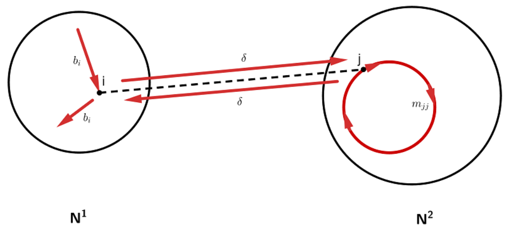
(Type IV) New walks starting at a node in and ending at a node in . This part is similar to Type III and contributes to equation (39).
Appendix C Interventions in alternative network models
Our paper is applicable to many other network models in which Katz-Bonacich centrality plays an important role in shaping the equilibrium. We list several models. A common theme is that Katz-Bonacich centrality, similar to Ballester et al. 2006, is a building block of the equilibrium objective.
- 1.
(Multiple activities) Chen et al. 2018b consider a network model with multiple interdependent activities. In the network , each player can choose the levels of two activities with utility
where is ’s characteristics; is the cost of action ; and captures the network externalities. Chen et al. 2018b show that if , there exists a unique Nash equilibrium given by
where . That is, the equilibrium profile is the weighted sum of two Katz-Bonacich centralities.
- 2.
(Direct complements and indirect substitutes)
Currarini et al. 2017 introduce a linear quadratic network game in which each agent faces peer effects from distance-one neighbors but also exhibits local congestion effects from distance-two neighbors. Specifically, the payoff of individual is given by
where the last term is new compared with Ballester et al. 2006 and captures the strategic substitution effect between players at distance-two in the network. Note that and is the -th element of matrix . Under some regularity assumptions on and , Currarini et al. 2017 show that the unique equilibrium equals
In fact, we can rewrite the above equilibrium succinctly as a linear combination of two Katz-Bonacich centralities:
(41) where and . Note that and satisfy . Equation (41) directly follows from the following mathematical identity:
That is, the equilibrium in Currarini et al. 2017 equals the weighted sum of two Katz-Bonacich centralities.
- 3.
(Local complementarity and global substitution) In addition to local complementaries, players might experience global competitive effects. In one extension, Ballester et al. 2006 consider the following utility function of individual :
where the term is the global interaction effect that corresponds to a substitutability in efforts across all players. measures the intensity of the global interdependence. For simplicty, we assume that each player’s intrinsic marginal utilities are identical. Ballester et al. 2006 show that the equilibrium behavior in this network game is
Each player’s equilibrium strategy is a function of Katz-Bonacich centralities. In particular, the aggregate equilibrium action, , is a monotonic function of .
Since the equilibrium in each of these models is either linear combinations or transformations of the Katz-Bonacich centralities, we can directly apply Proposition 1 to study the effects of structural and chracteristical interventions, and study similar issues such as the key group and the key link problems.