A note on synthesizing geodesic based contact curvesJournal: Mechanism and Machine Theory

Robotic grasping and manipulation is achieved through the interaction of robotic fingers with objects [1, 2, 3]. In order to carry out the manipulation, the robotic fingers either roll [4, 5, 6], slide [7, 8] or stick [9] on the object surface or use a combination of all three motions [10]. Rolling contacts during in-hand manipulation are known to accord a larger workspace to the object being manipulated by robotic fingers [11]. The relative motion of the object with respect to the fingertips generates contact curve on the object as well as on the fingertips [12]. The gross motion of the object is related to the contact curves if the type of relative motion (sliding, rolling, or a combination of sliding and rolling) is known [12].

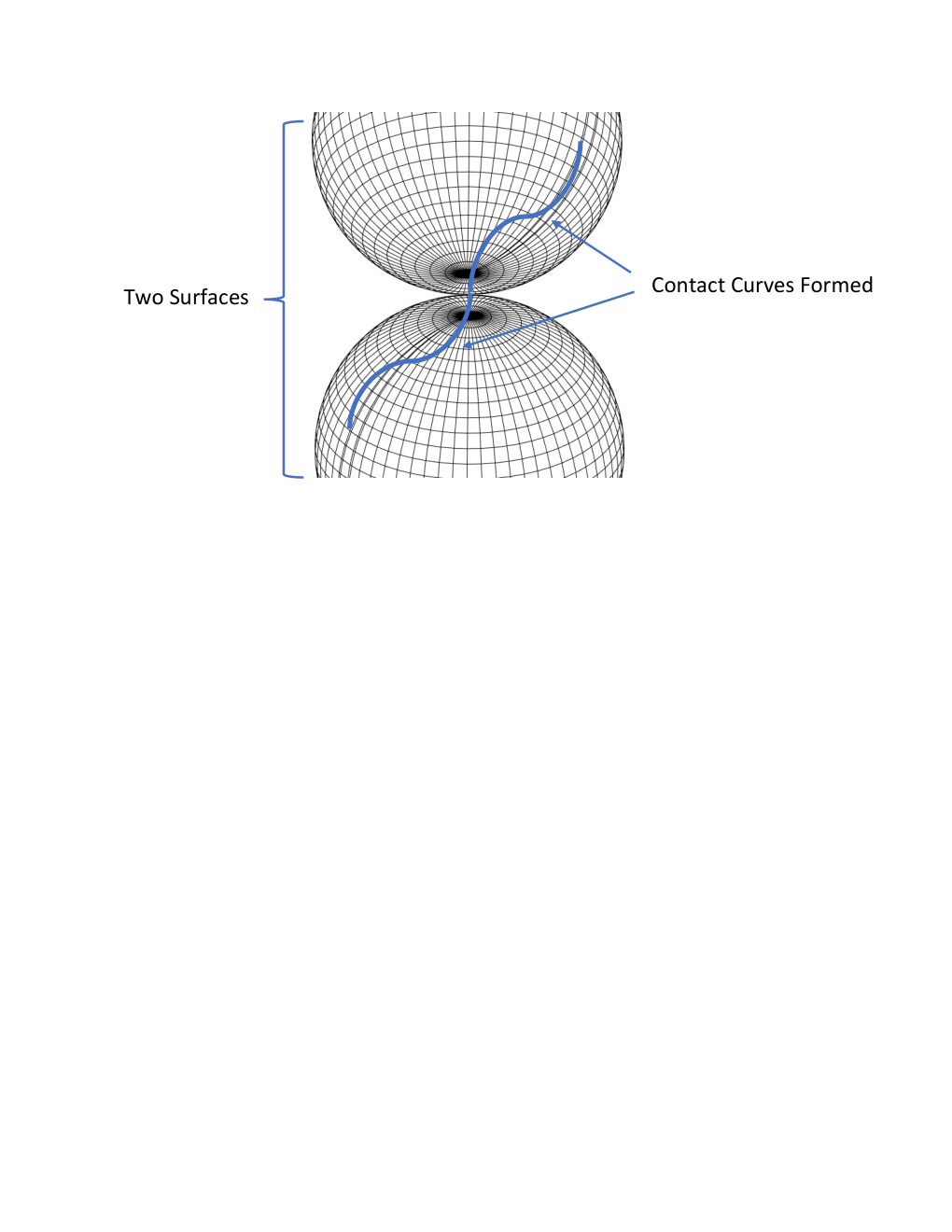
The contact curve is the locus of the instantaneous point of contact between two contacting surfaces in relative motion and is formed on both the surfaces (as shown in Figure 1). For planar two dimensional objects, the contact curves are restricted to lie along the contact edge only. However, for three-dimensional contacts, as encountered during in-hand manipulation of objects, spatial contact curves are formed. There have been an interest in analysing the contact curves generated for a specific type of relative motion. The differential constraint equations constraining the relative motion of objects leading to the generation of contact curves were formulated for both rolling and sliding during the late 1980s [12]. These algebraic equations relate the time derivative of the coordinates attached to the surfaces to the instantaneous linear and angular velocities of the two rigid bodies. Montana’s contact curve equations [12] have also been utilised to formulate control strategies to ensure that an enhanced grasp pose is achieved [13]. The grasp angle is defined as the angle between the contact force vector and surface normal at the point of contact. The control algorithm [13] was based on minimizing the grasp angle during in-hand manipulation. Although the generalised contact equations have not seen much implementation, the rolling contact equations have been utilised for simulation and control of robotic fingers [5] in contact with the object. Choudhary and Lynch [14] have also used these equations to synthesize single input control of a sphere in a bowl. The equations were also utilised to plan contact curves on the surface of the sphere [15]. Although Montana’s equations [12] have been widely used for simulation and control purposes, they relate only the first-order derivatives of the contact curves to the velocities of the object. Sankar et al. [16] associated the second-order derivatives of the surface variables (like the curvature form) with the acceleration of the body. This conjecture was useful to associate surface geometry with the dynamics of the system.

Contact curves have also been utilised to formulate exact forward and inverse kinematics during rolling motion [17], and to formulate a polynomial order computation of motion under rolling contact leading to reduction in computation time [18]. The contact acceleration equations derived in [16] have been used to formulate feedback linearizable control structures that admit control of the gross motion of the object as well as the differential motion of the fingers on the object [19]. The method was presented by Sarkar et al. [19], where the motion of the fingers was used to control the net object motion and the contact curve generated on the object surface.

Researchers have also focussed on analysing the nature of the contact curves formed for a particular type of relative motion. An adjoint-based approach was developed for a sliding - rolling system [20]. A Darboux-frame based approach has been formulated for rolling contact motion [21]. Contact curves have also been utilised to plan the initial motion of sliding/ rolling systems to avoid obstacles [22] while rolling.

Though the use of contact curves have been demonstrated, the contact curves have not been utilised to get a desired relative motion (like rolling). The methods stated above do not focus on generating contact curves to get the desired motion. However, there have been few instances where the contact curves were related to the type of motion. During the 1990s, a finger gaiting methodology formulated by Han et al. [23] concluded that rolling on great circles on a spherical object will lead to great circle contact curves on the spherical finger as well. This was one of the first instances where the generation of a particular type of contact curve was related to the rolling motion. Later, Lei et al. [24] utilised contact curves to show that if two bodies are in rolling constraint, then two geometrical invariant properties (torsion form and the curvature form) completely define the relative angular velocity. It was shown that the difference between the geodesic curvatures of the two contact curves formed on contacting bodies is zero during rolling.

A Geodesic curve is formally defined as the path with the shortest distance between two points on a surface [25], and have been studied intensely in the field of differential geometry. The same curve can also be defined as the trace of a particle moving on a surface with acceleration purely normal to the surface. In an extension to dimensions higher than $\mathbb{R}^{3}$, geodesic contact curves are defined in terms of the second-order Christoffel symbols [26] as per equation 1.

where $\psi_{t}$ represents the $t^{th}$ coordinate on the manifold (n-dime nsional) immersed in $\mathbb{R}^{m}$ for t = 1:n and $\Gamma^{i}_{jk}$ represents the Christoffel symbols of the second kind for the manifold. Any object surface in three dimensions can be considered as a 2-dimensional manifold immersed in $\mathbb{R}^{3}$. Hence, two geodesic equations are generated. For a real object surface (2-D), the symbol $\psi_{t}$ represents the surface coordinates (called chart variables). Points on the surface can be represented by a 2-D parametric function (chart function). It should be understood that the geodesic equations do not define exact coordinates of contact curves but relate the second-order derivative of the growth of surface coordinates (chart variables) to the growth of the first-order derivative of the coordinates at a given location. In this paper, we prove some results related to rolling motion, focussing on cases where geodesic curves are formed due to typical motion resulting from an object being manipulated by fingers. This includes proof of guaranteed no-slip motion if the finger and the object contacts move on geodesic curves at all times. Geodesics are not natural attractors and hence do not ensure proper disturbance rejection. A modification to the classical geodesic equation is proposed, which ensures proper disturbance rejection. The modification is done by driving the system (the system which generates the contact curves) to a contracting region [27].

In this paper, we show that if geodesic based contact curves are generated on the surface of contacting bodies, then rolling constraints are maintained. The classical differential geodesic equations in surface coordinates are modified to synthesize a relationship between the growth of geodesic curves and the relative velocity between the contact frames. A further modification to the classical geodesic equations is shown to reject sliding disturbances between the contact frames. The methodology provides a kinematic approach to ensure that the relative contact velocity reduces to zero after perturbation. Apart from the proof that geodesic based contact curves result in rolling constraints, a corollary to the proof is also presented. The corollary states that if the contacting bodies demonstrate rolling constraint and one of the contact curve is a geodesic, then the contact curve on the other contacting body will also be a geodesic curve. The derivations of the expressions of relative acceleration and relative velocity (using contact curves) are inspired by the methods in [16], but the expressions are reformulated to make them amenable to treatment using classical differential geometry. The methodology developed can be used to sustain rolling constraints during rolling in-hand manipulation of the object. The fingertips can map the geodesic based trajectories such that the resulting contact curves on the surface of the finger and the surface of the object are geodesics.

Although the method is developed considering inhand manipulation of an object, the method can be used to maintain rolling constraints for any set of contacting bodies and the proofs provided in the paper are applicable to general contacting rigid bodies. The hard fingertip can be replaced by any actuated body (or manipulator) and the interacting object can be fixed or free to be manipulated. A manipulator rolling its end effector over a manifold is one such instance. The contributions of the paper can be summarized as:

• 1.

  Understanding the nature of contact between bodies in relative motion when the trace of the contact points on the body surface are geodesics and its correlation to rolling contact. A proof relating the existence of rolling contact between the contacting frames and the synthesis of geodesic based contact curves is presented. The architecture is studied in context of in-hand manipulation of an object.

• 2.

  It is shown that when the progress of the contact is guided by a proposed modification to the geodesic based contact equations, it results in rejection of slip disturbances for two bodies in contact. The method can be used for synthesis of practical in-hand manipulation where rolling contact is desired. If the contacting bodies follow the modified geodesic equations, then rolling contact can be regained post slip.

• 3.

  A proof to a corollary is presented. The corollary states that if geodesic contact curves are known to be maintained on one contacting body, then geodesic based contact curves will be synthesised on the other contacting body as well, if rolling constraints are satisfied at all times.

Consider two rigid bodies in contact. For each rigid body, three associated frames are identified, as shown in Figure 2. The frame $G_{i}$ is attached, preferably to the geometric center of the body. The frame $C_{i}$ is attached to the body and is located at the contact point on the surface of the rigid body in consideration. Let there be another frame ($E_{i}$), moving on the surface of the body, instantaneously coincident with the point of contact. The distance between the frames $C_{i}$ and $E_{i}$ is instantaneously equal to zero (by definition), but the relative velocity between the two frames may be non-zero. With the evolution of time, $E_{i}$ follows the instantaneous contact points (origin of instantaneous $C_{i}$ frame) synthesized on the surface of the body, describing a locus, which is the contact curve. The three frames ($C_{i},G_{i}~\text{and}~E_{i}$) can be assigned for each body in contact. The relative slip between the two bodies in contact is tracked by the instantaneous relative velocity between the $C_{i}$ frames attached to each body.

In order to formulate the contact kinematics in terms of surface properties, the local surface coordinates are mapped to a cartesian system using localised chart functions. The chart maps the surface coordinates of points on a surface to its cartesian coordinates. Let the position vector of the contact point ($\mathbf{r}$) be represented in terms of the local surface coordinates (u(s),v(s)) using the standard chart function f(u,v). The coordinate frame attached to $E_{i}$ is a natural coordinate frame defined by: $[\frac{\frac{\partial\textbf{f}}{\partial u}}{||\frac{\partial\textbf{f}}{\partial u}||},\frac{\frac{\partial\textbf{f}}{\partial v}}{||\frac{\partial\textbf{f}}{\partial v}||},\frac{\frac{\partial\textbf{f}}{\partial u}\times\frac{\partial\textbf{f}}{\partial v}}{||(\frac{\partial\textbf{f}}{\partial u}\times\frac{\partial\textbf{f}}{\partial v})||}]$. The velocity of the frame $E_{i}$ with respect to frame $G_{i}$ and written in the $G_{i}$ frame is given by equation 2.

The rotation matrix relating the rotation of the $E_{i}$ frame is given by equation 3.

where $\hat{\mathbf{n}}=\frac{\frac{\partial\mathbf{f}}{\partial u}\times\frac{\partial\mathbf{f}}{\partial v}}{||\frac{\partial\mathbf{f}}{\partial u}\times\frac{\partial\mathbf{f}}{\partial v}||}$, $\mathbf{n}={\frac{\partial{\mathbf{f}}}{\partial u}\times\frac{\partial{\mathbf{f}}}{\partial v}}$. So, the angular velocity of the frame $E_{i}$ represented in frame $G_{i}$ is given by:

where $\mathbf{R_{i}}=\left[{\frac{\partial\textbf{f}}{\partial u}},{\frac{\partial\textbf{f}}{\partial v}},{\frac{\partial\textbf{f}}{\partial u}}\times\frac{\partial\textbf{f}}{\partial v}\right]$ and $\mathbf{K_{i}}^{-1}=\left[\begin{array}[]{ccc}||\frac{\partial\textbf{f}}{\partial u}||&\textbf{0}&\textbf{0}\\ \textbf{0}&||\frac{\partial\textbf{f}}{\partial v}||&\textbf{0}\\ \textbf{0}&\textbf{0}&||\textbf{n}||\end{array}\right]$

The acceleration of the frame $E_{i}$ with respect to the frame $G_{i}$ is given by equation 7.

The angular acceleration of the frame $E_{i}$ is given by equation 8.

Let $\frac{\partial\mathbf{\hat{f}}}{\partial u}={\upzeta_{1}}$ and $\frac{\partial\mathbf{\hat{f}}}{\partial v}=\upzeta_{2}$, then the terms in equation 8 take the form:

We have thus derived the measures needed to write the kinematics equations, in cartesian frames. The kinematic equations are written here in terms of the surface coordinates and their time derivatives.

Consider a case of in-hand manipulation of the object using hard fingers (Figure 4). By hard fingers (or rigid body), we mean that the finger has a representative point of contact. The process of manipulation with the contacting body (or fingertip) is desired to be a pure rolling motion. We assume that the contacting body (or the fingertip) does not spin about the local normal of the object at contact.

For robotics grasping, it is required that the fingers combine to apply forces to ensure that the contact between the object and the fingertip is always maintained. In this paper, we do not specifically look at means of ensuring contact and start by examining the interaction of the contact of the object with one of the fingers in isolation while the object is being manipulated. The interaction of the fingertip with the object can be generalized to any active rigid body (or manipulator end effector) interacting an object without break of contact. Throughout the derivation, the manipulating rigid body (fingertip) is referred to as body 1 whereas the the object is referred to as body 2. To derive the expressions of relative acceleration and relative velocity using contact curves, the methods presented by Sankar et al. [16] are useful.

The frames associated with body 1 and the object manipulated (body 2) is as shown in Figure 3. In this formulation, the vector joining origin of frames (say $A$ to say $B$) is represented as $\mathbf{r}_{AB}$. The velocity of a frame (let $B$) with respect to the frame (let $A$), as observed in frame (let $K$), is represented as ${}^{K}\mathbf{v}_{AB}$. Similarly, the acceleration of a frame (let $B$) with respect to the frame (let $A$), observed in frame (let $K$) is written as ${}^{K}\mathbf{a}_{AB}$ and, the angular velocity of frame (let $A$) as observed in frame (let $K$ ) is written as ${}^{K}\mathbf{\omega}_{A}$.

In order to relate the acceleration of the frames attached to respective bodies ($C_{1}$ and $C_{2}$), consider a triangle of infinitesimal sides at the contact point (connecting points $E_{1}~\text{to}~C_{2}~\text{to}~C_{1}~\text{to}~E_{1}$) (Figure 5 (a)). For these two contacting bodies, using triangle law of vector addition, we get:

Writing all the terms in equation 10 in the frame $C_{2}$, and differentiating equation 10 with respect to time in reference frame $C_{2}$ results in:

We note here that $\mathbf{r_{C_{1}E_{1}}}$ is conveniently defined in frame $C_{1}$. Its derivative in frame $C_{2}$ consists of derivative of $\mathbf{r_{C_{1}E_{1}}}$ in frame $C_{1}$ and a term which is cross product of the relative angular velocity of the two frames with $\mathbf{r}_{C_{1}E_{1}}$. Differentiating once more in frame $C_{2}$, we relate the accelerations as:

We also know that $\mathbf{r}_{C_{1}E_{1}}$ is equal to zero as the two frames are coincident by definition. However, a non-zero relative velocity between the frame $E_{i}$ and the frame $C_{i}$ is allowed. So, equation 11 and equation 12 reduce to:

All the terms in equation 13 are written in frame $C_{2}$. Similarly, for another case of triangle addition (Figure 5 (b)), we get:

Again, differentiating the equation 14 twice with all the frames represented in $C_{2}$ yields:

As the contact frames $E_{1}$ and $E_{2}$ are by definition instantaneously coincident, so the relative velocity ${}^{E_{2}}\mathbf{v}_{E_{1}E_{2}}=0~\text{and}~\mathbf{r}_{E_{1}E_{2}}=0$ instantaneously. So, the equation 15 simplify into:

Similarly, differentiating equation 15 and substituting $\mathbf{v}_{E_{1}E_{2}}=0,\mathbf{r}_{E_{1}E_{2}}=0,{{}^{E_{2}}\mathbf{\dot{v}}_{E_{1}E_{2}}}=0$,$\mathbf{\dot{r}}_{E_{1}E_{2}}=0$ we get equation 17.

Substituting LHS of equation 16 and equation 17 in equation 13, we get equation 18.

Through out the paper, all the terms are observed in the $C_{2}$ frame only (irrespective of the frame of representation). The angular velocity of the body 1 (frame $C_{1}$) as observed in frame $C_{2}$ is given by: $\mathbf{\omega}_{rel}={}^{C_{2}}\mathbf{\omega}_{C_{1}}$. The relative angular velocity $\mathbf{\omega}_{rel}$ is then written in the $E_{2}$ frame as: $\mathbf{\omega}_{rel}=\left[\omega_{x}~\omega_{y}~\omega_{z}\right]^{T}$, with $\omega_{z}$ directed along the local contact normal and $\omega_{x}$ and $\omega_{y}$ directed along orthogonal local tangents. With the stipulation that the objects in relative contact are not allowed to spin about the contact normal, the angular velocity term $\mathbf{\omega}_{rel}~\text{reduces to}~\left[~\omega_{x}~\omega_{y}~0~\right]^{T}$. From yet another case of triangle law of vector addition (Figure 5 (c)), we have:

Differentiating equation 19 in $G_{i}$ frame results to:

As, the frames $C_{i}$ and $G_{i}$ are on the same rigid body, so ${}^{G_{i}}\mathbf{v}_{G_{i}E_{i}}={}^{C_{i}}\mathbf{v}_{C_{i}E_{i}}(\mathbf{r}_{C_{i}E_{i}}=0,{}^{G_{i}}\mathbf{v}_{G_{i}C_{i}}=0)$. By a similar argument, ${}^{G_{i}}\mathbf{a}_{G_{i}E_{i}}={}^{C_{i}}\mathbf{a}_{C_{i}E_{i}}$. Hence, the acceleration and velocity of the frame $E_{i}$ with respect to $G_{i}$ as observed in $G_{i}$ are equal to the acceleration and velocity of the frame $E_{i}$ with respect to $C_{i}$, as observed in $C_{i}$. We can state this equation form as:

In order to formulate the relative velocity or acceleration, it is important to write all the terms in the same frame (irrespective to the frame of observation). All the terms are written in the $E_{2}$ frame. Appropriate rotation matrices are used to change the frame of representation of vectors. Following this method, the relative acceleration between the frames $C_{1}$ and $C_{2}$ (equation 18), written in a frame attached to $E_{2}$ are obtained by premultiplying the rotation matrices.

where $\mathbf{R}_{1}$ and $\mathbf{R}_{2}$ represents the rotation matrices required to transform the acceleration terms from $G_{i}$ frames to one of the contact frames (here $E_{2}$). For this case, the rotation matrices $\mathbf{R}_{1}$ and $\mathbf{R}_{2}$ are:

where $\mathbf{R}_{\psi}=\mathbf{R}_{\psi}^{T}=\left[\begin{array}[]{ccc}cos\psi&-sin\psi&0\\ -sin\psi&-cos\psi&0\\ 0&0&-1\end{array}\right]$, and $\psi$ is the angle made by the $\frac{\mathbf{\partial f_{i}}}{\partial u_{i}}$ vectors corresponding to each contact curve on the two surfaces. The details of the syntesis of the rotation matrix ($\mathbf{R}_{\psi}$ for two contacting bodies is explained in detail in the literature [12, 13]). The matrix $\mathbf{R}_{\psi}$ is used to relate vectors written in $E_{1}$ frame to $E_{2}$ frame. The angle $\psi$ refers to the angle between the x-axis (u-curves) for the two contacting bodies.

Substituting $\frac{\partial\hat{\mathbf{f_{i}}}^{T}}{\partial u_{i}}\frac{\partial{\hat{\mathbf{f_{i}}}}}{\partial u_{i}}=1$,$\frac{\partial\mathbf{\hat{f_{i}}}^{T}}{\partial v_{i}}\frac{\partial\mathbf{\hat{f_{i}}}}{\partial v_{i}}=1$ and $\frac{\partial\hat{\mathbf{f_{i}}}^{T}}{\partial u_{i}}\frac{\partial\hat{\mathbf{f_{i}}}}{\partial v_{i}}=0$ and by using the definitions of second order Christoffel symbols (equation 24), we simplify the expression of relative acceleration terms. The elements $\frac{\partial\hat{\mathbf{f_{i}}}^{T}}{\partial u_{i}}\frac{\partial\hat{\mathbf{f_{i}}}}{\partial v_{i}}$ are the non diagonal terms of the metric tensor [28] of the surface. It is known that the natural coordinate system (u,v) is orthogonal. So by definition, the non diagonal elements of the metric tensor are equal to zero, that is, $\frac{\partial\mathbf{f_{i}}}{\partial u_{i}}^{T}\frac{\partial\mathbf{f_{i}}}{\partial v_{i}}=0$. So, the terms corresponding to the non diagonal elements of the metric tensor drop out of the formulation. Using the more compact resulting Christoffel symbols:

The equation for relative acceleration in equation 22 is rewritten as equation 25.

where $\mathbf{M_{i}}$ is given by $\mathbf{M_{i}}=\left[\begin{array}[]{ccc}||\frac{\partial\mathbf{f_{i}}}{\partial u_{i}}||&0&0\\ 0&||\frac{\partial\mathbf{f_{i}}}{\partial v_{i}}||&0\\ 0&0&1\end{array}\right]$. The first two rows represent the tangential direction and the last element represents the acceleration along the normal direction. In order to ensure brevity, the normal acceleration component is not derived explicitly and labelled as ‘*’. Similarly, the relative velocity can be written as equation 26.

Components of the relative velocity can be obtained by substituting the expression of rotation matrices and expression of $\mathbf{v}_{ei}$ as in equation 2 in equation 26.

The first two rows represent the velocities in the tangent plane to the surface at the contact point to the object. In order to restrict slipping, we need to ensure that the first two terms in the two rows in equation 25 are zero.

In order to plan the trajectory, it is useful to have a single variable parameterisation of the path parameters ($u_{i}(s),v_{i}(s)$) with respect to time. The rate of growth of the path parameter ‘s’ is related to time as $\sigma=\frac{ds}{dt}$. For a particular manipulation, the term $\sigma$ can be planned to be a time-varying polynomial. The rate of growth of path parameters $(u_{i}(s),v_{i}(s))$ with respect to time is represented by equation 28.

On differentiating equation 28, we get:

The expressions in equation 29 are reformulated to obtain second order path derivatives:

The equation 28 and equation 30 relate the first and second time derivative of the growth of surface coordinates to the first and second derivatives with respect to the path parameter ‘s’. This reformulation allows computation of geodesics in terms of time derivative of the surface coordinates. The geodesic curve is commonly expressed in differential form [26] in terms of the path parameter ‘s’:

The equation 31 is written in terms of the derivatives of the surface coordinates with respect to the path parameters. To obtain the geodesic equations in terms of the derivatives of the contact coordinates with respect to time, the terms relating $\frac{du_{i}}{ds},\frac{dv_{i}}{ds},\frac{d^{2}u_{i}}{ds^{2}},\frac{d^{2}v_{i}}{ds^{2}}$ (in equation 28 and 30) are substituted in equation 31. The time dependent version of equation 31 results in equation 32.

We shall call the reformulated governing equation 32 as a time parameterized geodesic trajectory. Substitute expressions of $\ddot{u}$ and $\ddot{v}$ (from equation 32) in equation 22, to get an expression of $a_{rel}$ as in equation 33.

where $n_{1}$, $n_{2}$, $n_{3}$ and $n_{4}$ are defined by:

and, equivalently equation 35.

We see that the expression $\mathbf{a}_{rel}$ is a scalar multiple of the expression of $\mathbf{v}_{rel}$ in equation 27 and can be conveniently written as:

The equation 36 suggests that the time parameterized geodesic based trajectory of the contact point on the two contacting bodies leads to a relative acceleration which is a scalar multiple of the relative tangential velocity between the object and the finger. For the case of the relative velocity being zero at the start of the manipulation, the relative acceleration between the contacts will be zero for all subsequent time instances. Also, in case the rate of change of the position of the contact point with path parameter on the object being identical to or a constant scalar multiple of the time rate of change of the contact point ($\sigma=\text{constant},\dot{\sigma}=0$), then a reformulation of equation 34, results in $n_{i}=0$ for i = 1:4. This suggests that the relative acceleration of the origin of the two contacting frames is equal to zero. If $\sigma=\text{constant}$, then the equation 36 simplifies to:

To interpret equation 37, consider a second order rolling condition, which is satisfied between two bodies in contact and relative motion if both the relative velocity and the relative acceleration of the instantaneous contact point is zero. If no slip is ensured for finite time $\delta t$, that is, if $v_{rel}$ = 0 over a time interval $\delta t$, then the relative tangential acceleration is zero at all times, ensuring second order rolling between the finger and the object. As a particular case, if $\sigma$ is planned to be a zero-order polynomial (constant value), that is, $\dot{\sigma}=0$, then the contact should necessarily be initiated contact with an initial relative velocity. In case the initial relative velocity at contact is zero, the contacting bodies will not move each other. So, this is not an attractive option. Hence, a proper design requires $\sigma$ to be time-varying entity, perhaps a higher-order polynomial.

In order to prevent slip during manipulation, the locus of the contact point should map geodesic curves on the fingertip (body 1), and conversely, the contact curve on the object should be geodesic as well. We note that the proof has been derived for exact geodesic trajectories. Though conceptually simple, the method is limited as it requires that the relative velocity between the contacting bodies to be maintained at zero for a small but finite time $\delta t$. This method also requires that the contact trajectory strictly follows the based contact curve at all time instances. We hence have no means of proper disturbance rejection if the contact trajectory deviates from the geodesic. It is understood that a practical system will be realisable if the contact curves are natural attractors, thus enabling proper disturbance rejection. In order to ensure proper disturbance rejection, the underlying geodesic trajectories are modified (section 4).

In order to ensure proper disturbance rejection for the trajectories, that is, in the case the contact system acquires relative velocity (sliding), then the trajectory should be controlled such that the relative velocity tends to zero asymptotically. This can be done by modifying the relationship (equation 36) between $\mathbf{a}_{rel}$ and $\mathbf{v}_{rel}$ in equation 36 to the form in equation 38.

where $\eta$ is a positive scalar. A selection of $\eta$ ensures that the system is in a contraction region [27] with $\frac{\dot{\sigma}}{\sigma}-\eta\sigma^{2}$ being negative over the entire trajectory. Correspondingly, the governing equations for contact curves are modified from equation 32 to equation 39. The trajectory on body 1 (fingertip) remains the same as earlier. Only the equations governing the geodesic curve mapped on the object (body 2) change as a result of this modification.

Contacts satisfying equation 39, ensure disturbance rejection if the fingertips (body 1) instantaneously slip on the object (body 2) or a lateral disturbance is forced by the environment. The modified geodesic equations can be used to define the contact curve at the next instance $\left\{(u_{1},v_{1}),(\dot{u}_{1},\dot{v}_{1}),(u_{2},v_{2}),(\dot{u}_{2},\dot{v}_{2})\right\}$ when the contact is known during relative slip. The right hand side terms of the third and the fourth equation grow to non zero values when the contacting frames show relative slip. The modified growth of contact curves on the surface of the object (or body 2) lead to rejection of slip. The modified geodesic trajectories converge to being exact geodesic trajectories once the relative velocity goes to zero.

References

- Andrychowicz et al. [2018] M. Andrychowicz, B. Baker, M. Chociej, R. Jozefowicz, B. McGrew, J. Pachocki, A. Petron, M. Plappert, G. Powell, A. Ray, et al., Learning dexterous in-hand manipulation, arXiv preprint arXiv:1808.00177 (2018).
- Sundaralingam and Hermans [2018] B. Sundaralingam, T. Hermans, Geometric in-hand regrasp planning: Alternating optimization of finger gaits and in-grasp manipulation, in: 2018 IEEE International Conference on Robotics and Automation (ICRA), IEEE, pp. 231–238.
- Chong et al. [1993] N. Y. Chong, D. Choi, I. H. Suh, A generalized motion/force planning strategy for multifingered hands using both rolling and sliding contacts, in: Proceedings of 1993 IEEE/RSJ International Conference on Intelligent Robots and Systems (IROS’93), volume 1, IEEE, pp. 113–120.
- Paljug et al. [1994] E. Paljug, X. Yun, V. Kumar, Control of rolling contacts in multi-arm manipulation, IEEE Transactions on Robotics and Automation 10 (1994) 441–452.
- Bicchi and Sorrentino [1995] A. Bicchi, R. Sorrentino, Dexterous manipulation through rolling, in: Proceedings of 1995 IEEE International Conference on Robotics and Automation, volume 1, IEEE, pp. 452–457.
- Maekawa et al. [1995] H. Maekawa, K. Tanie, K. Komoriya, Tactile sensor based manipulation of an unknown object by a multifingered hand with rolling contact, in: Proceedings of 1995 IEEE International Conference on Robotics and Automation, volume 1, IEEE, pp. 743–750.
- Shi et al. [2017] J. Shi, J. Z. Woodruff, P. B. Umbanhowar, K. M. Lynch, Dynamic in-hand sliding manipulation, IEEE Transactions on Robotics 33 (2017) 778–795.
- Spiers et al. [2018] A. J. Spiers, B. Calli, A. M. Dollar, Variable-friction finger surfaces to enable within-hand manipulation via gripping and sliding, IEEE Robotics and Automation Letters 3 (2018) 4116–4123.
- Chavan-Dafle and Rodriguez [2018] N. Chavan-Dafle, A. Rodriguez, Stable prehensile pushing: In-hand manipulation with alternating sticking contacts, in: 2018 IEEE International Conference on Robotics and Automation (ICRA), IEEE, pp. 254–261.
- Cherif and Gupta [1999] M. Cherif, K. K. Gupta, Planning quasi-static fingertip manipulations for reconfiguring objects, IEEE Transactions on Robotics and Automation 15 (1999) 837–848.
- WEILI and Kumar [1994] C. WEILI, V. Kumar, Workspace of planar cooperating robots with rolling contacts, Advanced robotics 9 (1994) 483–504.
- Montana [1988] D. J. Montana, The kinematics of contact and grasp, The International Journal of Robotics Research 7 (1988) 17–32.
- Han et al. [1997] L. Han, Y.-S. Guan, Z. Li, Q. Shi, J. C. Trinkle, Dextrous manipulation with rolling contacts, in: Proceedings of International Conference on Robotics and Automation, volume 2, IEEE, pp. 992–997.
- Choudhury and Lynch [2002] P. Choudhury, K. M. Lynch, Rolling manipulation with a single control, The International Journal of Robotics Research 21 (2002) 475–487.
- Svinin and Hosoe [2008] M. Svinin, S. Hosoe, Motion planning algorithms for a rolling sphere with limited contact area, IEEE Transactions on Robotics 24 (2008) 612–625.
- Sankar et al. [1996] N. Sankar, V. Kumar, X. Yun, Velocity and acceleration analysis of contact between three-dimensional rigid bodies, Journal of applied mechanics 63 (1996) 974–984.
- Cui et al. [2017] L. Cui, J. Sun, J. S. Dai, In-hand forward and inverse kinematics with rolling contact, Robotica 35 (2017) 2381–2399.
- Cui and Dai [2015] L. Cui, J. S. Dai, A polynomial formulation of inverse kinematics of rolling contact, Journal of Mechanisms and Robotics 7 (2015) 041003.
- Sarkar et al. [1997] N. Sarkar, X. Yun, V. Kumar, Dynamic control of 3-d rolling contacts in two-arm manipulation, IEEE Transactions on Robotics and Automation 13 (1997) 364–376.
- Cui and Dai [2015] L. Cui, J. S. Dai, From sliding–rolling loci to instantaneous kinematics: An adjoint approach, Mechanism and Machine Theory 85 (2015) 161–171.
- Cui and Dai [2010] L. Cui, J. S. Dai, A darboux-frame-based formulation of spin-rolling motion of rigid objects with point contact, IEEE Transactions on Robotics 26 (2010) 383–388.
- Jia [2016] Y.-B. Jia, Planning the initial motion of a free sliding/rolling ball, IEEE Transactions on Robotics 32 (2016) 566–582.
- Han and Trinkle [1998] L. Han, J. C. Trinkle, Dextrous manipulation by rolling and finger gaiting, in: Proceedings. 1998 IEEE International Conference on Robotics and Automation (Cat. No. 98CH36146), volume 1, IEEE, pp. 730–735.
- Cui and Dai [2009] L. Cui, J. S. Dai, A coordinate-free approach to instantaneous kinematics of two rigid objects with rolling contact and its implications for trajectory planning, in: 2009 IEEE International Conference on Robotics and Automation, IEEE, pp. 612–617.
- Kumar et al. [2003] G. R. Kumar, P. Srinivasan, V. D. Holla, K. Shastry, B. Prakash, Geodesic curve computations on surfaces, Computer Aided Geometric Design 20 (2003) 119–133.
- Haw and Munchmeyer [1983] R. Haw, F. Munchmeyer, Geodesic curves on patched polynomial surfaces, in: Computer Graphics Forum, volume 2, Wiley Online Library, pp. 225–232.
- Lohmiller and Slotine [1998] W. Lohmiller, J.-J. E. Slotine, On contraction analysis for non-linear systems, Automatica 34 (1998) 683–696.
- Murray [2017] R. M. Murray, A mathematical introduction to robotic manipulation, CRC press, 2017.
- Miller [2017] S. Miller, Simscape multibody contact forces library, MATLAB Central File Exchange (2017).
- Zefran et al. [1998] M. Zefran, V. Kumar, C. B. Croke, On the generation of smooth three-dimensional rigid body motions, IEEE Transactions on Robotics and Automation 14 (1998) 576–589.