The MUSE Hubble Ultra Deep Field Survey XVI. The angular momentum of low-mass star-forming galaxies. A cautionary tale and insights from TNG50Thanks: This study is based on observations collected at the European Southern Observatory under ESO programmes 094.A-0289, 095.A-0010 and 096.A-0045.

The sAM $j\equiv J/M$ is, in general, given by

In practice, the two-dimensional version of the specific angular momentum, appropriate for an axi-symmetric disk, is used

where $R$ is the enclosed radius, $\Sigma(r)$ the surface brightness, and $v(r)$ the rotation velocity profile.

Regarding Eq. 2, the total angular momentum $j_{\rm tot}\equiv j(<\infty)$ is not observable directly as inherent surface brightness limitations preclude measurements beyond $R_{e}$ or at best 2$R_{e}$ (Marasco et al. 2019, e.g.,). For massive galaxies, probing $j$ up to $R_{e}$ or 2$R_{e}$, where the $j$ profile reaches its plateau, might be sufficient, but in low mass galaxies, that regime might be difficult to reach even in the local universe, as discussed in Posti et al. 2018a; Marasco et al. 2019. Thus, previous work often resorted to estimators for $j_{\rm tot}$ such as Eq. 3, which is discussed in § 2.2. Here, we use a 3D methodology (§ 2.3) that bypasses common approximations and similar in essence to the analysis of Mancera Piña et al. 2021 who used ^3DBarolo (Di Teodoro & Fraternali 2015). In § 3, we show with mock cubes from TNG50 that our 3D method combined with Eq. 2 does reproduce the true $j$ values, computed directly from Eq. 1.

It is worth noting that in order to determine $j_{\star}(r)$ from Eq. 2, one needs the stellar mass profile $\Sigma_{\star}(r)$ and the stellar rotation curve $v_{\star}(r)$. However, determining stellar kinematics beyond $z=0$ is challenging in SFGs (but see Guérou et al. 2017, for a first attempt) or even in passive galaxies with strong continuum (van de Sande et al. 2013; Bezanson et al. 2018; Cole et al. 2020, e.g.,). As a result, most studies of the $j_{\star}-M_{\star}$ relation use the star-forming gas $v_{{\rm H\alpha}}$ kinematics as a proxy for $v_{\star}$ (Burkert et al. 2016; Harrison et al. 2017; Swinbank et al. 2017, e.g.,). Two studies attempted to convert $v_{{\rm H\alpha}}$ to $v_{\star}$, Marasco et al. 2019 at $z=1$ and Posti et al. 2018a at $z=0$ using the asymmetric drift correction (Meurer et al. 1996; Dalcanton & Stilp 2010; Burkert et al. 2010).

Regarding the stellar mass profile $\Sigma_{\star}(r)$, it acts as the normalization factor in Eq. 2, and thus one only need to know the profile shape, namely the Sersic index and the half-light radius $R_{e}$. For SFGs, one can use the star-forming gas profile $\Sigma_{{\rm H\alpha}}$ (or $\Sigma_{\hbox{[{\rm O}{\sc\,ii}]}}$) as a proxy for $\Sigma_{\star}$ provided that the SF gas and stars have similar scale length ²² 2 This implicitly assumes a small or negligible bulge component., which is expected from the almost linear Kennicut-Schmidt relation (Kennicutt 1998; Genzel et al. 2010; Daddi et al. 2010; Bacchini et al. 2019). In fact, the ${\rm H\alpha}$ size $R_{\rm e,{\rm H\alpha}}$ to continuum size ratio $R_{\rm e,\star}$ has been found to be $\approx 1$ ³³ 3 This ratio is slightly mass-dependent beyond $10^{10}\hbox{$\rm\thinspace M_{\odot}$}$ reaching 1.2-1.3 at $10^{11}\hbox{$\rm\thinspace M_{\odot}$}$ in the KMOS3D survey (Wilman et al. 2020). from a very large sample of 3200 galaxies at $0.7<z<1.5$ with WFC3 imaging in Nelson et al. 2016, confirmed in our data as discussed in § 4.2.

In this paper, we measure the star formation rate (SFR)-weighted sAM $j_{\rm sfr}$ determined from the star-forming gas properties, namely $v_{\hbox{[{\rm O}{\sc\,ii}]}}(r)$ and $\Sigma_{\hbox{[{\rm O}{\sc\,ii}]}}(r)$, as a proxy for $j_{\star}$ following other studies (Burkert et al. 2016; Contini et al. 2016; Swinbank et al. 2017, e.g.,). This has the advantage that the measurement is self-contained (from ${\rm H\alpha}$ or [O ii]) and that a comparison to similar quantities from simulations can be performed. We use the notation $\tilde{j}_{\star}$ to designate $j_{\rm sfr}$ and in Section 3.4, we quantify the potential bias between $\tilde{j}_{\star}$ and $j_{\star}$ in the TNG50 galaxies.

Given the difficulties in measuring $j(<r)$ in the outskirts of galaxies, a method that is commonly used in the literature (Burkert et al. 2016; Swinbank et al. 2017; Harrison et al. 2017; Gillman et al. 2020, e.g.,) for estimating $j_{\rm tot}$ is the following formulae (Romanowsky & Fall 2012, hereafter RF12):

where $R_{\rm e}$ is the half-light radius, $v_{s}$ the rotation velocity at $2R_{e}$, $v(2\,R_{e})$, and $k_{n}=1.15+0.029\cdot n+0.062\cdot n^{2}$ is a constant that depends on the Sérsic 1963 index $n$. Eq. 3 reduces to the well-known $j_{\rm tot,RF}=2\,v_{s}\,R_{d}$ for disks with $R_{d}$ being the exponential scale length.

However, we caution the reader against using Eq. 3 for low mass galaxies with ${\rm\thinspace log}(M_{\star}/\hbox{$\rm\thinspace M_{\odot}$})<9.5$–10, for the following reasons. Eq. 3 assumes that the velocity profile $v(r)$ is a constant from $r=0$, which might be appropriate for galaxies with ${\rm\thinspace log}(M/M_{\star})>10$, but is less suitable for intermediate and low mass galaxies, which are known to have slowly rising rotation curves (Persic et al. 1996; Catinella et al. 2006, e.g.,). Consequently, Eq. 3 can lead to an over-estimation of the total angular momentum as discussed in Obreschkow & Glazebrook 2014.

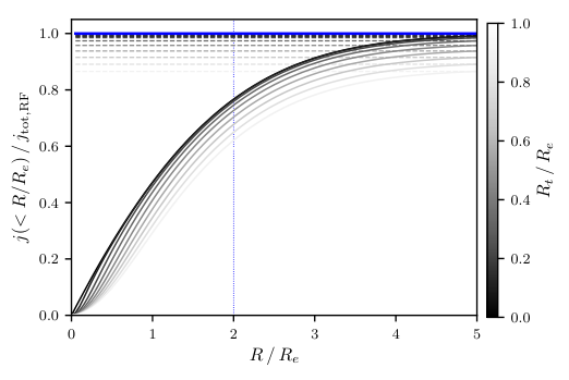
To quantify the overestimation in the low-mass regime, we show in Fig. 1(a) several sAM profiles (solid lines), corresponding to “tanh” rotation curves, $v(r)=V_{\rm max}\tanh(r/R_{\rm t})$ with varying inner slopes (parameterized by the turn-over radius $R_{\rm t}$), normalized to the RF12 approximation (represented by the blue horizontal line). This figure shows that, for galaxies with slowly rising rotation curves, that is with $R_{\rm t}/R_{e}$ of order unity, Eq. 3 results in an overestimation of the angular momentum by up to 15%. Obreschkow & Glazebrook 2014 made a similar point using rotation curves $v(r)\propto(1-\exp(-r/R_{\rm t}))$.

Moreover, there can be significant differences between the often used $k_{n}$ approximation, namely $k_{n}=1.15+0.029\cdot n+0.062\cdot n^{2}$ and the exact expression (derived in Appendix A) given by:

that can be as large as 15% for Sérsic indices $n\lesssim 1$ as indicated in Fig. 1(b).

In conclusion, combining these two effects, Eqs. 3 and 4, can lead to an overestimation of the sAM (up to 20–25%) for galaxies with $n\lesssim 1$ and/or when the rotation curve is slowly rising, that is in the low-mass regime at $M_{\star}<10^{9.5}\hbox{$\rm\thinspace M_{\odot}$}$. In addition, such galaxies with a large turn-over radius $R_{\rm t}$ tend to have large sizes and hence a low surface brightness, and thus their true $V_{\rm max}$ is more difficult to measure beyond $R_{\rm t}$.

In order to estimate $j$ directly from Eq. 2, one needs the intrinsic (deprojected and free from instrumental and resolution effects) velocity and surface brightness flux profile and these can be measured directly from 3D (position-position-velocity) data using the GalPaK^3D algorithm⁴⁴ 4 Available at http://galpak3d.univ-lyon1.fr. described in Bouché et al. 2015.

Briefly, GalPaK^3D performs a parametric fit on emission line data for the morphology and kinematics simultaneously directly onto the 3D data using a 3D ($x,y,\lambda$) disk model which specifies the morphology and kinematic profiles. For the morphology, the model assumes a Sérsic 1963 surface brightness profile $\Sigma(r)$, with Sérsic index $n$. For the kinematics, the model assumes a parametric form for the rotation curve $v(r)$ and for the dispersion $\sigma(r)$ profile. The model parameters are the centroid position $x$, $y$, $z$, the total line flux, the inclination $i$, the major-axis position angle P.A, the half-light radius ($R_{\rm e}$), the turnover radius $R_{\rm t}$ and maximum velocity $V_{\rm max}$ for the rotation curve, and the velocity dispersion $\sigma_{\rm 0}$, described below.

The rotation curve $v(r)$ can be ‘‘arctan’’, ‘tanh’ or other analytical forms as described in the documentation ⁵⁵ 5 See http://galpak3d.univ-lyon1.fr/doc/.. As described in Bouché et al. 2015, the velocity dispersion profile $\sigma(r)$ is made of three components added in quadrature. The first component $\sigma_{1}$ is that of a thick disk (Genzel et al. 2008), namely $\sigma_{1}(r)/v(r)=h_{z}/r$ where $h_{z}$ is the disk thickness, taken to be $0.2\times R_{\rm e}$. The second component $\sigma_{2}$ is comes from the natural broadning of the 3D disk model of finite thickness. The third component $\sigma_{3}$ is an adjustable constant term $\sigma_{0}$, as in Genzel et al. 2008; Förster Schreiber et al. 2006; Cresci et al. 2009; Wisnioski et al. 2015; Übler et al. 2019 and describes any additional turbulent component to the kinematic dispersions.

GalPaK^3D convolves the model with the Point Spread Function (PSF) and the instrumental Line Spread Function (LSF), which implies that the parameters are “intrinsic”, that is corrected for beam smearing and instrumental effects. Here, we use a Moffat PSF as characterized in Bacon et al. 2017, and we use Eq. (7) of Bacon et al. 2017 for the LSF.

GalPaK^3D uses a simple Metropolis-Hasting (MH) algorithm to optimize the parameters whose posterior distributions are given by the chain posteriors. As described in Bouché et al. 2015, the GalPaK^3D implementation of the MH uses a nonstandard Cauchy proposal distribution which shortens the burn-in phase considerably, but suffers, like most MH algorithms, from the need to manually tune the width of the proposal distribution.

Since its initial release, the following improvements and new features have been implemented in GalPaK^3D. First, in order to quantify the chain convergence for each parameter, GalPaK^3D performs the Geweke 1992’s convergence diagnostic test for each of the parameters, which is a $Z$-test of equality of means (of two parts of the chain) where auto-correlation in the samples is taken into account. Second, GalPaK^3D can now adapt the widths of the Cauchy proposal distribution automatically. Third, and most importantly, GalPaK^3D is now (since v1.20) compatible with the emcee code (Foreman-Mackey et al. 2013). emcee has the advantage that its multi-walkers remove the need to tune the proposal distribution, but it has the disadvantage to retain the Normal proposal distribution which is very slow and inefficient in reaching convergence because the Gaussian function does not have broad wings. For our purposes, we combine the self-tuning of our fast MH algorithm implemented in GalPaK^3D with the emcee sampler once convergence is reached as follows: we first run the self-tuning of our fast MH algorithm with Cauchy sampling, and then use the emcee sampler once convergence is reached.

Furthermore, as illustrated in Fig. 2, we use the following two-step process. We first determine the morphological parameters by fitting a 2D Sérsic model to the collapsed [O ii] cube (i.e. a two-dimensional flux map), keeping the inclination $i$ free. This yields estimates of the morphological parameters, namely inclination, size and Sérsic index ($i_{\rm 2d}$, $R_{e,\rm 2d}$, $n_{\rm 2d}$). Then, we fit a 3D model with the Sérsic $n$ fixed to 0.5, 1, 2 or 4 based on $n_{\rm 2d}$, and tophat priors on the half-light radius $R_{\rm e}$ and inclination $i$ from the results of the 2D analysis (Fig. 2). For the kinematics, we choose a $\tanh(r/r_{t})$ rotation curve $v(r)$ after finding that it gives more robust measurements of $V_{\rm max}$ than a $\arctan$ profile. Finally, from the morphological and kinematics information, namely $\Sigma(r)$ and $v(r)$ we can compute $j$ using Eq. 2. The total sAM is then calculated from the $j(<r)$ profile at 10 $R_{\rm e}$ ⁶⁶ 6 Others uses $j(<R_{\rm e})$ (Cortese et al. 2016) or even $j(<R_{\rm max})$ where $R_{\rm max}$ is the last radius where $\Sigma_{\star}(r)$ can be measured (Posti et al. 2018a; Marasco et al. 2019; Mancera Piña et al. 2021, e.g.,), which is prone to biases..

For the velocity dispersion, we evaluate the intrinsic (deconvolved) velocity dispersion profile $\sigma(r)$ at $2R_{\rm e}$, namely $\sigma_{\rm t}\equiv\sigma(2R_{\rm e})$. This is a more reliable estimator of the dispersion in the outer regions from our parametrization discussed earlier. Indeed, the fitted parameter, $\sigma_{0}$, can approach zero in some galaxies when the kinematic dispersions ($\sigma_{1,2}$) is sufficient to describe the data. In the remainder of the paper, we use $\sigma(2R_{\rm e})$ as the total velocity dispersion $\sigma_{\rm t}$ of SFGs.

In summary, our 3D method has several advantages and avoids the shortcomings mentioned in the previous section. In particular, it includes all of the information available by combining the many spaxels with very low signal-to-noise ratio (S/N), down to $\sim$0.1 in the outer regions, which are inaccessible with 2D velocity maps. Second, it avoids the assumptions of the Eq. 3 formula, namely of flat rotation curves, which can lead to biases in the low-mass regime. Third, it takes into account the effect of the PSF convolution. And fourth, it is self-consistent and does not rely on external data to break the $i-V_{\rm max}$ degeneracy. It does, however, assume that SFGs have regular velocity fields. Our modeling is similar to the DYSMAL code used in Bouché et al. 2007; Cresci et al. 2009; Davies et al. 2011; Genzel et al. 2017; Genzel et al. 2020, but GalPaK^3D adjusts the model parameters directly to the raw 3D cube while DYSMAL fits the 1D flux, velocity and dispersion maps generated from a 3D model.

We select 100 SFGs from TNG50 at each of the $z=0.5$ and $z=1.0$ snapshots with stellar masses in the range $10^{8.5}\hbox{$\rm\thinspace M_{\odot}$}<M_{\star}<10^{10.5}\hbox{$\rm\thinspace M_{\odot}$}$. We selected SFGs with specific SFR within $\pm 2\sigma$ from the median sSFR, excluding galaxies with sSFR$<10^{-11}{\rm\thinspace yr}^{-1}$ in order to mimic the observational selection on SFGs with [O ii] emission. From this sample, we randomly select the final sample to have a uniform distribution in ${\rm\thinspace log}M_{\star}$ and limited the sample to the range of sizes matching the UDF sample, namely from 1.5 to 6.5 kpc (see § 4). This resulted in a sample of 158 SFGS.

Fig. 3 shows the location of the sample of 158 SFGs in the size–mass and sSFR–mass scaling relations. In both panels, the gray points and contours represent the distributions for the $z=1$ TNG50 SFGs and the red symbols represent the 158 selected SFGs at $z=0.5$ and $z=1.0$. On the left panel, the gray band represents the size–mass relation from van der Wel et al. 2014 and on the right panel, the gray band represents the main-sequence for UDF SFGs (Boogaard et al. 2018). In the left (right) panel, the $z=0.5$ galaxies are rescaled to $z=1$ according to the size (SFR) evolution found by van der Wel et al. 2014 (Whitaker et al. 2014), respectively. This figure shows that we selected SFGs with properties representative to the full underlying population around the size and SFR scaling relations for SFGs.

Finally, Fig. 4 shows high-resolution images of three representative star-forming galaxies where the two left columns show the stellar light (dust-free color composite of the (SDSS)r-g-(Johnson)B bands) and the two right columns show the SFR in the gas phase, face-on and edge-on.

Each of the 158 simulated SFGs is processed in the following manner to generate several mock MUSE mini-cubes, for a total number of mock cubes of 790. First, a cube of two spatial dimensions with bounds $[-N_{r}/2\Delta_{r},N_{r}/2\Delta_{r}]$ and one velocity dimension with bounds $[-N_{v}/2\Delta_{v},N_{v}/2\Delta_{v}]$ is generated with $N_{r}=30$ pixels in each spatial dimension and $N_{v}=40$ pixels in the velocity dimension. For $z=1$ ($z=0.5$), we use voxels of size $\Delta_{r}=1.65{\rm\thinspace kpc}$ (1.25 kpc) and $\Delta_{v}=50\penalty\ {\rm\thinspace km\thinspace s}^{-1}$ ($65\penalty\ {\rm\thinspace km\thinspace s}^{-1}$), respectively, which corresponds to the MUSE instrument specifications of $0.2{\rm\thinspace arcsec}$ and 1.25Å at a rest-frame wavelength of $\lambda_{\rm rest}=$3728Å (Bacon et al. 2017). Second, the center of this cube is placed at the position of the most bound resolution element of the simulated galaxy, which generally is very close to the center of rotation, and at the velocity of the galaxy center-of-mass. Third, the cube is rotated such that the plane defined by the two spatial dimensions is perpendicular to the eigenvector of the moment of inertia tensor of the galaxy that has the smallest eigenvalue, such that the galaxy appears “face-on”.

For each galaxy, we apply further rotations to generate mock cubes for 5 inclinations ($i=15,30,45,60$ and $75^{\circ}$), each at a random azimuthal orientation $\phi$ ⁷⁷ 7 In addition, 9 galaxies were tested with 5 different azimuthal orientations for each inclination.. The SFR in each voxel of the cube is then calculated by summing up the contributions from all simulation gas cells using a Gaussian kernel representing the Point-Spread-Function (PSF) and Line-Spread-Function (LSF) appropriate for non-AO MUSE observations. In particular, for $z=1$ ($z=0.5$) the PSF has a Moffat profile with $\beta=2.5$ and a ${\rm FWHM_{r}}$ of $0.625$ arcsec ($0.675$ arcsec) (Bacon et al. 2017), and the LSF has a Gaussian profile with ${\rm FWHM_{v}}=2.55$Å (2.75Å), respectively. The PSF and LSF FWHMs correspond to $5.15{\rm\thinspace kpc}$ ($4.25{\rm\thinspace kpc}$) and to $100{\rm\thinspace km\thinspace s}^{-1}$ ($143{\rm\thinspace km\thinspace s}^{-1}$), for $z=1$ ($z=0.5$), respectively.

Finally, we add noise to the mock MUSE cubes in order to match the range of S/N (spaxel^-1) of our MUSE observations, which have S/N_max of a few to $\sim$40 (see § 4). For galaxies with ${\rm\thinspace log}M_{\star}>9$ ($\leq 9$), we set the noise to 0.001 (0.0002) SFR yr^-1, respectively.

In TNG50, we measure the following quantities: the sAM, the maximum rotation velocity $V_{\rm max}$ and velocity dispersion $\sigma_{\rm t}$, as follows.

Specific angular-momentum. The SFR-weighted $\tilde{j}_{\star}(r)$ is calculated using Eq. 1 with $\rho(\mathbf{x})$ as the star-forming gas density, which corresponds to a [O ii] weighting, using the 3D positions, velocities and densities of all SF gas at a given radius. We then use the cumulative profile $\tilde{j}_{\star}(<r)$ to then define the total sAM from max$(\tilde{j}_{\star}(<r))$.

Velocity dispersion. The gas velocity dispersion $\sigma_{\rm t}$ is defined as the 1D line-of-sight dispersion assuming isotropy, namely it is equal to $\sigma_{3D}/\sqrt{3}$. Here, $\sigma_{\rm 3D}$ is the average (SFR-weighted) of the internal velocity dispersion of star-forming gas inside kpc-sized patches at galacto-centric radii of 1.5–2.5$R_{\rm e}$, a method similar to Pillepich et al. 2019. In order to account for thermal broadening for $T=10^{4}$ K gas, we incorporate a $\sigma_{\rm th}\approx 15.7\penalty\ {\rm\thinspace km\thinspace s}^{-1}$ component into $\sigma_{\rm 3D}$ by adding it in quadrature⁸⁸ 8 This approach follows in spirit the calculations in Appendix A of Pillepich et al. 2019. However, it is important to note that Pillepich et al. 2019, in method (ii) of their appendix, have inadvertently added $\sigma_{\rm th}\approx 15.7\penalty\ {\rm\thinspace km\thinspace s}^{-1}$ to their line-of-sight velocity dispersions, while for a $T=10^{4}$ K ideal monoatomic Hydrogen gas that value corresponds to the 3D velocity dispersion, as implemented in this work.. This definition of line-of-sight SFR-weighted velocity dispersion at $\sim 2R_{\rm e}$ has the advantage that it closely mimics our observations $\sigma_{\rm t}(2R_{\rm e})$ (see § 2.3).

Rotational velocity. The rotation velocity $V$ is calculated as the SFR-weighted mean of the azimuthal velocities of the same patches used for the calculation of the velocity dispersion.

We now apply the methodology described in § 2.3 to the sample of 790 mock cubes of 158 simulated galaxies in order to test the performances of GalPaK^3D in recovering the morphological (sizes, inclination) and kinematic parameters of realistic galaxies. We find that the inclination is recovered with a relative error of $\pm 12^{\circ}$ provided that $i\geq 30^{\circ}$, as found in Contini et al. 2016 (Bouché et al. 2015, see also). Consequently, we restrict the analysis to mock cubes with $i\geq 30^{\circ}$.

Fig. 5 shows the sAM profile $\tilde{j}_{\star}(<r)$ found when applying Eq. 2 and the 3D methodology described in § 2.3 on the massive galaxy shown at the top of Fig. 4. The 5 panels show the $\Sigma_{\rm sfr}$ map, the SB profile, the intrinsic velocity field, the intrinsic velocity profile, and the intrinsic $\tilde{j}_{\star}$ profile, respectively. The velocity and SB profile are computed on the pseudo-slit, represented by the two horizontal gray lines. The light gray solid lines represent the profiles recovered from our algorithm for each inclination ($i\geq 30^{\circ}$), each performed on 5 orientations in this case. The red solid lines in columns 2, 3 and 4 represent the $\Sigma_{\rm sfr}$, $v(r)$ and $\tilde{j}_{\star}$ profiles determined directly from the TNG50 data. In the right most panel, the blue horizontal tick marks show our estimates $\tilde{j}_{\star}({\rm 3D})$, while the red horizontal tick marks show $\tilde{j}_{\star}$ from RF12 (Eq. 3). Depending on the steepness of the $v(r)$ profile, the RF12 approximation can lead to an over-estimation of the total angular momentum by 15–25% for the reasons described in § 2. Fig. 5 suggests that our 3D method is able to recover the intrinsic $\tilde{j}_{\star}(<r)$ profile with less bias, even when the rotation curve deviates from our assumed parametrization $v(r)=\tanh$. Next, we investigate the difference between the estimated and true $\tilde{j}_{\star}$ as a function of S/N.

Figure 6(left) shows the measured total angular momentum, $\tilde{j}_{\star}$(3D), as a function of the true angular momentum (SFR-weighted) as measured directly from the simulation output (bottom subpanel), and their relative difference, ${\rm d}j/j\equiv(\tilde{j}_{\star}({\rm 3D})-j_{\rm true})/j_{\rm true}$ (top subpanel). The points are colored according to $M_{\star}$. The red circles represent the median of ${\rm d}j/j$ whose errorbars represent the $1\sigma$ standard deviation.

The histogram in the top panel of Fig. 6(left) shows the distribution of the relative errors ${\rm d}j/j$. This histogram shows that globally our method does recover the intrinsic angular momentum with no apparent bias. We can quantify this bias further as a function of galaxy mass in Fig. 6(right). Figure 6(right) shows, for 1-dex bins in ${\rm\thinspace log}M_{\star}$ (at 8.5, 9.5 and ${10.5}$), from top to bottom), the distributions of ${\rm d}j/j$ resulting from our 3D method (left column) or the RF12 method (right column). The red solid line represents the continuous density estimation of the distributions using a Gaussian kernel with bandwidth of 0.2. Quantitatively, the mean relative error ${\rm d}j/j$ for our 3D methodology is $<5$%, while for the intermediate and lower mass bins, the RF12 approximation (Eq. 3) can lead to a significant bias of $\approx 10$-15% for the reasons discussed in § 2. For the most massive galaxies with $M_{\star}>10^{10}\hbox{$\rm\thinspace M_{\odot}$}$, and with ${\rm\thinspace log}\tilde{j}_{\star}>3$, our method underestimates $\tilde{j}_{\star}$ compared to RF12, but it is important to note that our sample in the UDF (§ 4) has only a handful of SFGs in this regime.

The width of the distributions shown in Fig. 6 is consistent with the errors obtained with our methodology. Indeed, the width of the ratios of the errors to ${\rm d}j$ is consistent with a (Cauchy) distribution ⁹⁹ 9 The few outliers are producing a distribution with a heavier tail than a Normal distribution. of width unity. This implies that the errors obtained from our methodology are broadly representative of the true error ${\rm d}j$ on the measurement.

We return now to the top panel of Figure 6 where the relative difference ${\rm d}j/j$ is plotted as a function of the effective S/N, S/N_eff, following the discussion in Bouché et al. 2015. This effective S/N accounts for the fact that surface brightness (SB) alone is not sufficient to determine the accuracy in the fitted parameters, given that the compactness of the galaxy with respect to the PSF plays also an important role. As discussed in Refregier et al. 2012, in the presence of a PSF convolution, the relative errors on the major-axis $a$ scales as

where $A_{\rm o}$ is the observed central surface brightness in the central voxel, $R_{\rm PSF}$ is the radius of the PSF ($R_{\rm PSF}\equiv$ FWHM/2) and $R_{\rm e}$ the intrinsic half-light radius. After performing a Taylor expansion around $R_{\rm PSF}/R_{\rm e}\sim(1-x)$ with $x\equiv(R_{\rm e}-R_{\rm PSF})/R_{\rm e}$ and $|x|<<1$, one finds that Eq. 5 becomes in the regime where $R_{\rm PSF}/R_{\rm e}$ is $\simeq 1.0$ (Bouché et al. 2015, see):

The last step follows from the simple argument that a given exposure time sets the surface brightness limit per voxel, and hence the maximum S/N (in the central voxel or spaxel), S/N_max, is directly proportional to $A_{\rm o}$.

Considering the sAM is essentially determined by the product of $R_{\rm e}$ and $V_{\rm max}$, one can thus expect that the accuracy of $j$ follows Eq. 6, which is represented by the gray curve in the top panel of Fig. 6.

Finally, we end this section by quantifying the potential difference between the SFR-weighted $\tilde{j}_{\star}$ and the stellar mass-weighted $j_{\star}$ because in observations of high-redshift galaxies, as in § 4, one is often limited to the SFR-weighted $\tilde{j}_{\star}$. Using TNG50 $z=1$ SFGs in the parent sample, Figure 7 shows the relation between $\tilde{j}_{\star}$ and $j_{\star}$. While this figure shows that the relation becomes non linear in the low mass regime, with ${\rm\thinspace log}j_{\star}<1.5$, (as found by El-Badry et al. 2018, in the FIRE simulations), it also shows that, on average, ${\rm\thinspace log}\tilde{j}_{\star}$ is an estimate of ${\rm\thinspace log}j_{\star}+0.25$ dex over a wide range of sAM from 50 to 2000 ${\rm\thinspace km\thinspace s}^{-1}$ kpc, which is the relevant range for our study.

We exploit the 3’$\times$3’ observations taken with the MUSE instrument over the Hubble Ultra Deep Field (Bacon et al. 2017, HUDF;) to investigate the angular momentum of intermediate redshift galaxies using the methodology presented in § 2.3. The observations were performed on a mosaic of nine 1’$\times$1’ 10 hr pointings and contain a single 1’$\times$1’ 27hr pointing, but we concentrate on the mosaic sample to ensure a homogenous selection. In the MUSE UDF mosaic, there are 494 [O ii] emitters (Inami et al. 2017). These [O ii] emitters have stellar masses ranging from $10^{7.5}$ to $10^{11}$$\rm\thinspace M_{\odot}$, where the stellar masses are estimated (Boogaard et al. 2018, as in ) using the stellar population synthesis (SPS) code FAST (Kriek et al. 2009) assuming a Chabrier 2003 initial mass function with an exponentially declining star formation history. As discussed in the next section, most [O ii] emitters are rather faint, with only about $\sim$50% of the these having a S/N above $\sim 3$.

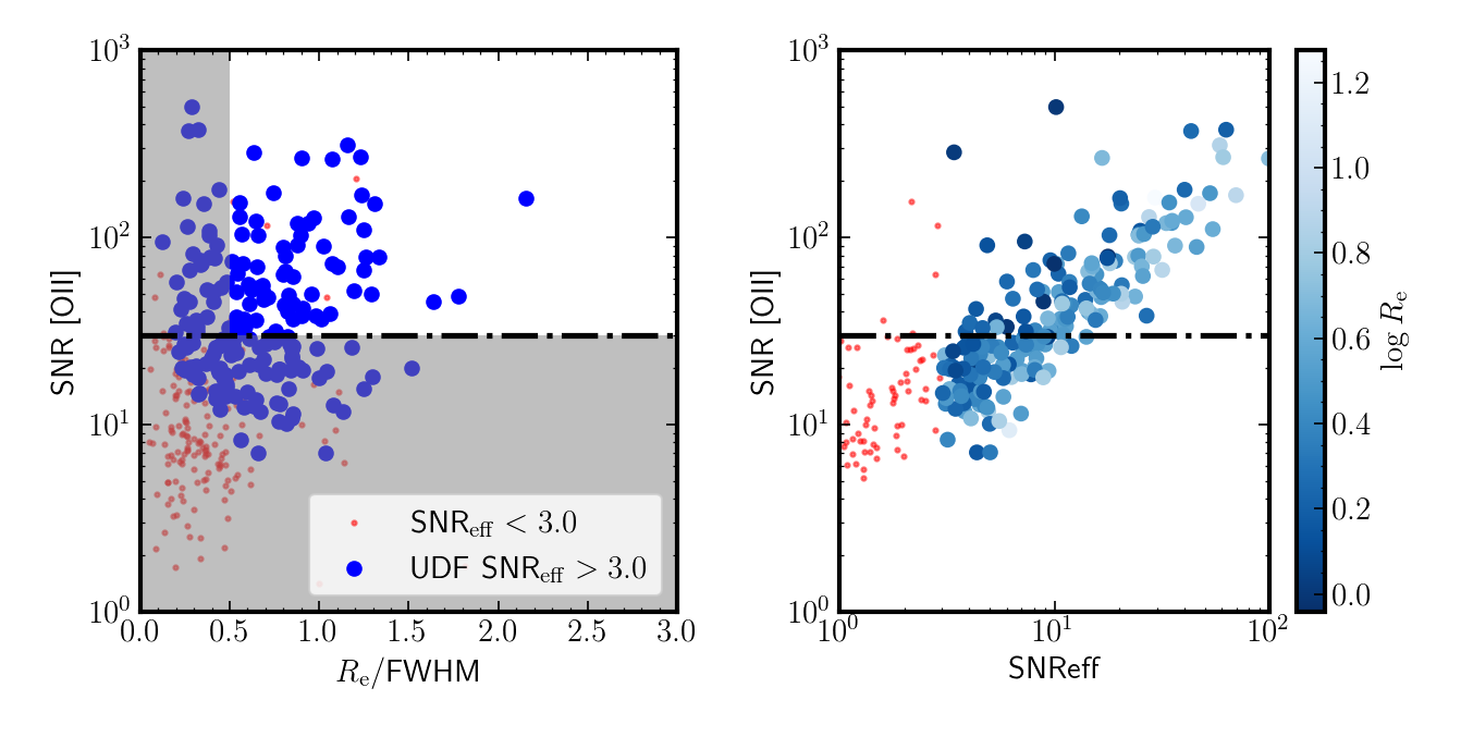
Figure 8 (left) shows the S/N of the total [O ii] flux as a function of the “resolved size” ($R_{\rm e}$ divided by the PSF FWHM) for the sample of SFGs, where the blue (red) points are SFGs with a S/N${}_{\rm eff}>3.0$ ($<3.0$), respectively. For comparison, the selection used in Abril-Melgarejo et al. 2021 is shown with the gray bands. The right panel compares the effective S/N and the total S/N, where the points are color-coded as a function of size $R_{\rm e}$, displaying the common surface-brightness biases. This figure shows that a S/N_eff 3, as determined in the previous section, opens the possibility to study the kinematics of faint galaxies, enlarging the sample by 30 to 50%.

Figure 9 shows the properties of the UDF sample in terms of sizes and SFRs as in Fig. 3. The sizes are the continuum-based $R_{\rm e}$ obtained from HST/F160W from van der Wel et al. 2014 and the SFRs are derived from SED fitting. The left panel shows the sample in the size-mass plane color coded as a function of the effective S/N, where the sizes were adjusted to $z=1$. For comparison, we show the size-mass scaling relation of van der Wel et al. 2014 and Mowla et al. 2019 down to $M_{\star}\sim 10^{8}\hbox{$\rm\thinspace M_{\odot}$}$. The TNG50 mocks used in § 3 are represented with the red small circles. The right panel shows the main-sequence or the SFR-mass plane where the points are color-code as a function of size. The points are scaled to $z=1$ where we used the main-sequence redshift evolution of Boogaard et al. 2018.

The first part of the methodology outlined in 2.3 is to determine the morphological parameters (size, inclination) by performing two dimensional Sérsic fits to the [O ii] flux maps. Given that the UDF data set has extensive Hubble Space Telescope (HST) coverage, we first ask whether our Sérsic fits on [O ii] (from ground-based MUSE observations at a resolution of 0.62”) are able to recover the HST morphological parameters (at a resolution of 0.15”) from their stellar continuum.

Given that the galaxy half-light radius plays a crucial role in determining $j$, we show in Fig. 10(a) the intrinsic [O ii]-based $R_{\rm e}$ found from our MUSE data compared to the continuum-based $R_{\rm e}$ obtained from HST/F160W from van der Wel et al. 2014. This figure shows that there is a good agreement between the two quantities, provided that the size-corrected “effective S/N” (Eq. 6) in the brightest voxel, namely S/N${}_{\rm max}\times(R_{\rm e}/R_{\rm psf})$ where S/N_max is the S/N in the central voxel and $R_{\rm psf}$ is the PSF radius (half-FWHM), is $\gtrapprox 3$. The S/N level of $\sim 3$ is our fiducial threshold for the remainder of our analysis. From the 494 SFGs in the 9 arcmin² UDF mosaic, there are 182 galaxies meeting this criterion.

This demonstrates that our algorithm is able to determine $R_{\rm e}$ with sufficient accuracy down to $\approx 1$ kpc. This is beyond the 3 kpc limit of other IFS surveys as the parameter space between $1<R_{\rm e}<3$ kpc (and $10^{8}<M_{\star}<10^{9.5}\hbox{$\rm\thinspace M_{\odot}$}$) has been relatively unexplored so far with any of the large IFS surveys (Burkert et al. 2016; Swinbank et al. 2017; Harrison et al. 2017, e.g.,). Fig. 10 shows the location of half-light radii $R_{\rm e}$ of our subsample of 182 galaxies as a function of redshift where the parameter space probed by Swinbank et al. 2017 is shown as the gray band. This figure shows that, compared to Swinbank et al. 2017, our sample includes galaxies with sizes in the range 1 to 3 kpc, previously inaccessible from ground-based observations.

We apply the two-step methodology outlined in § 2.3 on the MUSE UDF sample of 494 [O ii] emitters. We find that 182 meet our S/N threshold discussed above, namely with effective S/N $\gtrsim$3. The sample is thus made of all [O ii] emitters in the UDF MUSE mosaic with sufficient S/N and is composed of SFGs with Sérsic profiles that are mostly exponential. Two thirds of the sample has $n=1.0$, while the remainder has $n=0.5$. The distribution of inclinations $i$ is consistent with an unbiased sample, namely $P(\cos(i))\sim b/a$ is flat for $i>30$ ($b/a<0.86$). As discussed in § 2.3, we compute the angular momentum of the star-forming gas $\tilde{j}_{\star}$ by integrating Eq. 2 from the flux $\Sigma(r)$ and kinematic $v(r)$ GalPaK^3D fits.

Fig. 11(a) shows the resulting $\tilde{j}_{\star}-M_{\star}$ sequence for the $182$ galaxies in our sample. This figure shows the sAM $\tilde{j}_{\star}$ (SFR weighted) as a function of stellar mass $M_{\star}$ where the points are color-coded according to ${\rm\thinspace log}(V_{\rm max}/\sigma_{\rm t})$ where $\sigma_{\rm t}$ is the outer velocity dispersion (see § 2.3) measured with GalPaK^3D (Cresci et al. 2009, defined as in). The right axis shows the corresponding stellar mass-weighted $j_{\star}$ from the typical offset found in Fig. 7.

In Fig. 11(a), the dotted-dashed blue (red) line show the $j_{\star}-M_{\star}$ sequence for late (early) type galaxies at $z=0$ from Fall & Romanowsky 2018, respectively. The dotted line shows the $z=0$ sequence for the sample of disk galaxies of Posti et al. 2018a which has a pure power-law sAM $j_{\star}\propto M_{\star}^{0.55}$ (Mancera Piña et al. 2021, see also). The thin black dotted curve represents the selection limit of our observations of $V_{\rm max}^{2}+\sigma_{\rm t}^{2}=K^{2}$ described in Appendix B.

In a cosmological framework, the $j_{\star}$ of a galaxy with stellar mass $M_{\star}$ that resides in a virialized halo of mass $M_{\rm vir}$ at a given redshift $z$ can be written as (Mo et al. 1998; Navarro & Steinmetz 2000; Romanowsky & Fall 2012; Obreschkow et al. 2015; Burkert et al. 2010; Burkert et al. 2016; Stevens et al. 2016; Swinbank et al. 2017, following):

where $\lambda$ is the halo spin parameter, $f_{m}\equiv M_{\star}/M_{\rm h}$ is the stellar-to-halo mass ratio, $f_{j}\equiv j_{\star}/j_{\rm h}$ is the $j$ retention factor (or the stellar-to-halo sAM ratio), and the expected $(1+z)^{-1/2}$ redshift evolution follows from $H(z)$, the Hubble parameter and $\Delta_{c}(z)$, the halo over-density relative to the mean density of the universe (Bryan & Norman 1998). For constant $f_{m}$ in massive galaxies, the $j_{\star}-M_{\star}$ relation is expected to be $\propto M_{\star}^{2/3}$, while in low-mass galaxies, $j_{\star}$ should be $\propto M_{\star}^{1/3}$ given that abundance matching shows that (Moster et al. 2010; Dutton et al. 2010; Behroozi et al. 2013) $f_{m}\propto M^{1/2}_{\star}$. In other words, the $j_{\star}-M_{\star}$ relation should have a slope of $2/3$ ($1/3$) in the high-(low) mass regime, respectively, provided that the retention fraction $f_{j}$ is constant (see Posti et al. 2019, for detailed discussions).

Following Romanowsky & Fall 2012, Eq. 7 becomes

where $M_{\star,10}\equiv M_{\star}/10^{10}\hbox{$\rm\thinspace M_{\odot}$}$, $\lambda$ the halo spin parameter and $(1+z)_{1}=(1+z)/2$. Eq. 8 is shown as the solid black line in Fig. 11(a), assuming $f_{m}$ from abundance matching (Dutton et al. 2010), $\lambda=0.034$ from DM simulations (Macciò et al. 2007; Bett et al. 2007; Bett et al. 2010), and $f_{j}=1$.

References

- Abril-Melgarejo et al. (2021) Abril-Melgarejo, V., Epinat, B., Mercier, W., et al. 2021, A&A, 647, A152
- Alcorn et al. (2018) Alcorn, L. Y., Tran, K.-v., Glazebrook, K., et al. 2018, ApJ, 858, 47
- Bacchini et al. (2019) Bacchini, C., Fraternali, F., Iorio, G., & Pezzulli, G. 2019, A&A, 622, A64
- Bacon et al. (2010) Bacon, R., Accardo, M., Adjali, L., et al. 2010, in Society of Photo-Optical Instrumentation Engineers (SPIE) Conference Series, Vol. 7735, Society of Photo-Optical Instrumentation Engineers (SPIE) Conference Series, 8
- Bacon et al. (2017) Bacon, R., Conseil, S., Mary, D., et al. 2017, A&A, 608, A1
- Barcons et al. (1995) Barcons, X., Lanzetta, K. M., & Webb, J. K. 1995, Nature, 376, 321
- Behroozi et al. (2013) Behroozi, P. S., Wechsler, R. H., & Conroy, C. 2013, ApJ, 770, 57
- Bett et al. (2007) Bett, P., Eke, V., Frenk, C. S., et al. 2007, MNRAS, 376, 215
- Bett et al. (2010) Bett, P., Eke, V., Frenk, C. S., Jenkins, A., & Okamoto, T. 2010, MNRAS, 404, 1137
- Bezanson et al. (2018) Bezanson, R., van der Wel, A., Pacifici, C., et al. 2018, ApJ, 858, 60
- Boogaard et al. (2018) Boogaard, L. A., Brinchmann, J., Bouché, N., et al. 2018, A&A, 619, A27
- Bouché et al. (2015) Bouché, N., Carfantan, H., Schroetter, I., Michel-Dansac, L., & Contini, T. 2015, AJ, 150, 92
- Bouché et al. (2007) Bouché, N., Cresci, G., Davies, R., et al. 2007, ApJ, 671, 303
- Bouché et al. (2016) Bouché, N., Finley, H., Schroetter, I., et al. 2016, ApJ, 820, 121
- Bouché et al. (2013) Bouché, N., Murphy, M. T., Kacprzak, G. G., et al. 2013, Science, 341, 50
- Bryan & Norman (1998) Bryan, G. L. & Norman, M. L. 1998, ApJ, 495, 80
- Burkert et al. (2016) Burkert, A., Förster Schreiber, N. M., Genzel, R., et al. 2016, ApJ, 826, 214
- Burkert et al. (2010) Burkert, A., Genzel, R., Bouché, N., et al. 2010, ApJ, 725, 2324
- Butler et al. (2017) Butler, K. M., Obreschkow, D., & Oh, S.-H. 2017, ApJ, 834, L4
- Catinella et al. (2006) Catinella, B., Giovanelli, R., & Haynes, M. P. 2006, ApJ, 640, 751
- Ceverino et al. (2017) Ceverino, D., Primack, J., Dekel, A., & Kassin, S. A. 2017, MNRAS, 467, 2664
- Chabrier (2003) Chabrier, G. 2003, PASP, 115, 763
- Cole et al. (2020) Cole, J., Bezanson, R., van der Wel, A., et al. 2020, ApJ, 890, L25
- Contini et al. (2016) Contini, T., Epinat, B., Bouché, N., et al. 2016, A&A, 591, A49
- Cortese et al. (2016) Cortese, L., Fogarty, L. M. R., Bekki, K., et al. 2016, MNRAS, 463, 170
- Cresci et al. (2009) Cresci, G., Hicks, E. K. S., Genzel, R., et al. 2009, ApJ, 697, 115
- Daddi et al. (2010) Daddi, E., Elbaz, D., Walter, F., et al. 2010, ApJ, 714, L118
- Dalcanton et al. (1997) Dalcanton, J. J., Spergel, D. N., & Summers, F. J. 1997, ApJ, 482, 659
- Dalcanton & Stilp (2010) Dalcanton, J. J. & Stilp, A. M. 2010, ApJ, 721, 547
- Danovich et al. (2015) Danovich, M., Dekel, A., Hahn, O., Ceverino, D., & Primack, J. 2015, MNRAS, 449, 2087
- Davies et al. (2011) Davies, R., Förster Schreiber, N. M., Cresci, G., et al. 2011, ApJ, 741, 69
- DeFelippis et al. (2021) DeFelippis, D., Bouché, N. F., Genel, S., et al. 2021, ApJ, submitted, arXiv:2102.08383
- DeFelippis et al. (2017) DeFelippis, D., Genel, S., Bryan, G. L., & Fall, S. M. 2017, ApJ, 841, 16
- DeFelippis et al. (2020) DeFelippis, D., Genel, S., Bryan, G. L., et al. 2020, ApJ, 895, 17
- Di Teodoro & Fraternali (2015) Di Teodoro, E. M. & Fraternali, F. 2015, MNRAS, 451, 3021
- Di Teodoro et al. (2016) Di Teodoro, E. M., Fraternali, F., & Miller, S. H. 2016, A&A, 594, A77
- Dutton & van den Bosch (2009) Dutton, A. A. & van den Bosch, F. C. 2009, MNRAS, 396, 141
- Dutton et al. (2010) Dutton, A. A., van den Bosch, F. C., & Dekel, A. 2010, MNRAS, 405, 1690
- Efstathiou & Jones (1979) Efstathiou, G. & Jones, B. J. T. 1979, MNRAS, 186, 133
- El-Badry et al. (2018) El-Badry, K., Quataert, E., Wetzel, A., et al. 2018, MNRAS, 473, 1930
- Emsellem et al. (2007) Emsellem, E., Cappellari, M., Krajnović, D., et al. 2007, MNRAS, 379, 401
- Epinat et al. (2012) Epinat, B., Tasca, L., Amram, P., et al. 2012, A&A, 539, A92
- Fall (1983) Fall, S. M. 1983, IAU, 100, 391
- Fall & Efstathiou (1980) Fall, S. M. & Efstathiou, G. 1980, MNRAS, 193, 189
- Fall & Romanowsky (2013) Fall, S. M. & Romanowsky, A. J. 2013, ApJ, 769, L26
- Fall & Romanowsky (2018) Fall, S. M. & Romanowsky, A. J. 2018, ApJ, 868, 133
- Foreman-Mackey et al. (2013) Foreman-Mackey, D., Hogg, D. W., Lang, D., & Goodman, J. 2013, PASP, 125, 306
- Förster Schreiber et al. (2006) Förster Schreiber, N. M., Genzel, R., Lehnert, M. D., et al. 2006, ApJ, 645, 1062
- Genel et al. (2015) Genel, S., Fall, S. M., Hernquist, L., et al. 2015, ApJ, 804, L40
- Genel et al. (2018) Genel, S., Nelson, D., Pillepich, A., et al. 2018, MNRAS, 474, 3976
- Genel et al. (2014) Genel, S., Vogelsberger, M., Springel, V., et al. 2014, MNRAS, 445, 175
- Genzel et al. (2008) Genzel, R., Burkert, A., Bouché, N., et al. 2008, ApJ, 687, 59
- Genzel et al. (2020) Genzel, R., Price, S. H., Übler, H., et al. 2020, ApJ, 902, 98
- Genzel et al. (2017) Genzel, R., Schreiber, N. M. F., Übler, H., et al. 2017, Nature, 543, 397
- Genzel et al. (2010) Genzel, R., Tacconi, L. J., Gracia-Carpio, J., et al. 2010, MNRAS, 407, 2091
- Geweke (1992) Geweke, J. 1992, in IN BAYESIAN STATISTICS (University Press), 169–193
- Gillman et al. (2020) Gillman, S., Tiley, A. L., Swinbank, A. M., et al. 2020, MNRAS, 492, 1492
- Graham et al. (2005) Graham, A. W., Driver, S. P., Petrosian, V., et al. 2005, AJ, 130, 1535
- Grand et al. (2019) Grand, R. J. J., van de Voort, F., Zjupa, J., et al. 2019, MNRAS, 490, 4786
- Guérou et al. (2017) Guérou, A., Krajnović, D., Epinat, B., et al. 2017, A&A, 608, A5
- Harrison et al. (2017) Harrison, C. M., Johnson, H. L., Swinbank, A. M., et al. 2017, MNRAS, 467, 1965
- Ho et al. (2017) Ho, S. H., Martin, C. L., Kacprzak, G. G., & Churchill, C. W. 2017, ApJ, 835, 267
- Ho et al. (2019) Ho, S. H., Martin, C. L., & Turner, M. L. 2019, ApJ, 875, 54
- Hunter (2007) Hunter, J. D. 2007, Computing in Science and Engineering, 9, 90
- Inami et al. (2017) Inami, H., Bacon, R., Brinchmann, J., et al. 2017, A&A, 608, A2
- Jiang et al. (2019) Jiang, F., Dekel, A., Kneller, O., et al. 2019, MNRAS, 488, 4801
- Jones et al. (2001) Jones, E., Oliphant, T., Peterson, P., et al. 2001
- Kassin et al. (2012) Kassin, S. A., Weiner, B. J., Faber, S. M., et al. 2012, ApJ, 758, 106
- Kassin et al. (2007) Kassin, S. A., Weiner, B. J., Faber, S. M., et al. 2007, ApJ, 660, L35
- Kennicutt (1998) Kennicutt, R. C. 1998, ARA&A, 36, 189
- Kretschmer et al. (2020) Kretschmer, M., Agertz, O., & Teyssier, R. 2020, MNRAS, 497, 4346
- Kriek et al. (2009) Kriek, M., van Dokkum, P. G., Franx, M., Illingworth, G. D., & Magee, D. K. 2009, ApJ, 705, L71
- Lagos et al. (2017) Lagos, C., Theuns, T., Stevens, A. R. H., et al. 2017, MNRAS, 3870, 3850
- Lang et al. (2020) Lang, P., Meidt, S. E., Rosolowsky, E., et al. 2020, ApJ, 897, 122
- Lapi et al. (2018) Lapi, A., Salucci, P., & Danese, L. 2018, ApJ, 859, 2
- Leroy et al. (2008) Leroy, A. K., Walter, F., Brinks, E., et al. 2008, AJ, 136, 2782
- Li et al. (2020) Li, J., Obreschkow, D., Lagos, C., et al. 2020, MNRAS, 493, 5024
- Lopez et al. (2018) Lopez, S., Tejos, N., Ledoux, C., et al. 2018, Nature, 554, 493
- Macciò et al. (2007) Macciò, A. V., Dutton, A. A., van den Bosch, F. C., et al. 2007, MNRAS, 378, 55
- Mancera Piña et al. (2021) Mancera Piña, P. E., Posti, L., Fraternali, F., Adams, E. A. K., & Oosterloo, T. 2021, A&A, 647, A76
- Marasco et al. (2019) Marasco, A., Fraternali, F., Posti, L., et al. 2019, A&A, 621, L6
- Marinacci et al. (2018) Marinacci, F., Vogelsberger, M., Pakmor, R., et al. 2018, MNRAS, 480, 5113
- Martin et al. (2019) Martin, C. L., Ho, S. H., Kacprzak, G. G., & Churchill, C. W. 2019, ApJ, 878, 84
- Martinsson et al. (2013) Martinsson, T. P. K., Verheijen, M. A. W., Westfall, K. B., et al. 2013, A&A, 557, A130
- Meurer et al. (1996) Meurer, G. R., Carignan, C., Beaulieu, S. F., & Freeman, K. C. 1996, AJ, 111, 1551
- Mitchell et al. (2018) Mitchell, P. D., Lacey, C. G., Lagos, C. D. P., et al. 2018, MNRAS, 474, 492
- Mo et al. (1998) Mo, H. J., Mao, S., & White, S. D. M. 1998, MNRAS, 295, 319
- Moster et al. (2010) Moster, B. P., Somerville, R. S., Maulbetsch, C., et al. 2010, ApJ, 710, 903
- Mowla et al. (2019) Mowla, L., van der Wel, A., van Dokkum, P., & Miller, T. B. 2019, ApJ, 872, L13
- Murugeshan et al. (2020) Murugeshan, C., Kilborn, V., Jarrett, T., et al. 2020, MNRAS, 496, 2516
- Naiman et al. (2018) Naiman, J. P., Pillepich, A., Springel, V., et al. 2018, MNRAS, 477, 1206
- Navarro & Steinmetz (2000) Navarro, J. F. & Steinmetz, M. 2000, ApJ, 538, 477
- Nelson et al. (2019) Nelson, D., Pillepich, A., Springel, V., et al. 2019, MNRAS, 490, 3234
- Nelson et al. (2018) Nelson, D., Pillepich, A., Springel, V., et al. 2018, MNRAS, 475, 624
- Nelson et al. (2016) Nelson, E. J., van Dokkum, P. G., Förster Schreiber, N. M., et al. 2016, ApJ, 828, 27
- Obreschkow & Glazebrook (2014) Obreschkow, D. & Glazebrook, K. 2014, ApJ, 784, 26
- Obreschkow et al. (2015) Obreschkow, D., Glazebrook, K., Bassett, R., et al. 2015, ApJ, 815, 97
- Obreschkow et al. (2016) Obreschkow, D., Glazebrook, K., Kilborn, V., & Lutz, K. 2016, ApJ, 824, L26
- Oh et al. (2020) Oh, S., Colless, M., Barsanti, S., et al. 2020, MNRAS, 495, 4638
- Osborne et al. (2020) Osborne, C., Salim, S., Damjanov, I., et al. 2020, ApJ, 902, 77
- Peebles (1969) Peebles, P. J. E. 1969, ApJ, 155, 393
- Persic et al. (1996) Persic, M., Salucci, P., & Stel, F. 1996, MNRAS, 281, 27
- Pillepich et al. (2018a) Pillepich, A., Nelson, D., Hernquist, L., et al. 2018a, MNRAS, 475, 648
- Pillepich et al. (2019) Pillepich, A., Nelson, D., Springel, V., et al. 2019, MNRAS, 490, 3196
- Pillepich et al. (2018b) Pillepich, A., Springel, V., Nelson, D., et al. 2018b, MNRAS, 473, 4077
- Planck Collaboration XIII et al. (2016) Planck Collaboration XIII, Ade, P. A. R., Aghanim, N., et al. 2016, A&A, 594, A13
- Posti et al. (2018a) Posti, L., Fraternali, F., Di Teodoro, E. M., & Pezzulli, G. 2018a, A&A, 612, L6
- Posti et al. (2019) Posti, L., Marasco, A., Fraternali, F., & Famaey, B. 2019, A&A, 629, A59
- Posti et al. (2018b) Posti, L., Pezzulli, G., Fraternali, F., & Di Teodoro, E. M. 2018b, MNRAS, 475, 232
- Prugniel & Simien (1997) Prugniel, P. & Simien, F. 1997, A&A, 321, 111
- Refregier et al. (2012) Refregier, A., Kacprzak, T., Amara, A., Bridle, S., & Rowe, B. 2012, MNRAS, 425, 1951
- Renzini (2020) Renzini, A. 2020, MNRAS, 495, L42
- Rizzo et al. (2018) Rizzo, F., Fraternali, F., & Iorio, G. 2018, MNRAS, 476, 2137
- Romanowsky & Fall (2012) Romanowsky, A. J. & Fall, S. M. 2012, ApJS, 203, 17
- Romeo (2020) Romeo, A. B. 2020, MNRAS, 491, 4843
- Romeo & Mogotsi (2018) Romeo, A. B. & Mogotsi, K. M. 2018, MNRAS, 480, L23
- Salvatier et al. (2016) Salvatier, J., Wiecki, T. V., & Fonnesbeck, C. 2016, PeerJ Comput. Sci., 2, e55
- Schaye et al. (2015) Schaye, J., Crain, R. A., Bower, R. G., et al. 2015, MNRAS, 446, 521
- Sérsic (1963) Sérsic, J. L. 1963, Boletin de la Asociacion Argentina de Astronomia La Plata Argentina, 6, 41
- Sharma et al. (2012) Sharma, S., Steinmetz, M., & Bland-Hawthorn, J. 2012, ApJ, 750, 107
- Sharples et al. (2013) Sharples, R., Bender, R., Agudo Berbel, A., et al. 2013, The Messenger, 151, 21
- Somerville et al. (2018) Somerville, R. S., Behroozi, P., Pandya, V., et al. 2018, MNRAS, 473, 2714
- Springel (2010) Springel, V. 2010, MNRAS, 401, 791
- Springel & Hernquist (2003) Springel, V. & Hernquist, L. 2003, MNRAS, 339, 312
- Springel et al. (2018) Springel, V., Pakmor, R., Pillepich, A., et al. 2018, MNRAS, 475, 676
- Steidel et al. (2002) Steidel, C. C., Kollmeier, J. A., Shapley, A. E., et al. 2002, ApJ, 570, 526
- Stevens et al. (2016) Stevens, A. R. H., Croton, D. J., & Mutch, S. J. 2016, MNRAS, 461, 859
- Stewart et al. (2013) Stewart, K. R., Brooks, A. M., Bullock, J. S., et al. 2013, ApJ, 769, 74
- Stewart et al. (2017) Stewart, K. R., Maller, A. H., Oñorbe, J., et al. 2017, ApJ, 843, 47
- Stott et al. (2016) Stott, J. P., Swinbank, A. M., Johnson, H. L., et al. 2016, MNRAS, 457, 1888
- Straatman et al. (2017) Straatman, C. M. S., Glazebrook, K., Kacprzak, G. G., et al. 2017, ApJ, 839, 57
- Sweet et al. (2018) Sweet, S. M., Fisher, D., Glazebrook, K., et al. 2018, ApJ, 860, 37
- Swinbank et al. (2017) Swinbank, A. M., Harrison, C. M., Trayford, J., et al. 2017, MNRAS, 467, 3140
- Tacchella et al. (2019) Tacchella, S., Diemer, B., Hernquist, L., et al. 2019, MNRAS, 487, 5416
- Teklu et al. (2015) Teklu, A. F., Remus, R.-S., Dolag, K., et al. 2015, ApJ, 812, 29
- The Astropy Collaboration et al. (2018) The Astropy Collaboration, Price-Whelan, A. M., Sipőcz, B. M., et al. 2018, ArXiv e-prints [arXiv:1801.02634]
- Tiley et al. (2019) Tiley, A. L., Bureau, M., Cortese, L., et al. 2019, MNRAS, 482, 2166
- Übler et al. (2017) Übler, H., Förster Schreiber, N. M., Genzel, R., et al. 2017, ApJ, 842, 121
- Übler et al. (2019) Übler, H., Genzel, R., Wisnioski, E., et al. 2019, ApJ, 880, 48
- van de Sande et al. (2013) van de Sande, J., Kriek, M., Franx, M., et al. 2013, ApJ, 771, 85
- van den Bosch et al. (2003) van den Bosch, F. C., Abel, T., & Hernquist, L. 2003, MNRAS, 346, 177
- Van Der Walt et al. (2011) Van Der Walt, S., Colbert, S. C., & Varoquaux, G. 2011, Computing in Science and Engineering, 13, 22
- van der Wel et al. (2014) van der Wel, A., Chang, Y.-Y., Bell, E. F., et al. 2014, ApJ, 792, L6
- Vogelsberger et al. (2013) Vogelsberger, M., Genel, S., Sijacki, D., et al. 2013, MNRAS, 436, 3031
- Vogelsberger et al. (2014a) Vogelsberger, M., Genel, S., Springel, V., et al. 2014a, Nature, 509, 177
- Vogelsberger et al. (2014b) Vogelsberger, M., Genel, S., Springel, V., et al. 2014b, MNRAS, 444, 1518
- Vogelsberger et al. (2020) Vogelsberger, M., Marinacci, F., Torrey, P., & Puchwein, E. 2020, Nature Reviews Physics, 2, 42
- Vogelsberger et al. (2012) Vogelsberger, M., Sijacki, D., Kereš, D., Springel, V., & Hernquist, L. 2012, MNRAS, 425, 3024
- Weinberger et al. (2017) Weinberger, R., Springel, V., Hernquist, L., et al. 2017, MNRAS, 465, 3291
- Whitaker et al. (2014) Whitaker, K. E., Franx, M., Leja, J., et al. 2014, ApJ, 795, 104
- White & Rees (1978) White, S. D. M. & Rees, M. J. 1978, MNRAS, 183, 341
- Wilman et al. (2020) Wilman, D. J., Fossati, M., Mendel, J. T., et al. 2020, ApJ, 892, 1
- Wisnioski et al. (2019) Wisnioski, E., Förster Schreiber, N. M., Fossati, M., et al. 2019, ApJ, 886, 124
- Wisnioski et al. (2015) Wisnioski, E., Förster Schreiber, N. M., Wuyts, S., et al. 2015, ApJ, 799, 209
- Zabl et al. (2019) Zabl, J., Bouché, N. F., Schroetter, I., et al. 2019, MNRAS, 485, 1961
- Zavala et al. (2016) Zavala, J., Frenk, C. S., Bower, R., et al. 2016, MNRAS, 460, 4466