Spin-Orbit coupling in the Kagome lattice with flux and time-reversal symmetry

Irakli Titvinidze Email: titvinidze@itp.uni-frankfurt.de Affiliation: Institut für Theoretische Physik, Goethe-Universität, 60438 Frankfurt am Main, Germany Julian Legendre Affiliation: CPHT, CNRS, Institut Polytechnique de Paris, Route de Saclay, 91128 Palaiseau, France Maarten Grothus Affiliation: Institut für Theoretische Physik, Goethe-Universität, 60438 Frankfurt am Main, Germany Bernhard Irsigler Affiliation: Institut für Theoretische Physik, Goethe-Universität, 60438 Frankfurt am Main, Germany Karyn Le Hur Affiliation: CPHT, CNRS, Institut Polytechnique de Paris, Route de Saclay, 91128 Palaiseau, France Walter Hofstetter Affiliation: Institut für Theoretische Physik, Goethe-Universität, 60438 Frankfurt am Main, Germany

August 11, 2026

Abstract

We study the topological properties of a spin-orbit coupled tight-binding model with flux on the Kagome lattice. The model is time-reversal invariant and realizes a $\mathbb{Z}_{2}$ topological insulator as a result of artificial gauge fields. We develop topological arguments to describe this system showing three inequivalent sites in a unit cell and a flat band in its energy spectrum in addition to the topological dispersive energy bands. We show the stability of the topological phase towards spin-flip processes and different types of on-site potentials. In particular, we also address the situation where on-site energies may differ inside a unit cell. Moreover, a staggered potential on the lattice may realize topological phases for the half-filled situation. Another interesting result is the occurrence of a topological phase for large on-site energies. To describe topological properties of the system we use a numerical approach based on the twisted boundary conditions and we develop a mathematical approach, related to smooth fields.

Figure 1: The schematic representation of the Kagome lattice. The lattice contains three sites per unit cell, which we depict by red (

R

), blue (

B

), and green (

G

{\bf e}_{1}

and

{\bf e}_{2}

are the displacement vectors between the neighboring unit cells which form the triangular lattice.

{\bf b}_{1}

{\bf b}_{2}

, and

{\bf b}_{3}

are the displacement vectors within the unit cell between

R

and

B

R

and

G

, and

B

and

G

sites, respectively.

I Introduction

The discovery of topological insulators has revolutionized the field of condensed matter physics in recent decadesKane and Mele 2005a; Kane and Mele 2005b; König et al. 2007; Hasan and Kane 2010; Qi and Zhang 2011; Bernevig and Hughes 2013; Grusdt, Abanin, and Demler 2014; Cooper, Dalibard, and Spielman 2019; Bansil, Lin, and Das 2016; Goldman, Budich, and Zoller 2016; Zhang et al. 2018; Zheng and Hofstetter 2018. Topological insulators have been observed not only in solid-state materialsGehring et al. 2013; Yin et al. 2020, but also in the artificial systems created by ultracold atoms loaded in optical latticesAidelsburger et al. 2013; Aidelsburger et al. 2015; Miyake et al. 2013; Jotzu et al. 2014; Fläschner et al. 2016; Mancini et al. 2015; Stuhl et al. 2015 and photonic systemsKitaev 2006; Mitchell et al. 2018. In particular, the Azbel-Harper-HofstadterAidelsburger et al. 2013; Miyake et al. 2013; Aidelsburger et al. 2015 and the HaldaneJotzu et al. 2014; Fläschner et al. 2016 models were experimentally realized. Robust edge states, indicating topological insulators, were also observed with ultracold atoms in synthetic dimensionsMancini et al. 2015; Stuhl et al. 2015. A common approach to achieve topological phases in cold atomic gas experiments is to employ artificial gauge fieldsGerbier and Dalibard 2010; Dalibard et al. 2011; Goldman and Dalibard 2014; Goldman et al. 2014; Goldman, Budich, and Zoller 2016; Galitski, Juzeliūnas, and Spielman 2019; Galitski and Spielman 2013. Realization of artificial spin-orbit coupling (SOC) was discussed in Ref. Galitski and Spielman 2013. SOC has already been realized experimentally in ultracold atoms in the absence of optical latticesLin, Jiménez-García, and Spielman 2011; Wang et al. 2012; Cheuk et al. 2012; Huang et al. 2016 and there are proposals how to realize it in the presence of the optical latticesDudarev et al. 2004; Grusdt et al. 2017.

Topological insulators behave as insulators in the bulk, while they are conducting at their boundary. Despite that, their topological properties are classified according to the topological invariants which are determined based on their bulk properties. Time-reversal symmetric nonmagnetic insulators are characterized by a $\mathbb{Z}_{2}$ invariant $\nu$ , i.e., they are divided into two categories: a topological insulator with $\mathbb{Z}_{2}$ number $\nu=1$ and a trivial band insulator with $\nu=0$ . The latter is adiabatically connected to the trivial state, while the former cannot be connected to the trivial state without closing a bulk gap.Kane and Mele 2005a; Kane and Mele 2005b

There are a number of works that have already investigated topological properties of the tight-binding model on the Kagome latticeOhgushi, Murakami, and Nagaosa 2000; Koch et al. 2010; Green, Santos, and Chamon 2010; Zhang 2011; Petrescu, Houck, and Le Hur 2012; Xu, Lian, and Zhang 2015; Liu et al. 2018; Guguchia et al. 2020; Legendre and Le Hur 2020; Guo and Franz 2009; Liu et al. 2009; Wang and Zhang 2010; Liu et al. 2010; Tang, Mei, and Wen 2011; Liu et al. 2012; Liu et al. 2013; Chern, Chien, and Di Ventra 2014; Du et al. 2018; Bolens and Nagaosa 2019; Kudo, Yoshida, and Hatsugai 2019; Wackerl, Wenk, and Schliemann 2019, related to spin-orbit couplingGuo and Franz 2009; Tang, Mei, and Wen 2011; Liu et al. 2010; Wang and Zhang 2010; Liu et al. 2009, staggered fluxesLiu et al. 2013, Hofstadter butterfliesWackerl, Wenk, and Schliemann 2019; Du et al. 2018, breathing Kagome latticeBolens and Nagaosa 2019, flat band phasesLiu et al. 2012; Chern, Chien, and Di Ventra 2014, chiral edge modesPetrescu, Houck, and Le Hur 2012, higher order topological Mott insulatorsKudo, Yoshida, and Hatsugai 2019, quantum anomalous Hall Petrescu, Houck, and Le Hur 2012; Zhang 2011; Ohgushi, Murakami, and Nagaosa 2000; Koch et al. 2010; Green, Santos, and Chamon 2010; Xu, Lian, and Zhang 2015; Liu et al. 2018; Guguchia et al. 2020; Legendre and Le Hur 2020, fractional quantum HallTang, Mei, and Wen 2011, and spin HallLiu et al. 2010; Wang and Zhang 2010 effects.

Hereafter, we study topological properties of the spin-orbit coupled tight-binding model with flux on the Kagome lattice, which is non-Bravais lattice and contains three sites per unit cell. In addition to the SOC and the flux produced by the artificial gauge fields imprinted as spin-dependent Peierls phases, we also take into account the effect of site-dependent on-site energies, which can be realized in experiments with ultracold atoms. We consider the cases where on-site energies can be different within the lattice unit cell but are the same for all lattice unit cells, and we also consider cases with staggered on-site energies between different lattice unit cells.

We show that fluxes and SOC, generated by artificial gauge fields, induce topological phases. We show that these phases are stable after applying on-site energies. Interestingly, a staggered potential may also induce a topological phase for the half-filled situation. A remarkable result we obtained is the existence of the topological phase for divergingly large on-site energies.

In this work, we also develop an analytical approach to describe the topological properties of the phases which allows us to understand the variations of the $\mathbb{Z}_{2}$ number.

The paper is organized as follows. In the next section (Sec. II), we introduce the model Hamiltonian and rewrite it in momentum space. In Sec. III, we first give an overview of the numerical method to compute the $\mathbb{Z}_{2}$ number based on twisted boundary conditions (Sec. III.1). Afterwards, in Sec. III.2 we present the analytical method which brings a different view on the topological property of the phases and allows us to understand the variations of the $\mathbb{Z}_{2}$ number. We present our results in Secs. IV and V. In Sec. IV we consider on-site energies that may differ within the unit cell but are the same for all unit cells, while in Sec. V we consider a setup with the staggered potential on the lattice. In Sec. VI we elaborate conclusive remarks. The paper also contains three appendices. In Appendix A, we review and compare two other methods introduced in Refs. Fu and Kane 2007 and Petrescu, Houck, and Le Hur 2012, to compute the $\mathbb{Z}_{2}$ number for our model. In Appendix B we derive expressions for conservation of the average current, and finally in Appendix C, we derive an effective Hamiltonian for large on-site energies.

II Model

II.1 Hamiltonian in real-space

We investigate the tight-binding model with flux on the Kagome lattice. Experimentally, this lattice has been realized using ultracold atoms by superimposing two triangular optical lattices with different wavelengths.Jo et al. 2012 The resulting structure has three sites per unit cell, which we denote by $R$ , $B$ , and $G$ (see Fig. 1). The unit cells are arranged on a triangular lattice. The displacement vectors between the neighboring unit cells are

\displaystyle{\bf e}_{1}=a\left(1,0\right)\quad{\rm and}\quad{\bf e}_{2}=a\left(\frac{1}{2},\frac{\sqrt{3}}{2}\right)\,.

(1)

Here $a$ is the lattice constant. Here we have defined the displacement vector ${\bf e}_{3}={\bf e}_{2}-{\bf e}_{1}$ . We also introduce ${\bf b}_{1}=\frac{1}{2}{\bf e}_{1}$ , ${\bf b}_{2}=\frac{1}{2}{\bf e}_{2}$ , and ${\bf b}_{3}=\frac{1}{2}{\bf e}_{3}$ within a unit cell between $R$ and $B$ , $R$ and $G$ , and $B$ and $G$ , respectively.

The Hamiltonian in real-space representation reads

$\displaystyle{\cal H}$	$\displaystyle=$	$\displaystyle-t\sum_{{\bf r}}\Biggl[c_{R,{\bf r}}^{\dagger}\mathbb{1}c_{B,{\bf r}}^{\phantom{\dagger}}+c_{R,{\bf r}+{\bf e}_{1}}^{\dagger}\mathbb{1}c_{B,{\bf r}}^{\phantom{\dagger}}$	(2)
	$\displaystyle+$	$\displaystyle c_{R,{\bf r}}^{\dagger}e^{-i2\pi\gamma\sigma^{x}}c_{G,{\bf r}}^{\phantom{\dagger}}+c_{G,{\bf r}}^{\dagger}e^{-i2\pi\gamma\sigma^{x}}c_{R,{\bf r}+{\bf e}_{2}}^{\phantom{\dagger}}$
	$\displaystyle+$	$\displaystyle c_{B,{\bf r}}^{\dagger}e^{i\phi\sigma^{z}}c_{G,{\bf r}}^{\phantom{\dagger}}+c_{B,{\bf r}+{\bf e}_{3}}^{\dagger}e^{i\phi\sigma^{z}}c_{G,{\bf r}}^{\phantom{\dagger}}+H.c.\Biggl]$
	$\displaystyle+$	$\displaystyle\sum_{{\bf r}}\sum_{\alpha=R,B,G}V_{\alpha,{\bf r}}n_{\alpha,{\bf r}}\,.$

Here, $c_{\alpha,{\bf r}}^{\dagger}=\left(c_{\alpha,{\bf r},\uparrow}^{\dagger},c_{\alpha,{\bf r},\downarrow}^{\dagger}\right)$ creates a fermion at site $\bf r$ for $\alpha=R$ , at site ${\bf r}+{\bf b}_{1}$ for $\alpha=B$ , and at site ${\bf r}+{\bf b}_{2}$ for $\alpha=G$ , respectively. $n_{\alpha,{\bf r},\sigma}=c_{\alpha,{\bf r},\sigma}^{\dagger}c_{\alpha,{\bf r},\sigma}^{\phantom{\dagger}}$ is the fermion number operator for spin $\sigma$ on the corresponding site and $n_{\alpha,{\bf r}}=n_{\alpha,{\bf r},\uparrow}+n_{\alpha,{\bf r},\downarrow}$ . We define the filling $n$ as $n=\frac{1}{3N_{1}N_{2}}\sum\limits_{\alpha,{\bf r}}\langle n_{\alpha,{\bf r}}\rangle$ . Here $N_{1}$ and $N_{2}$ are the numbers of unit cells along ${\bf e}_{1}$ and ${\bf e}_{2}$ , respectively. $\sigma^{x}$ and $\sigma^{z}$ are the $x$ and $z$ Pauli matrices acting in spin space, while $\mathbb{1}$ is unit matrix. $t$ is the hopping amplitude of fermions between neighboring lattice sites. The third and the fourth terms are the Rashba-type spin-orbit coupling termsBychkov and Rashba 1984 of strength $\gamma$ , which determine the coupling between the two spin species via $e^{-i2\pi\gamma\sigma^{x}}=\mathbb{1}\cos(2\pi\gamma)-i\sigma^{x}\sin(2\pi\gamma)$ . This form allows us to study linear effects associated to spin-flip terms and also non-linear processes. Here, $\phi$ introduces a phase which acquires opposite signs for $\sigma=\uparrow$ and $\downarrow$ particles, such that the Hamiltonian preserves time-reversal symmetry. For small values of $\phi$ , this term is similar to a Kane-Mele spin-orbit coupling introduced here between nearest-neighbor sitesKane and Mele 2005a; Kane and Mele 2005b.

Finally $V_{\alpha,{\bf r}}$ is the on-site energy on the $\alpha$ sublattice and in general, it depends on the unit cell coordinate ${\bf r}$ . On the one hand, we consider cases where the on-site energies are independent of $\bf r$ but can be different from each other inside the unit cell, i.e., $V_{\alpha,{\bf r}}=\lambda_{\alpha}$ . In particular, we consider four different setups:

(i)

all on-site energies are zero ( $\lambda_{R}=\lambda_{B}=\lambda_{G}=0$ ),
(ii)

$\lambda_{B}=-\lambda_{R}=\lambda$ and $\lambda_{G}=0$ ,
(iii)

$\lambda_{R}=\lambda$ and $\lambda_{B}=\lambda_{G}=0$ ,
(iv)

$\lambda_{B}=\lambda$ and $\lambda_{R}=\lambda_{G}=0$ .

Here we note that the case when $\lambda_{G}=\lambda$ and $\lambda_{R}=\lambda_{B}=0$ is equivalent to the case where the on-site energies are non-zero for $R$ sublattice sites, i.e., case (ii) due to the symmetry discussed below (see Eq. (35)).

On the other hand, we also consider a staggered potential. For the latter, we have $V_{\alpha,{\bf r}}=\lambda_{\alpha,1}$ for ${\bf r}=2n_{1}{\bf e}_{1}+n_{2}{\bf e}_{2}$ and $V_{\alpha,{\bf r}}=\lambda_{\alpha,2}$ for ${\bf r}=(2n_{1}+1){\bf e}_{1}+n_{2}{\bf e}_{2}$ . Here $1\leq n_{1}\leq N_{1}$ and $1\leq n_{2}\leq N_{2}$ are integer numbers. Therefore, the size of the unit cell of the model is twice as large as the size of the unit cell of the lattice. Also in this case the unit cells are arranged on a triangular lattice, but with the displacement vectors between the neighboring unit cells ${\tilde{\bf e}_{1}=2{\bf e}_{1}}$ and ${\tilde{\bf e}_{2}={\bf e}_{2}}$ . We consider three cases

(a)

$\lambda_{R,1}=\lambda_{B,1}=\lambda_{G,1}=-\lambda_{R,2}=-\lambda_{B,2}=-\lambda_{G,2}=\lambda$ for $n=2/3$ filling,
(b)

$\lambda_{R,1}=\lambda_{B,1}=\lambda_{G,1}=-\lambda_{R,2}=-\lambda_{B,2}=-\lambda_{G,2}=\lambda$ for half-filling ( $n=1$ ),
(c)

$\lambda_{R,1}=-\lambda_{R,2}=\lambda$ and $\lambda_{B,s=1,2}=\lambda_{G,s=1,2}=0$ for $n=2/3$ filling.

In contrast to our model, HarperHarper 1955 and HofstadterHofstadter 1976 in their original works considered a Peierls phase $\phi$ that depends on the site coordinate. As it was shown in Ref. Hofstadter 1976 such a Peierls phase produces a fractal spectrum known as the “Hofstadter butterfly”.

II.2 Hamiltonian in momentum space

II.2.1 Without staggered potential: $V_{\alpha,{\bf r}}=\lambda_{\alpha}$

First we consider the system without the staggered potential, i.e. for $V_{\alpha,{\bf r}}=\lambda_{\alpha}$ . We consider periodic boundary conditions along the ${\bf e}_{1}$ and the ${\bf e}_{2}$ directions, i.e. ${\bf r}+N_{1}{\bf e}_{1}={\bf r}$ and ${\bf r}+N_{2}{\bf e}_{2}={\bf r}$ . We perform a Fourier transform

{\cal H}=\sum_{{\bf k}}\psi_{{\bf k}}^{\dagger}\left(\begin{array}[]{cc}{\cal H}_{\uparrow}({\bf k})&{\cal H}_{RSO}({\bf k})\\ {\cal H}_{RSO}^{\dagger}({\bf k})&{\cal H}_{\downarrow}({\bf k})\\ \end{array}\right)\psi_{{\bf k}}^{\phantom{\dagger}}\\

(3)

with

	$\displaystyle\hskip-21.33955pt{\cal H}_{\sigma}({\bf k})\hskip-2.84544pt=\hskip-2.84544pt\left(\hskip-2.84544pt\begin{array}[]{ccc}\lambda_{R}&\varepsilon_{1}({\bf k})&\cos(2\pi\gamma)\varepsilon_{2}({\bf k})\\ \varepsilon_{1}({\bf k})&\lambda_{B}&e^{is_{z}\phi}\varepsilon_{3}({\bf k})\\ \cos(2\pi\gamma)\varepsilon_{2}({\bf k})&e^{-is_{z}\phi}\varepsilon_{3}({\bf k})&\lambda_{G}\\ \end{array}\hskip-2.84544pt\right)$
	$\displaystyle\hskip-21.33955pt{\cal H}_{RSO}({\bf k})=\left(\begin{array}[]{ccc}0&0&\sin(2\pi\gamma)\xi({\bf k})\\ 0&0&0\\ \sin(2\pi\gamma)\xi({\bf k})&0&0\\ \end{array}\right)\,.$

Here we have defined

\displaystyle\psi_{{\bf k}}^{\dagger}=\left(c_{R,{\bf k},\uparrow}^{\dagger},c_{B,{\bf k},\uparrow}^{\dagger},c_{G,{\bf k},\uparrow}^{\dagger},c_{R,{\bf k},\downarrow}^{\dagger},c_{B,{\bf k},\downarrow}^{\dagger},c_{G,{\bf k},\downarrow}^{\dagger}\right)\,,

(12)

as well as $\varepsilon_{\alpha}=-2t\cos({\bf k}\cdot{\bf b}_{\alpha})$ and $\xi({\bf k})=2t\sin({\bf k}\cdot{\bf b}_{2})$ . Note that $s_{z}=1\,(-1)$ for $\sigma=\uparrow(\downarrow)$ . The reciprocal lattice of the triangular lattice has the following basis vectors:

	$\displaystyle{\bf g}_{1}=2\pi\frac{R{\bf e}_{2}}{{\bf e}_{1}\cdot R{\bf e}_{2}}=\frac{4\pi}{a\sqrt{3}}\left(\frac{\sqrt{3}}{2},-\frac{1}{2}\right)$		(13)
	$\displaystyle{\bf g}_{2}=2\pi\frac{R{\bf e}_{1}}{{\bf e}_{2}\cdot R{\bf e}_{1}}=\frac{4\pi}{a\sqrt{3}}(0,1)\,.$		(14)

Here

R=\left(\begin{array}[]{cc}0&-1\\ 1&0\end{array}\right)

represents a $\pi/2$ rotation matrix. Therefore

{\bf k}=\frac{n_{1}}{N_{1}}{\bf g}_{1}+\frac{n_{2}}{N_{2}}{\bf g}_{2}

(15)

We obtain ${{\bf k}\cdot{\bf b}_{\alpha}=\frac{\pi n_{\alpha}}{N_{\alpha}}}=k_{\alpha}$ for $\alpha=1,2$ and ${{\bf k}\cdot{\bf b}_{3}=\frac{\pi n_{2}}{N_{2}}-\frac{\pi n_{1}}{N_{1}}}=k_{2}-k_{1}$ .

The Hamiltonian (3) has $6$ eigenvalues for each value of $\bf k$ . Due to time-reversal symmetry the spectrum possesses non-movable band crossings which are known as Kramers degeneracies. This leaves $3$ bands potentially non-overlapping for any value of $\bf k$ . Based on that, gaps may appear between the second and third bands, when two from six bands are filled, as well as between the fourth and fifth bands when four from six bands are filled. Therefore, a gap may appear for the fillings $n=2/3$ and $n=4/3$ . Just reminder when all bands are filled $n=2$ .

II.2.2 Staggered potential

Now we consider the case when a staggered potential is applied, i.e. $V_{\alpha,{\bf r}}=\lambda_{\alpha,1}$ for ${\bf r}=2n_{1}{\bf e}_{1}+n_{2}{\bf e}_{2}$ and $V_{\alpha,{\bf r}}=\lambda_{\alpha,2}$ for ${\bf r}=(2n_{1}+1){\bf e}_{1}+n_{2}{\bf e}_{2}$ . In this case, as it was mentioned above, the displacement vectors between the neighboring unit cells are $\tilde{\bf e}_{1}=2{\bf e}_{1}$ and $\tilde{\bf e}_{2}={\bf e}_{2}$ . We again consider periodic boundary conditions. Taking into account the size of the unit cell which is twice as large we have ${\bf r}+\frac{N_{1}}{2}\tilde{\bf e}_{1}={\bf r}$ and ${\bf r}+N_{2}\tilde{\bf e}_{2}={\bf r}$ . In this case, the number of unit cells along the ${\bf e}_{1}$ direction is $N_{1}/2$ . After the Fourier transform we obtain

	$\displaystyle\hskip-14.22636pt{\cal H}=\sum_{{\bf k}}\tilde{\psi}_{{\bf k}}^{\dagger}\hskip-2.84544pt\left(\hskip-4.26773pt\begin{array}[]{cccc}{\cal H}_{1,\uparrow}({\bf k})&{\cal H}_{t,\uparrow}({\bf k})&{\cal H}_{RSO}({\bf k})&0\\ {\cal H}_{t,\uparrow}^{\dagger}({\bf k})&{\cal H}_{2,\uparrow}({\bf k})&0&{\cal H}_{RSO}({\bf k})\\ {\cal H}_{RSO}^{\dagger}({\bf k})&0&{\cal H}_{1,\downarrow}({\bf k})&{\cal H}_{t,\downarrow}({\bf k})\\ 0&{\cal H}_{RSO}^{\dagger}({\bf k})&{\cal H}_{t,\downarrow}^{\dagger}({\bf k})&{\cal H}_{2,\downarrow}^{\dagger}({\bf k})\end{array}\hskip-4.26773pt\right)\hskip-2.84544pt\tilde{\psi}_{{\bf k}}^{\phantom{\dagger}}$
			(21)
	with:
	$\displaystyle\hskip-14.22636pt{\cal H}_{i,\sigma}({\bf k})\hskip-2.84544pt=\hskip-2.84544pt\left(\hskip-2.84544pt\begin{array}[]{ccc}\lambda_{R,i}&-te^{-i{\bf k}\cdot{\bf b}_{1}}&\cos(2\pi\gamma)\varepsilon_{2}({\bf k})\\ -te^{i{\bf k}\cdot{\bf b}_{1}}&\lambda_{B,i}&-te^{i\sigma\phi}e^{-i{\bf k}\cdot{\bf b}_{3}}\\ \cos(2\pi\gamma)\varepsilon_{2}({\bf k})&-te^{-i\sigma\phi}e^{i{\bf k}\cdot{\bf b}_{3}}&\lambda_{G,i}\end{array}\hskip-2.84544pt\right)$
			(26)
	$\displaystyle\hskip-14.22636pt{\cal H}_{t,\sigma}({\bf k})\hskip-2.84544pt=\hskip-2.84544pt\left(\hskip-2.84544pt\begin{array}[]{ccc}0&-te^{i{\bf k}\cdot{\bf b}_{1}}&0\\ -te^{-i{\bf k}\cdot{\bf b}_{1}}&0&-te^{i\sigma\phi}e^{i{\bf k}\cdot{\bf b}_{3}}\\ 0&-te^{-i\sigma\phi}e^{-i{\bf k}\cdot{\bf b}_{3}}&0\end{array}\hskip-2.84544pt\right)\,.$

Here

	$\displaystyle\hskip-21.33955pt\tilde{\psi}_{{\bf k}}^{\dagger}=\left(c_{R1,{\bf k},\uparrow}^{\dagger},c_{B1,{\bf k},\uparrow}^{\dagger},c_{G1,{\bf k},\uparrow}^{\dagger},c_{R2,{\bf k},\uparrow}^{\dagger},c_{B2,{\bf k},\uparrow}^{\dagger},c_{G2,{\bf k},\uparrow}^{\dagger},\right.$
	$\displaystyle\hskip-2.84544pt\left.c_{R1,{\bf k},\downarrow}^{\dagger},c_{B1,{\bf k},\downarrow}^{\dagger},c_{G1,{\bf k},\downarrow}^{\dagger},c_{R2,{\bf k},\downarrow}^{\dagger},c_{B2,{\bf k},\downarrow}^{\dagger},c_{G2,{\bf k},\downarrow}^{\dagger}\right)\,.$		(31)

The reciprocal lattice of the triangular lattice with the extended unit cell has the following basis vectors:

	$\displaystyle\tilde{\bf g}_{1}=2\pi\frac{R\tilde{\bf e}_{2}}{\tilde{\bf e}_{1}\cdot R\tilde{\bf e}_{2}}=\frac{2\pi}{a\sqrt{3}}\left(\frac{\sqrt{3}}{2},-\frac{1}{2}\right)$		(32)
	$\displaystyle\tilde{\bf g}_{2}=2\pi\frac{R\tilde{\bf e}_{1}}{\tilde{\bf e}_{2}\cdot R\tilde{\bf e}_{1}}=\frac{4\pi}{a\sqrt{3}}(0,1)\,,$		(33)

and taking into account that the number of unit cells along ${\bf e}_{1}$ is $N_{1}/2$ we have

{\bf k}=\frac{n_{1}}{N_{1}/2}\tilde{\bf g}_{1}+\frac{n_{2}}{N_{2}}\tilde{\bf g}_{2}\,.

(34)

Here, $-\frac{N_{1}}{4}<n_{1}\leq\frac{N_{1}}{4}$ and $-\frac{N_{2}}{2}<n_{2}\leq\frac{N_{2}}{2}$ are integer numbers. We obtain ${{\bf k}\cdot{\bf b}_{1}=\frac{\pi n_{1}}{N_{1}}}=\frac{1}{2}\tilde{k}_{1}$ , ${{\bf k}\cdot{\bf b}_{2}=\frac{\pi n_{2}}{N_{2}}}=\tilde{k}_{2}$ and ${{\bf k}\cdot{\bf b}_{3}=\frac{\pi n_{2}}{N_{2}}-\frac{\pi n_{1}}{N_{1}}}=\tilde{k}_{2}-\frac{1}{2}\tilde{k}_{1}$ .

The Hamiltonian (II.2.2) has $12$ eigenvalues for each value of $\bf k$ . Due to the Kramers degeneracy, discussed above, there are $6$ bands potentially non-overlapping for any value of $\bf k$ . They are between the $2m$ -th and $(2m+1)$ th bands ( $m=1,\ldots,6$ ). Therefore gaps may appear for the fillings $n=1/3$ , $n=2/3$ , $n=1$ , $n=4/3$ , and $n=5/3$ .

II.3 Symmetries

In this subsection, we discuss the symmetries of the Hamiltonian (2). To detect them we consider different gauge transformations as well as the particle-hole symmetry.

We start with noting that there is no physical difference between $R$ and $G$ sites in the unit cell. Interchanging them is equivalent to the following gauge transformation:

c_{B,{\bf r}}\leftrightarrow c_{B,{\bf r}}e^{i\phi\sigma^{z}}\quad R\leftrightarrow G\,.

(35)

One can easily show that due to the gauge transformation

\displaystyle c_{\alpha,{\bf r}}^{\dagger}\leftrightarrow c_{\alpha,{\bf r}}^{\dagger}e^{i\frac{\pi}{2}\sigma^{x}}=ic_{\alpha,{\bf r}}^{\dagger}\sigma^{x}\quad\quad\quad\alpha=R\,,\,B\,,\,G\,,

(36)

the following relations hold

\displaystyle{\cal H}(\gamma,\phi,V_{\alpha,{\bf r}})\leftrightarrow{\cal H}(\gamma,2\pi-\phi,V_{\alpha,{\bf r}})\,.

(37)

The gauge transformation

\displaystyle c_{\alpha,{\bf r}}^{\dagger}\leftrightarrow c_{\alpha,{\bf r}}^{\dagger}e^{i\frac{\pi}{2}\sigma^{y}}=ic_{\alpha,{\bf r}}^{\dagger}\sigma^{y}\quad\quad\quad\alpha=R\,,\,B\,,\,G\,.

(38)

gives us

\displaystyle{\cal H}(\gamma,\phi,V_{\alpha,{\bf r}})\leftrightarrow{\cal H}(1-\gamma,2\pi-\phi,V_{\alpha,{\bf r}})\,.

(39)

While after the gauge transformation

\displaystyle c_{\alpha,{\bf r}}^{\dagger}\leftrightarrow c_{\alpha,{\bf r}}^{\dagger}e^{i\frac{\pi}{2}\sigma^{z}}=ic_{\alpha,{\bf r}}^{\dagger}\sigma^{z}\quad\quad\quad\alpha=R\,,\,B\,,\,G\,.

(40)

we obtain

\displaystyle{\cal H}(\gamma,\phi,V_{\alpha,{\bf r}})\leftrightarrow{\cal H}(1-\gamma,\phi,V_{\alpha,{\bf r}})\,.

(41)

Finally, the gauge transformation

\displaystyle c_{R,{\bf r}}^{\dagger}\leftrightarrow c_{R,{\bf r}}^{\dagger}e^{i\pi}=-c_{R,{\bf r}}^{\dagger}\,,\,\,c_{B,{\bf r}}^{\dagger}\leftrightarrow c_{B,{\bf r}}^{\dagger}e^{i\pi}=-c_{B,{\bf r}}^{\dagger}\,,

(42)

gives us

\displaystyle{\cal H}(\gamma,\phi,V_{\alpha,{\bf r}})\leftrightarrow{\cal H}(\gamma-\frac{1}{2},\pi-\phi,V_{\alpha,{\bf r}})\,.

(43)

Due to the fact that $\gamma$ and $\phi$ are in the exponent and are periodic variables it is enough to consider only

0\leq\gamma<1\quad\quad\mbox{and}\quad\quad 0\leq\phi<2\pi\,.

(44)

Based on the Eqs. (37), (39), (41), and (43), we can focus on the region

\displaystyle 0\leq\gamma\leq 0.25\quad\quad\mbox{and}\quad\quad 0\leq\phi\leq\pi\,,

(45)

but alternatively one can also consider

\displaystyle 0\leq\gamma\leq 0.5\quad\quad\mbox{and}\quad\quad 0\leq\phi\leq\frac{\pi}{2}\,.

(46)

To check further symmetries of the model, we consider the particle-hole transformation. In general, the Hamiltonian under consideration (Eq. (2)) is not symmetric under the particle-hole symmetry, but it maps different parameter sets to each other.

We perform the following particle-hole transformation:

c_{R,{\bf r}}^{\dagger}\leftrightarrow\sigma^{z}c_{R,{\bf r}}^{\phantom{\dagger}}\,,\,c_{B,{\bf r}}^{\dagger}\leftrightarrow-\sigma^{z}c_{B,{\bf r}}^{\phantom{\dagger}}\,,\,c_{G,{\bf r}}^{\dagger}\leftrightarrow-\sigma^{z}c_{G,{\bf r}}^{\phantom{\dagger}}\,.

(47)

After simple calculations, we obtain that the Hamiltonian under consideration has the following symmetry

\displaystyle{\cal H}(\gamma,\phi,V_{\bf r})\,\mbox{ for }\,n\leftrightarrow{\cal H}(\gamma,\pi-\phi,-V_{\bf r})\,\mbox{ for }\,2-n\,.

(48)

Here $n$ is the average filling.

Eventually, we consider the time-reversal symmetry. We write the time-reversal operator $\Theta=i\sigma^{y}K$ with $\sigma^{y}$ the $y$ Pauli matrix acting in spin space and $K$ denoting complex conjugation. The Hamiltonian (2) is invariant under time-reversal symmetry: $\Theta{\cal H}\Theta^{-1}={\cal H}$ . We can check it explicitly by rewriting ${e^{-i2\pi\gamma\sigma^{x}}=\mathbb{1}\cos 2\pi\gamma-i\sigma^{x}\sin 2\pi\gamma}$ and ${e^{i\phi\sigma^{z}}=\mathbb{1}\cos\phi+i\sigma^{z}\sin\phi}$ and remembering that ${\sigma^{y}\sigma^{x}\sigma^{y*}=\sigma^{x}}$ and ${\sigma^{y}\sigma^{z}\sigma^{y*}=\sigma^{z}}$ . Then we write ${\cal H}=\sum_{{\bf k}}\psi_{{\bf k}}^{\dagger}{\cal H}({\bf k})\psi_{{\bf k}}^{\phantom{\dagger}}$ , with ${\cal H}({\bf k})$ a generic notation for the momentum space Hamiltonian matrix which appear in Eq. (3) or in Eq. (II.2.2), depending on the situation we consider. We have $\Theta{\cal H}({\bf k})\Theta^{-1}={\cal H}({-\bf k})$ . Indeed we notice that ${\cal H}_{\sigma}({-\bf k})={\cal H}_{\overline{\sigma}}({\bf k})^{*}$ , ${\cal H}_{RSO}({-\bf k})=-\left({\cal H}_{RSO}({\bf k})^{\dagger}\right)^{*}$ , ${\cal H}_{i,\sigma}({-\bf k})={\cal H}_{i,\overline{\sigma}}({\bf k})^{*}$ and ${\cal H}_{t,\sigma}({-\bf k})={\cal H}_{t,\overline{\sigma}}({\bf k})^{*}$ . Here $\overline{\uparrow}=\downarrow$ and $\overline{\downarrow}=\uparrow$ .

III Methods

In this Section, we review the different methods which allow us to calculate the $\mathbb{Z}_{2}$ number and which are useful to characterize the topological phases. One of them is numerical and based on the twisted boundary conditions, while the other two are analytical and also introduce geometrical arguments specific to the Kagome lattice (see Appendix A). Another way to calculate the $\mathbb{Z}_{2}$ number is to use the Wilson loop.Herzog-Arbeitman et al. 2020; Yu et al. 2011; Grusdt, Abanin, and Demler 2014; Alexandradinata, Dai, and Bernevig 2014; Bouhon, Black-Schaffer, and Slager 2019; Irsigler et al. 2020

III.1 Calculation of the $\mathbb{Z}_{2}$ number using twisted boundary conditions

First, we review the approach employing twisted boundary conditionsFukui, Hatsugai, and Suzuki 2005; Fukui and Hatsugai 2007; Kumar, Mertz, and Hofstetter 2016; Irsigler et al. 2020 following closely the definitions of Ref. Kumar, Mertz, and Hofstetter 2016. We consider spin-dependent twisted boundary conditions along the ${\bf e}_{1}$ direction and spin-independent twisted boundary along the ${\bf e}_{2}$ direction. So we have

c_{{\bf r}+L_{1}{\bf e}_{1},\alpha}=e^{i\sigma_{z}\theta_{1}}c_{{\bf r},\alpha}\quad{\rm and}\quad c_{{\bf r}+L_{2}{\bf e}_{2},\alpha}=e^{i\mathbb{1}\theta_{2}}c_{{\bf r},\alpha}\,.

(49)

Here, $L_{1}\times L_{2}$ is the 2D sample area while $\boldsymbol{\theta}=(\theta_{1},\theta_{2})$ is the vector of the two twist angles. Here, it is worth mentioning that the periodic boundary condition is the special case of the twisted boundary condition (49) with $\theta_{1}=\theta_{2}=0$ .

We perform calculations for a relatively small real-space sample $L_{1}\times L_{2}$ for the different values of $\boldsymbol{\theta}$ . Therefore we introduce another grid of size $N_{\theta_{1}}$ and $N_{\theta_{2}}$ , such that $\theta_{\kappa=1,2}=2\pi n_{\kappa}/N_{\theta_{\kappa}}$ , where $-N_{\theta_{\kappa}}/2\leq n_{\kappa}<N_{\theta_{\kappa}}/2$ .

Furthermore we define the $U(1)$ link variables

\displaystyle U_{\kappa=1,2}(\boldsymbol{\theta})=\frac{\det g_{\kappa}}{|\det g_{\kappa}|}\,,

(50)

which are functions of the twist angle $\boldsymbol{\theta}$ . Here

\displaystyle[g_{\kappa}((\boldsymbol{\theta})]_{ab}=\langle\psi_{a}(\boldsymbol{\theta})|\psi_{b}(\boldsymbol{\theta}+\boldsymbol{\mu}_{\kappa})\rangle

(51)

are matrices with dimension equal to the number of occupied eigenstates of the Hamiltonian ${|\psi_{a}(\boldsymbol{\theta})\rangle}$ for a given twist angle $\boldsymbol{\theta}$ . $\boldsymbol{\mu}_{1}=\left(2\pi/N_{\theta_{1}},0\right)$ and $\boldsymbol{\mu}_{2}=\left(0,2\pi/N_{\theta_{2}}\right)$ are unit vectors in the respective directions.

Now we can define the Berry curvature

\displaystyle\Omega(\boldsymbol{\theta})=\log\left[U_{1}(\boldsymbol{\theta})U_{2}(\boldsymbol{\theta}+\boldsymbol{\mu}_{1})U_{1}(\boldsymbol{\theta}+\boldsymbol{\mu}_{2})^{-1}U_{2}(\boldsymbol{\theta})^{-1}\right]\,.

(52)

For time-reversal invariant systems the $\mathbb{Z}_{2}$ number can be calculated by summing over all $\boldsymbol{\theta}$

\nu\equiv\left[\frac{1}{4\pi i}\sum_{\boldsymbol{\theta}}\Omega(\boldsymbol{\theta})\right]\mod\,\,2\,.

(53)

One can show that Eq. (53) always produces an integer for the gapped phase, where it is well-defined. This number quickly converges to the actual $\mathbb{Z}_{2}$ number when increasing the numerical accuracy. The advantage of this method is that Eq. (52) is gauge invariant due to the fact that the phases of a $U(1)$ gauge transformation will always cancel out.

III.2 Analytical computation of the $\mathbb{Z}_{2}$ number

Here we consider the case $V_{\alpha,{\bf r}}=\lambda_{\alpha}$ . We describe an analytical computation for the $\mathbb{Z}_{2}$ number at $n=2/3$ filling. This computation is first performed at $\gamma=0$ for all the values of the flux $\phi$ and for arbitrary on-site energy $\lambda$ and it is consistent with both approaches described in appendix A. Then the results are extended to the $\gamma\neq 0$ case, either by adiabatic evolution of the Hamiltonian or by considering the evolution of the current operator average value when turning on the $\gamma$ term. This analytical approach is complementary to the previous approach. It allows to understand (mathematically speaking) the variations of the $\mathbb{Z}_{2}$ number.

Refer to caption — Figure 2: Definition of the Brillouin zone into two domains (see Sec. III.2), each associated to a different gauge choice for the eigenvectors.

III.2.1 The $\gamma=0$ case

When $\gamma=0$ , the Hamiltonian (see expression in Eq. 3) decouples into two independent parts for $\sigma=\uparrow$ and $\sigma=\downarrow$ It gives 3 energy bands associated to spin up states, which are degenerate with the 3 energy bands associated to the spin down states. Due to this decoupling, we have the following relation for the $\mathbb{Z}_{2}$ topological numberFu and Kane 2006; Sheng et al. 2006; Kane 2013

\nu=\frac{1}{2}(C_{\uparrow}-C_{\downarrow})\,\,\,\mbox{mod}\,\,\,2=C_{\uparrow}\,\,\,\mbox{mod}\,\,\,2\,,

(54)

where

C_{\sigma}=\dfrac{1}{2i\pi}\int d^{2}k\left[\boldsymbol{\nabla}_{{\bf k}}\times\boldsymbol{A}_{\sigma,{\bf k}}\right]\cdot\boldsymbol{e}_{z},

(55)

is the spin Chern number and $\boldsymbol{e}_{z}$ is a unit vector perpendicular to the Kagome lattice and the so-called Berry gauge field ${\boldsymbol{A}_{\sigma,{\bf k}}=\int d^{2}ru_{\sigma,{\bf k}}^{*}(\boldsymbol{r})\boldsymbol{\nabla}_{{\bf k}}u_{\sigma,{\bf k}}(\boldsymbol{r})=\bra{u_{\sigma,{\bf k}}}\boldsymbol{\nabla}_{{\bf k}}\ket{u_{\sigma,{\bf k}}}}$ , associated to the lowest energy band with spin $\sigma$ . $u_{\sigma,{\bf k}}(\boldsymbol{r})=u_{\sigma,{\bf k}}(\boldsymbol{r}+\boldsymbol{R})$ , with $\boldsymbol{R}$ the (magnetic) Bravais lattice vector, is the periodic (in real space) part of the Bloch eigenvector $\Psi_{{\bf k}}(\boldsymbol{r})=\textrm{e}^{i{\bf k}\cdot\boldsymbol{r}}u_{\sigma,{\bf k}}(\boldsymbol{r})$ . The integration is performed over the whole Brillouin zone (BZ). Because the BZ is a torus, if we can find a gauge choice such that $\boldsymbol{A}_{\sigma,{\bf k}}$ is uniquely and smoothly defined over all the BZ, then using the Stokes’ theorem, we find that $C_{\sigma}$ is vanishing. Therefore, a non-trivial topology comes from the impossibility of finding such a gauge choice that makes $\boldsymbol{A}_{\sigma,{\bf k}}$ uniquely and smoothly defined. Under a gauge transformation $u_{\sigma,{\bf k}}(\boldsymbol{r})\rightarrow u_{\sigma,{\bf k}}(\boldsymbol{r})\textrm{e}^{if_{\sigma}({\bf k})}$ , with $f_{\sigma}$ a smooth function of ${\bf k}$ and independent of $\boldsymbol{r}$ , we have $\boldsymbol{A}_{\sigma,{\bf k}}\rightarrow\boldsymbol{A}_{\sigma,{\bf k}}+i\boldsymbol{\nabla}_{{\bf k}}f_{\sigma}({\bf k})$ , so $C_{\sigma}\rightarrow C_{\sigma}$ . Now, suppose that the BZ is divided into 2 domains denoted $\mathcal{D}_{I}$ and $\mathcal{D}_{II}$ , where the respective gauge choices $\ket{u_{\sigma,{\bf k},I}}$ and $\ket{u_{\sigma,{\bf k},II}}$ are unique and smooth (for illustration see Fig. 2). We define $\varphi_{\sigma}({\bf k})$ a smooth function of ${\bf k}$ such that $\ket{u_{\sigma,{\bf k},I}}=\textrm{e}^{i\varphi_{\sigma}({\bf k})}\ket{u_{\sigma,{\bf k},II}}$ and we define ${\boldsymbol{A}_{\sigma,{\bf k},I}=\bra{u_{\sigma,{\bf k},I}}\boldsymbol{\nabla}_{{\bf k}}\ket{u_{\sigma,{\bf k},I}}}$ and ${\boldsymbol{A}_{\sigma,{\bf k},II}=\bra{u_{\sigma,{\bf k},II}}\boldsymbol{\nabla}_{{\bf k}}\ket{u_{\sigma,{\bf k},II}}}$ which are both uniquely and smoothly defined fields respectively inside $\mathcal{D}_{I}$ and $\mathcal{D}_{II}$ . Then after using Stokes’ theorem we obtain

C_{\sigma}=\dfrac{1}{2i\pi}\left(\oint_{\Gamma}d{\bf k}\cdot\boldsymbol{A}_{\sigma,{\bf k},I}-\oint_{\Gamma}d{\bf k}\cdot\boldsymbol{A}_{\sigma,{\bf k},II}\right).

(56)

Here $\Gamma$ is the boundary between $\mathcal{D}_{I}$ and $\mathcal{D}_{II}$ . Using $\boldsymbol{A}_{\sigma,{\bf k},I}=\boldsymbol{A}_{\sigma,{\bf k},II}+i\boldsymbol{\nabla}_{{\bf k}}\varphi_{\sigma}({\bf k})$ , we find

C_{\sigma}=\dfrac{1}{2\pi}\oint_{\Gamma}d{\bf k}\cdot\boldsymbol{\nabla}_{{\bf k}}\varphi_{\sigma}({\bf k}).

(57)

In the results of Sec. IV, we detail this computation with convenient gauge choices depending on the value of the parameters. We should notice that the phase $\oint_{\Gamma}d{\bf k}\cdot\boldsymbol{\nabla}_{{\bf k}}\varphi_{\sigma}({\bf k})$ accumulated here is different from a Berry phase accumulated by the wave packet $\ket{u_{\sigma,{\bf k}}}$ along the $\Gamma$ pathPetrescu, Houck, and Le Hur 2012. The latter can be written $\oint_{\Gamma}d{\bf k}\cdot\boldsymbol{A}_{\sigma,{\bf k}}$ and it is the contribution to the Chern number of the Berry curvature integrated over the domain delimited by $\Gamma$ . The former is the Berry curvature integrated over all the BZ and is then related to the difference of Berry phases in Eq. (56). When the Berry curvature takes non-negligible values only around $L$ points that we denote $\boldsymbol{K}_{l},\,l=1,\dots,L$ , the Chern number is well approximated by $\sum_{l}\oint_{\Gamma_{\boldsymbol{K}_{l}}}d{\bf k}\cdot\boldsymbol{A}_{\sigma,{\bf k}}$ where $\Gamma_{\boldsymbol{K}_{l}}$ is the boundary delimiting the domain around the $\boldsymbol{K}_{l}$ point where the Berry curvature takes non-negligible values. Usually, the contributions $\oint_{\Gamma_{\boldsymbol{K}_{l}}}d{\bf k}\cdot\boldsymbol{A}_{\sigma,{\bf k}}$ are numerically evaluated. This is what is done in Ref. Petrescu, Houck, and Le Hur 2012 and it provides a way to access the quantity in Eq.(56).

III.2.2 Extending the results to the $\gamma\neq 0$ case

We can generalize the results of the $\gamma=0$ study by considering adiabatic deformations of the Hamiltonian. Because the $\mathbb{Z}_{2}$ number is an integer, it is unchanged under adiabatic deformations of the Hamiltonian, i.e. as long as there is no gap closing. Therefore, we expect that a $\gamma\neq 0$ point is characterized by the same $\mathbb{Z}_{2}$ number as a $\gamma=0$ point which lies in the same phase (no gap closure between both points).

We can use another argument, maybe more intuitive, from the evolution of the conductivity for a two-dimensional open geometry, when we turn the $\gamma$ term on. When $\gamma=0$ , we assume that the system at $n=2/3$ is in a topological insulating phase. It means that we can observe chiral edge modesHatsugai 1993; Petrescu, Houck, and Le Hur 2012, each of which is associated to a finite chiral current average value, while the total current vanishes. If we can show that the chiral current associated to each edge mode is conserved when we turn $\gamma$ on, as well as the insulating feature of the bulk, then we prove that the $\mathbb{Z}_{2}$ number is also conserved.

We introduce a (real-)time $\tau$ dependence in the $\gamma$ parameter, say a simple linear one $2\pi\gamma=\tau$ . We want to evaluate the electronic current operator ${\bf j}_{(\alpha,{\bf r}),(\alpha^{\prime},{\bf r}^{\prime})}(\tau)$ between 2 nearest neighbor points $(\alpha,{\bf r})$ and $(\alpha^{\prime},{\bf r}^{\prime})$ of the lattice. First we combine the continuity equation for the charge density $n_{\alpha,{\bf r}}=c_{\alpha,{\bf r}}^{\dagger}c_{\alpha,{\bf r}}$ with the (Heisenberg picture) evolution equation for $n_{\alpha,{\bf r}}$ to get

\boldsymbol{\nabla}\cdot\boldsymbol{j}_{\alpha,{\bf r}}(\tau)=-i\left[{\cal H}(\tau),n_{\alpha,{\bf r}}\right],

(58)

with ${\cal H}$ corresponding to the form in Eq. (2) and with

\boldsymbol{j}_{\alpha,{\bf r}}(\tau)=\sum_{\alpha^{\prime},{\bf r}^{\prime}}{\bf j}_{(\alpha,{\bf r}),(\alpha^{\prime},{\bf r}^{\prime})}(\tau)

(59)

the electronic current operator at the $(\alpha,{\bf r})$ point of the lattice. In Eq. (59) the summation with $(\alpha^{\prime},{\bf r}^{\prime})$ runs over all neighboring sites of $(\alpha,{\bf r})$ .

Now, we show that when $\gamma$ goes from $0$ to a finite value, the chiral currents associated to the chiral edge modes are conserved as well as the insulating feature of the bulk. To this end, we write the time derivative of the average value of the current operator, at whatever time $\tau$ . We denote $\ket{\Psi(\tau)}$ the state of the system described by the Hamiltonian ${\cal H}(\tau)$ . We have

\dfrac{d}{d\tau}\bra{\Psi(\tau)}{\bf j}_{(\alpha,{\bf r}),(\alpha^{\prime},{\bf r}^{\prime})}(\tau)\ket{\Psi(\tau)}=\bra{\Psi(\tau)}\left(\dfrac{i}{\hbar}\left[{\cal H}(\tau),{\bf j}_{(\alpha,{\bf r}),(\alpha^{\prime},{\bf r}^{\prime})}(\tau)\right]+\dfrac{d}{d\tau}{\bf j}_{(\alpha,{\bf r}),(\alpha^{\prime},{\bf r}^{\prime})}(\tau)\right)\ket{\Psi(\tau)}.

(60)

Relying on the symmetries of the Hamiltonian, the sum of the average current along one directional line in the system is conserved (for details see in Appendix B). What we call a directional line is one straight line of atoms in the system along one of the ${\bf e}_{1}$ , ${\bf e}_{2}$ or ${\bf e}_{3}$ directions.

In the Appendix B we give an example of this computation for one directional line, that we denote ${\cal E}_{2}$ , along the ${\bf e}_{2}$ direction. We consider an inversion symmetric lattice with line-shaped boundaries. For each unit cell at position ${\bf r}\in{\cal E}_{2}$ , we need to consider the currents along ${\cal E}_{2}$ , which are ${\bf j}_{(G,{\bf r}),(R,{\bf r})}(\tau)$ and ${\bf j}_{(R,{\bf r}+{\bf e}_{2}),(G,{\bf r})}(\tau)$ . We show (see Appendix B) that

\sum_{{\bf r}\in{\cal E}_{2}}\dfrac{d}{d\tau}\bra{\Psi(\tau)}{\bf j}_{(G,{\bf r}),(R,{\bf r})}(\tau)+{\bf j}_{(R,{\bf r}+{\bf e}_{2}),(G,{\bf r})}(\tau)\ket{\Psi(\tau)}=0.

(61)

For one line along the ${\bf e}_{2}$ direction, the currents, associated to an eigenstate, are conserved when we vary $\gamma$ . The proof can also be done for the currents associated to the ${\bf e}_{1}$ and ${\bf e}_{3}$ directions, but is not shown here because it is similar to ${\bf e}_{2}$ the proof.

The currents that flow in the system are those associated to the occupied eigenstates. At $n=2/3$ , as long as the gap between the second and the third band does not close, all the eigenstates associated to the first and the second band remain occupied. Therefore, when we turn on the $\gamma$ term, as long as the gap (between the second and the third band) does not close, the chiral currents associated to the chiral edge modes are conserved, as well as the insulating feature of the bulk, which shows that the $\mathbb{Z}_{2}$ number is conserved.

IV Results without staggered potential: $V_{\alpha,{\bf r}}=\lambda_{\alpha}$

IV.1 Without on-site energies: $\lambda_{R}=\lambda_{B}=\lambda_{G}=0$

We start to present our results for $V_{\alpha,{\bf r}}=\lambda_{\alpha}$ . First, we consider a setup for which all the on-site energies are zero, i.e., $\lambda_{R}=\lambda_{B}=\lambda_{G}=0$ . We present spectra $E_{k_{1}}$ for different values of $\gamma$ and $\phi$ in the Fig. 3. For $\gamma=0$ , the spin up and spin down fermions are decoupled from each other and we obtain three bands, each of them are doubly degenerate corresponding to spin up and spin down fermions. We obtain flat bands for $\phi=0$ (upper band), $\phi=\pi/2$ (middle band), and $\phi=\pi$ (lower band). Spectra for $\phi=\pi/2$ is presented in Fig. 3(a). For finite $\gamma$ , the spin up and spin down fermions are mixed. Degeneracy is partially removed, but bands are still pairwise partially degenerate. For small values of $\gamma$ , the system is still gapped for both $n=2/3$ and $n=4/3$ fillings (see Fig. 3(b)), but with increasing $\gamma$ the gaps are closing (see Figs. 3(c) and 3(d)).

As mentioned above, the gap may appear for $n=2/3$ and $n=4/3$ fillings and the results obtained for these fillings are related to each other by the mapping in Eq. (48). Therefore, we present our results for $n=2/3$ and the results for $n=4/3$ can be obtained by replacing $\phi$ by $\pi-\phi$ . First, we consider the gap. Our results are presented in the upper panel of Fig. 6. The next step is to find out whether we have a trivial band insulator or a topological band insulator. For this purpose we calculate the $\mathbb{Z}_{2}$ number using twisted boundary conditions. Our calculations show that for all values of $(\gamma,\phi)$ for which the gap is finite, the $\mathbb{Z}_{2}$ number is $\nu=1$ (see lower panel of Fig. 6), i.e., the gapped phase is a topological insulator. To conclude, for large values of $\gamma$ , the system is in the metallic phase, while for small values of $\gamma$ , the system is a topological insulator.

As mentioned above, topological insulators behave as insulators in the bulk, while they are conducting at their boundary. Indeed as one can see from Figs. 3(a) and 3(b) considering only the bulk bands the system is an insulator. With edge states, however, the system becomes gapless at the boundary (blue curves inside the gap).

To investigate the edge states in more detail we perform calculations where we consider periodic boundary conditions in the ${\bf e}_{1}$ direction and open boundary conditions in the ${\bf e}_{2}$ direction. We obtain four edge states. Two edge states are localized at the $x_{2}=1$ edge of the system (see left triangles in Figs. 3(a) and 3(b) and also Figs. 4(c), 4(d), 4(g), and 4(h)) and the other two are localized at the $x_{2}=N_{2}$ edge of the system (see right triangles in Figs. 3(a) and 3(b) and also Figs. 4(a), 4(b), 4(e), and 4(f)). As one can see from Fig. 4 the penetration length of the edge states into the bulk is $2$ - $3$ unit cells.

For $\gamma=0$ the spin up fermions and the spin down fermions are decoupled from each other. In that case we have for the spin up fermions one edge state localized at the $x_{2}=1$ edge of the system and one edge state localized at the $x_{2}=N_{2}$ edge of the system. Similar for the spin down fermions. Each of these edge states can be presented by wave functions $\Psi_{\alpha,\sigma,k_{1}}(x_{2})$ describing fermions in $R$ , $B$ , and $G$ sublattices with given spin $\sigma$ . As one can see from Figs. 4(a)-4(d) $|\Psi_{B,\sigma,k_{1}}(x_{2})|=|\Psi_{R,\sigma,k_{1}}(x_{2})|\neq|\Psi_{G,\sigma,k_{1}}(x_{2})|$ . The reason for this is a symmetry of the lattice. At one edge we have sites of $R$ and $B$ sublattice and at the other edge we have sites of the $G$ -sublattice.

For finite $\gamma$ the spin up and spin down states are not decoupled any more. Each of the edge state $\Psi_{\alpha,k_{1}}(x_{2})$ describing fermions in $R$ , $B$ , and $G$ sublattice are superpositions of wave functions $\Psi_{\alpha,\sigma,k_{1}}(x_{2})$ for both spin projections. This can be observed by comparing the upper panel Figs. 4(a)-4(d) with the lower panel Figs. 4(e)-4(h). For $\gamma=0$ , the edge states exhibit finite amplitude only in one of the spin states, while for $\gamma=0.05$ , both spin states have a finite amplitude in the edge state wavefunction, nevertheless contain dominantly either up spins or down spins.

One way of experimentally detecting the topological phase is measuring the spin Hall conductivity $\sigma^{H}$ . Liu et al. 2012; Iimura and Imai 2018; Thouless et al. 1982; Matthes et al. 2016; Matusalem et al. 2019 But it is important to point out that the spin Hall conductivity $\sigma^{H}$ is only quantized if spin-orbit coupling $\gamma$ is vanishing.Matusalem et al. 2019 In this case for each spin component the Hall conductivity is proportional to the respective Chern number. The spin Hall conductivity is the difference of both Chern numbers, see discussion on Eq. (54). For finite $\gamma$ there is no simple relation between $\mathbb{Z}_{2}$ number $\nu$ and $\sigma^{H}$ evaluated in the spin up and spin down spin basis. The spin Hall conductivity for zero temperature is given by the following expression

\sigma^{H}(\mu)=\frac{1}{4N_{1}N_{2}}\sum_{{\cal E}_{{\bf k},n}\leq\mu}\sum_{{\cal E}_{{\bf k},m}>\mu}\left(\Omega_{n{\bf k},m{\bf k}}-\Omega_{m{\bf k},n{\bf k}}\right)\,,

(62)

where

\Omega_{n{\bf k},m{\bf k}}=-\mbox{Im}\frac{\langle{\bf k}n|\mathcal{J}_{1}^{s}|{\bf k}m\rangle\langle{\bf k}m|\mathcal{J}_{2}|{\bf k}n\rangle}{({\cal E}_{{\bf k},n}-{\cal E}_{{\bf k},m})^{2}}\,.

(63)

Here ${\mathcal{J}_{1}^{s}=\frac{1}{2}[\mathcal{J}_{1},\sigma_{z}\otimes\mathbb{1}_{3}]}$ is the spin current and ${\mathcal{J}_{a}=d{\cal H}({\bf k})/dk_{a}}$ is the charge current along direction ${a=1,2}$ . $\mathbb{1}_{3}$ is the $3\times 3$ unit matrix and describes different unit cells, while the $\sigma_{z}$ Pauli matrix describes spin degrees of freedom. Here ${\cal H}({\bf k})$ is the $6\times 6$ Hamiltonian matrix from Eq. (3) (we again use the periodic boundary conditions). ${\cal E}_{{\bf k},n}$ and $|{\bf k}n\rangle$ are the eigenvalues and the eigenvectors of Hamiltonian ${\cal H}({\bf k})$ . Finally $\mu$ is the chemical potential.

In Fig. 5 we plot $\sigma^{H}(\mu)$ as a function of $\mu$ . We obtain that when the chemical potential is inside the gap, the spin Hall conductivity has a plateau. As it was mentioned above, for $\gamma=0$ spin Hall conductivity is quantized and proportional to $\mathbb{Z}_{2}$ number $\nu$ : $\pi\sigma^{H}\cdot\hbar/e^{2}=\nu=1$ . For $\gamma=0.05$ despite the fact that we have plateau spin Hall conductivity is not quantized and $\pi\sigma^{H}\cdot\hbar/e^{2}\simeq 1.013$ and deviates from $\mathbb{Z}_{2}$ number $\nu$ . A similar result was also obtained in Ref. Matusalem et al. 2019 .

IV.2 Three different on-site energies: $\lambda_{B}=-\lambda_{R}=\lambda$ and $\lambda_{G}=0$

IV.2.1 The numerical approach

Now we consider the case where different on-site energies are applied at different sublattice sites. In particular $\lambda_{B}=-\lambda_{R}=\lambda$ and $\lambda_{G}=0$ . We consider again a filling $n=2/3$ and a flux $\phi=\pi/2$ . Note that for this flux, particularly for $\lambda=0$ and $\gamma=0$ , the middle band is flat.

We obtain a metallic phase and three gapped phases (see upper panel of Fig. 7). According to our results, there is always a metallic phase between the middle gapped phase ( $|\lambda|\lessapprox\sqrt{2}t$ ) and the gapped phase with $\lambda\gtrapprox\sqrt{2}t$ , except for $\gamma=0$ . For $\gamma=0$ the gap closes only at $\lambda=\pm\sqrt{2}t$ . In contrast, we do not observe a finite metallic phase region between the middle gapped phase and the gapped phase with $\lambda\lessapprox-\sqrt{2}t$ . We obtain that the gap closes only at a single value of $\lambda$ for each given $\gamma$ .

To find out whether one of these gapped phases is topologically non-trivial, we calculate the $\mathbb{Z}_{2}$ number using twisted boundary conditions. Our results are shown in the lower part of Fig. 7. According to our results for the gapped phases $|\lambda|\gtrapprox\sqrt{2}t$ the $\mathbb{Z}_{2}$ number is equal to $0$ . These two gapped phases thus correspond to the trivial band insulator. In contrast, for the gapped phase $|\lambda|\lessapprox\sqrt{2}t$ we obtain the $\mathbb{Z}_{2}$ number $\nu=1$ . Thus, the middle gapped phase corresponds to the topological insulator.

IV.2.2 The analytical approach

At $\gamma=0$ , from the analytical computation method, we reproduce the numerical results for the $\mathbb{Z}_{2}$ number and we generalize it for all flux $\phi$ and arbitrary on-site energy $\lambda$ . Both lowest spin species have the same energy, that we denote $E$ . It is given by

E=-2\sqrt{\dfrac{\lambda^{2}+4t^{2}\left[1+f({\bf k})\right]}{3}}\cos\dfrac{\theta({\bf k})}{3},

(64)

with $f({\bf k})=2\prod_{\alpha=1}^{3}\cos{\bf k}\cdot{\bf b}_{\alpha}$ and $0\leq\theta({\bf k})\leq\pi$ defined by

\theta({\bf k})=\arccos\dfrac{3^{3/2}\left(f({\bf k})\cos\phi+\dfrac{\lambda\left(\varepsilon_{2}^{2}({\bf k})-\varepsilon_{3}^{2}({\bf k})\right)}{8t^{3}}\right)}{2\left(1+f({\bf k})+\left(\dfrac{\lambda}{2t}\right)^{2}\right)^{3/2}}\,.

(65)

From this expression, we can show that the gap between the lowest band and the middle one only closes at $\lambda=\pm\sqrt{2}t$ . It is valid for each spin species, to which associated middle band energy for both spin species is given by

E_{\textrm{m}}=-2\sqrt{\dfrac{\lambda^{2}+4t^{2}\left[1+f({\bf k})\right]}{3}}\cos\dfrac{\theta({\bf k})-2\pi}{3}

(66)

We introduce the 3 nonequivalent high symmetry $\bf M$ points, ${\bf M}_{1}=-\dfrac{1}{2}{\bf g}_{1}$ , ${\bf M}_{2}=\dfrac{1}{2}{\bf g}_{2}$ and ${\bf M}_{3}=\dfrac{1}{2}\left({\bf g}_{1}+{\bf g}_{2}\right)$ (see Fig. 2). At $\lambda=\sqrt{2}t$ the energy bands touch in reciprocal space at the ${\bf M}_{3}$ point, while at $\lambda=-\sqrt{2}t$ the energy bands touch at the ${\bf M}_{1}$ point, and we have

•

at $\lambda\leq-\sqrt{2}t$ , we have $E\leq\lambda$ , with the equality occurring at the ${\bf M}_{1}$ point,
•

at $-\sqrt{2}t<\lambda<\sqrt{2}t$ , we have $E<-|\lambda|$ ,
•

at $\lambda\geq\sqrt{2}t$ , we have $E\leq-\lambda$ , with the equality occurring at the ${\bf M}_{3}$ point.

In the following, we will only describe the computation of the lowest band Chern number for the case $\lambda<0$ because the case $\lambda>0$ can be studied following almost the same steps. We rewrite the state associated to the $\sigma$ spin species as

\ket{u_{\sigma,{\bf k}}}=\dfrac{\left(r_{\sigma}({\bf k})c_{R,{\bf k},\sigma}^{\dagger}+b_{\sigma}({\bf k})c_{B,{\bf k},\sigma}^{\dagger}+g_{\sigma}({\bf k})c_{G,{\bf k},\sigma}^{\dagger}\right)\ket{0}}{\sqrt{\left|r_{\sigma}({\bf k})\right|^{2}+\left|b_{\sigma}({\bf k})\right|^{2}+\left|g_{\sigma}({\bf k})\right|^{2}}}\,.

(67)

Here $\ket{0}$ is a vacuum state and by definition, we have ${\cal H}_{\sigma}({{\bf k}})\ket{u_{\sigma,{\bf k}}}=E\ket{u_{\sigma,{\bf k}}}$ . From this relation, we get the $r_{\sigma}({\bf k})$ , the $b_{\sigma}({\bf k})$ and the $g_{\sigma}({\bf k})$ coefficients. We describe 3 gauge choices $G_{I}$ , $G_{II}$ and $G_{III}$ for the eigenvectors that we respectively write $\ket{u_{\sigma,{\bf k},I}}$ , $\ket{u_{\sigma,{\bf k},II}}$ and $\ket{u_{\sigma,{\bf k},III}}$ . We will see later that these choices allow to correctly define the Bloch eigenvectors over the BZ.

•

Gauge choice $G_{I}$ : the coefficient $g_{\sigma}({\bf k})$ is real. More precisely, we choose

g_{\sigma}({\bf k})=\rho_{\sigma}({\bf k})\,,

(68)

with

\rho_{\sigma}({\bf k})e^{i\varphi_{\sigma}({\bf k})}=-\dfrac{(E-\lambda)\varepsilon_{2}({\bf k})}{2\varepsilon_{1}({\bf k})}-\frac{1}{2}e^{-is_{z}\phi}\varepsilon_{3}({\bf k})\,,

(69)

where $\rho_{\sigma}({\bf k})$ and $\varphi_{\sigma}({\bf k})$ are both real numbers. Then we have

r_{\sigma}({\bf k})=-\dfrac{E(E-\lambda)-\varepsilon_{3}^{2}({\bf k})}{2\varepsilon_{1}({\bf k})}e^{-i\varphi_{\sigma}({\bf k})}\,,

(70)

and

b_{\sigma}({\bf k})=\dfrac{E(E+\lambda)-\varepsilon_{2}^{2}({\bf k})}{\rho_{1,\sigma}({\bf k})}\rho_{\sigma}({\bf k})e^{-i\varphi_{1,\sigma}({\bf k})}\,,

(71)

with

\rho_{1,\sigma}({\bf k})e^{i\varphi_{1,\sigma}({\bf k})}=(E+\lambda)\varepsilon_{3}({\bf k})e^{-is_{z}\phi}+\varepsilon_{1}({\bf k})\varepsilon_{2}({\bf k})\,,

(72)

where $\rho_{1,\sigma}({\bf k})$ and $\varphi_{1,\sigma}({\bf k})$ are both real numbers.

•

Gauge choice $G_{II}$ : the coefficient $r_{\sigma}({\bf k})$ is real. We choose

g_{\sigma}({\bf k})=\rho_{\sigma}({\bf k})e^{i\varphi_{\sigma}({\bf k})}.

(73)

Then we have

r_{\sigma}({\bf k})=-\dfrac{E(E-\lambda)-\varepsilon_{3}^{2}({\bf k})}{2\varepsilon_{1}({\bf k})}

(74)

and

b_{\sigma}({\bf k})=\dfrac{E(E+\lambda)-\varepsilon_{2}^{2}({\bf k})}{\rho_{1,\sigma}({\bf k})}\rho_{\sigma}({\bf k})e^{i\left[\varphi_{\sigma}({\bf k})-\varphi_{1,\sigma}({\bf k})\right]}\,.

(75)

•

Gauge choice $G_{III}$ : the coefficient $b_{\sigma}({\bf k})$ is real. We choose

g_{\sigma}({\bf k})=\rho_{\sigma}({\bf k})e^{i\varphi_{1,\sigma}({\bf k})}\,.

(76)

Then we have

r_{\sigma}({\bf k})=-\dfrac{E(E-\lambda)-\varepsilon_{3}^{2}({\bf k})}{2\varepsilon_{1}({\bf k})}e^{-i\left[\varphi_{\sigma}({\bf k})-\varphi_{1,\sigma}({\bf k})\right]}

(77)

and

b_{\sigma}({\bf k})=\dfrac{E(E+\lambda)-\varepsilon_{2}^{2}({\bf k})}{\rho_{1,\sigma}({\bf k})}\rho_{\sigma}({\bf k})\,.

(78)

Notice that $\varphi_{\sigma}({\bf k})$ is well-defined (modulo $2\pi$ ) for all ${\bf k}$ except when $\rho_{\sigma}({\bf k})=0$ or when ${\varepsilon_{1}({\bf k})=-2t\cos{\bf k}\cdot{\bf b}_{1}=0}$ and $\varphi_{1,\sigma}({\bf k})$ is well-defined for all ${\bf k}$ except when ${\rho_{1,\sigma}({\bf k})=0}$ .

Now we have to distinguish two different cases ${\lambda<-\sqrt{2}t}$ and $-\sqrt{2}t\leq\lambda\leq 0$ . For the case $\lambda<-\sqrt{2}t$ , then $E\leq\lambda$ . The points for which $\rho_{\sigma}({\bf k})=0$ are the same than those for which $\rho_{1,\sigma}({\bf k})=0$ . These are the $\boldsymbol{M}_{2}=\dfrac{1}{2}{\bf g}_{2}$ point at which $\cos{\bf k}\cdot{\bf b}_{2}=\cos{\bf k}\cdot{\bf b}_{3}=0$ , and the $\boldsymbol{M}_{1}$ point at which $\cos{\bf k}\cdot{\bf b}_{1}=\cos{\bf k}\cdot{\bf b}_{3}=0$ and $E=\lambda$ . In this case, we apply the gauge choice $G_{III}$ for all the points of the BZ, and then we can show that the eigenvector $\ket{u_{\sigma,{\bf k},III}}$ is uniquely and smoothly defined, as is the Berry gauge field $\boldsymbol{A}_{\sigma,{\bf k},III}=\bra{u_{\sigma,{\bf k},III}}\boldsymbol{\nabla}_{{\bf k}}\ket{u_{\sigma,{\bf k},III}}$ . Because the BZ is a torus, we find that the lowest band Chern numbers $C_{\sigma}$ , are both vanishing. A very similar proof can be done for the $\lambda>\sqrt{2}t$ case. Therefore, at $n=2/3$ filling, for all flux $\phi\in\,]0,\pi[$ , the phase associated to $\lambda_{B}=-\lambda_{R}=\lambda$ and $\lambda_{G}=0$ , $|\lambda|>\sqrt{2}t$ is a trivial insulator.

Now, let us study the $-\sqrt{2}t\leq\lambda\leq 0$ case. In this situation, $E<\lambda$ . We have $\rho_{\sigma}({\bf k})=0$ at the $\boldsymbol{M}_{2}$ point. We have $\rho_{1}({\bf k})=0$ at the $\boldsymbol{M}_{2}$ and the $\boldsymbol{M}_{1}$ points. Here, it is impossible to find a unique and smooth gauge everywhere in the BZ. For this purpose we split the BZ into two non-overlapping domains. One domain, which we call the $\mathcal{D}_{II}$ domain, contains the point where $\rho_{\sigma}({\bf k})$ vanishes. The other one, the $\mathcal{D}_{I}$ domain, contains all the points where $E(E-\lambda)-\varepsilon_{3}^{2}({\bf k})$ vanishes or $\varepsilon_{1}({\bf k})$ vanishes. The boundary between $\mathcal{D}_{I}$ and $\mathcal{D}_{II}$ does not contain any of the $\rho_{\sigma}({\bf k})=0$ , $E(E-\lambda)-\varepsilon_{3}^{2}({\bf k})=0$ and $\varepsilon_{1}({\bf k})=0$ points. We also define $\Gamma$ a closed path along this boundary, surrounding once the $\boldsymbol{M}_{2}$ point. We refer the reader to Fig. 2 for the notations. Now, we apply the $G_{I}$ gauge choice for the points contained in $\mathcal{D}_{I}$ and the $G_{II}$ gauge choice for the points contained in $\mathcal{D}_{II}$ . Then we can show that the associated eigenvector $\ket{u_{\sigma,{\bf k},I}}$ and $\ket{u_{\sigma,{\bf k},II}}$ and the Berry gauge fields $\boldsymbol{A}_{\sigma,{\bf k},I}=\bra{u_{\sigma,{\bf k},I}}\boldsymbol{\nabla}_{{\bf k}}\ket{u_{\sigma,{\bf k},I}}$ and $\boldsymbol{A}_{\sigma,{\bf k},II}=\bra{u_{\sigma,{\bf k},II}}\boldsymbol{\nabla}_{{\bf k}}\ket{u_{\sigma,{\bf k},II}}$ are uniquely and smoothly defined respectively on $\mathcal{D}_{I}$ and $\mathcal{D}_{II}$ . Along $\Gamma$ , we have $\ket{u_{\sigma,{\bf k},I}}=\textrm{e}^{-i\varphi_{\sigma}({\bf k})}\ket{u_{\sigma,{\bf k},II}}$ . We can define $\varphi_{\sigma}({\bf k})$ so that it is smooth along the whole $\Gamma$ path. Therefore we have (see Eq. 57)

C_{\sigma}=-\dfrac{1}{2\pi}\oint_{\Gamma}d{\bf k}\cdot\boldsymbol{\nabla}_{{\bf k}}\varphi_{\sigma}({\bf k}).

(79)

Now, $C_{\sigma}$ is found by studying how $\varphi_{\sigma}({\bf k})$ evolves when moving along $\Gamma$ . Generally speaking, when the $\Gamma$ path surrounds a $\varphi_{\sigma}({\bf k})$ ’s divergence (here at the $\boldsymbol{M}_{2}$ point), the accumulated phase increases or decreases by $\pm 2\pi z,\,z\in\mathbb{Z}$ , which gives a quantized $C_{\sigma}$ , as expected. We can check it explicitly, and we find within this analytical argument that

C_{\sigma}=-s_{z}\textrm{sgn}\left(\sin\phi\right).

(80)

A very similar proof can be done for the $0<\lambda<\sqrt{2}t$ case. Therefore, at $n=2/3$ filling, for all flux $\phi\in\,]0,\pi[$ , the phase associated to $\lambda_{B}=-\lambda_{R}=\lambda$ and $\lambda_{G}=0$ , $|\lambda|<\sqrt{2}t$ is a topological insulator.

This computation allows to understand the discontinuous changes in the $\mathbb{Z}_{2}$ number. Let us denote $\max(E_{l})$ the highest energy eigenvalue associated to the lowest band. At $\gamma=0$ , when the $\lambda$ parameter is such that $|\lambda|<\sqrt{2}t$ , we have $\max(E_{l})<-|\lambda|$ . From the eigenvector’s coefficients (see Eqs. (68)-(78), we see that we can not define a continuous gauge choice in the whole BZ. When the $\lambda$ parameter is such that $|\lambda|>\sqrt{2}t$ , $\max(E_{l})=-|\lambda|$ . It is now possible to define a continuous gauge choice in the whole BZ. When varying the $\lambda$ parameter and crossing the $|\lambda|=\sqrt{2}t$ point, this discontinuity in the value of $\max(E_{l})$ (from $\max(E_{l})<-|\lambda|$ to $\max(E_{l})=-|\lambda|$ ) gives a discontinuity in the $\mathbb{Z}_{2}$ number. It is important to notice that when $|\lambda|>\sqrt{2}t$ , $\max(E_{l})$ is reached at either the high symmetry ${\bf M}_{1}$ point or the high symmetry ${\bf M}_{3}$ point. In Appendix A.1. the method for computing the $\mathbb{Z}_{2}$ number is different. But still, the discontinuity in the value of $\max(E_{l})$ yields a discontinuity in parity eigenvalue (associated the lowest band) at the high symmetry points, which gives a discontinuity in the $\mathbb{Z}_{2}$ number.

Figure 9: Behavior of the gap

\Delta

as a function of

\gamma

for filling

n=2/3

and flux

\phi=\pi/2

, with

\lambda_{R}=\lambda=10^{3}t

and

\lambda_{B}=\lambda_{G}=0

. The red curve with circles corresponds to our numerical calculations with the original Hamiltonian (see Eq. 2). Crosses correspond to numerical calculations obtained from the effective Hamiltonian Eq. (97) discussed in section IV.5 and in the appendix C. Finally, the dashed curve is a fit function (see Eq. (81)).

IV.3 On-site energy applied in $R$ sublattice sites: $\lambda_{R}=\lambda$ and $\lambda_{B}=\lambda_{G}=0$

IV.3.1 The numerical approach

Now we consider the case where one of the sublattices has a finite on-site energy, while on the other two sublattices the on-site energy vanishes. We start with $\lambda_{R}=\lambda$ and $\lambda_{B}=\lambda_{G}=0$ . We again consider $n=2/3$ filling and we choose the flux $\phi=\pi/2$ .

We observe two gapped phases for ${\lambda<-2t}$ and for ${\lambda>-2t}$ (see upper panel of Fig. 8). Except for ${\gamma=0}$ , there is always a finite metallic region between these two insulating phases. For ${\gamma=0}$ the gap is closing only for ${\lambda=-2t}$ .

To determine if any of these gapped phases are topologically nontrivial we again calculate the $\mathbb{Z}_{2}$ number using twisted boundary conditions. We observe that the gapped phase with ${\lambda>-2t}$ is a topological insulator with the $\mathbb{Z}_{2}$ number ${\nu=1}$ , while the gapped phase with ${\lambda<-2t}$ is a trivial band insulator with ${\nu=0}$ (see lower panel of Fig. 8). So we obtain three different phases: topological insulator, band insulator and metallic phase.

Our results presented in Fig. 8 suggest that the topological phase exists even in the limit $\lambda\rightarrow\infty$ . To check this claim, we perform calculations for divergingly large $\lambda$ (see Fig. 9). We obtain that the gap $\Delta$ is inversely proportional to the on-site energy $\lambda$ and for large $\lambda$ the gap is closing for $\gamma=\gamma_{c}\simeq 1/3\pi$ (see Fig. 9). Based on the fit the behavior of the gap for large $\lambda$ is well described by

\Delta(\lambda,\gamma)=\frac{4t^{2}(1-(\gamma/\gamma_{c})^{1.184})}{\lambda}\,.

(81)

We thus obtain that for $\gamma<\gamma_{c}$ the gap is finite and never closed for $\lambda\geq 0$ . So, since we know that the system is topological for $\lambda=0$ , it should also be topological for any $\lambda>0$ for $\gamma<\gamma_{c}$ .

IV.3.2 The analytical approach

At $\gamma=0$ , we compute the $\mathbb{Z}_{2}$ number for all flux $\phi$ and arbitrary on-site energy $\lambda$ . The computation is similar to the one we have done for the $\lambda_{B}=-\lambda_{R}=\lambda$ and $\lambda_{G}=0$ case. Both lowest spin species have the same energy $E$ . We denote $\tilde{\lambda}=\lambda/3t$ , and then we have

E=2t\sqrt{\tilde{\lambda}^{2}+\dfrac{4}{3}\left[1+f({\bf k})\right]}\cos\dfrac{\theta({\bf k})+2\pi}{3},

(82)

with $f({\bf k})=2\prod_{\alpha=1}^{3}\cos{\bf k}\cdot{\bf b}_{\alpha}$ and $0\leq\theta({\bf k})\leq\pi$ defined by

\theta({\bf k})=\arccos\dfrac{\tilde{\lambda}^{3}+2\tilde{\lambda}\left(1+f({\bf k})-\frac{3}{4t^{2}}\varepsilon_{3}^{2}({\bf k})\right)-4f({\bf k})\cos\phi}{\left[\tilde{\lambda}^{2}+\dfrac{4}{3}\left[1+f({\bf k})\right]\right]^{3/2}}\,.

(83)

From this expression, we can show that the gap between the lowest band and the middle one only closes for the parameter value $\lambda=-2t$ , at the reciprocal space ${\bf M}_{3}$ point. It is valid for each spin species, to which associated middle band energy is given by

{E_{\textrm{m}}=2t\sqrt{\tilde{\lambda}^{2}+\dfrac{4}{3}\left[1+f({\bf k})\right]}\cos\dfrac{\theta({\bf k})-2\pi}{3}}\,.

(84)

We have

•

for $\lambda\leq-2t$ , $E\leq\lambda$ , with the equality occurring at the ${\bf M}_{3}$ point,
•

for $\lambda>-2t$ , $E<\lambda$ .

Now we can proceed in the same way as in Sec. IV.2.2. We keep the same notations for the coefficients of the wave function and we introduce three new gauge choices.

•

Gauge choice $G_{IV}$ : the coefficient $g_{\sigma}({\bf k})$ is real. More precisely, we choose

g_{\sigma}({\bf k})=\rho_{2,\sigma}({\bf k}),

(85)

with

\rho_{2,\sigma}({\bf k})e^{i\varphi_{2,\sigma}({\bf k})}=\dfrac{(-E+\lambda)\varepsilon_{3}({\bf k})}{2\varepsilon_{1}({\bf k})}e^{-is_{z}\phi}-\frac{1}{2}\varepsilon_{2}({\bf k})\,,

(86)

where $\rho_{2,\sigma}({\bf k})$ and $\varphi_{2,\sigma}({\bf k})$ are both real numbers. Then we have

r_{\sigma}({\bf k})=\dfrac{E^{2}-\varepsilon_{3}^{2}({\bf k})}{\rho_{3,\sigma}}\rho_{2,\sigma}e^{-i\varphi_{3,\sigma}({\bf k})}

(87)

and

b_{\sigma}({\bf k})=-\dfrac{E(E-\lambda)-\varepsilon_{2}^{2}({\bf k})}{2\varepsilon_{1}({\bf k})}e^{-i\varphi_{2,\sigma}({\bf k})}\,,

(88)

with

\rho_{3,\sigma}({\bf k})e^{i\varphi_{3,\sigma}({\bf k})}=E\varepsilon_{2}({\bf k})+e^{-is_{z}\phi}\varepsilon_{1}({\bf k})\varepsilon_{2}({\bf k})\,,

(89)

where $\rho_{3,\sigma}({\bf k})$ and $\varphi_{3,\sigma}({\bf k})$ are both real numbers.

•

Gauge choice $G_{V}$ : the coefficient $b_{\sigma}({\bf k})$ is real. We choose

g_{\sigma}({\bf k})=\rho_{2,\sigma}({\bf k})e^{i\varphi_{2,\sigma}({\bf k})}.

(90)

Then we have

r_{\sigma}({\bf k})=\dfrac{E^{2}-\varepsilon_{3}^{2}({\bf k})}{\rho_{3,\sigma}}\rho_{2,\sigma}e^{i\left[\varphi_{2,\sigma}({\bf k})-\varphi_{3,\sigma}({\bf k})\right]}

(91)

and

b_{\sigma}({\bf k})=-\dfrac{E(E-\lambda)-\varepsilon_{2}^{2}({\bf k})}{2\varepsilon_{1}({\bf k})}\,.

(92)

•

Gauge choice $G_{VI}$ : the coefficient $r_{\sigma}({\bf k})$ is real. We choose

g_{\sigma}({\bf k})=\rho_{2,\sigma}({\bf k})e^{i\varphi_{3,\sigma}({\bf k})}.

(93)

Then we have

r_{\sigma}({\bf k})=\dfrac{E^{2}-\varepsilon_{3}^{2}({\bf k})}{\rho_{3,\sigma}}\rho_{2,\sigma}

(94)

and

b_{\sigma}({\bf k})=-\dfrac{E(E-\lambda)-\varepsilon_{2}^{2}({\bf k})}{2\varepsilon_{1}({\bf k})}e^{-i\left[\varphi_{2,\sigma}({\bf k})-\varphi_{3,\sigma}({\bf k})\right]}\,.

(95)

When $\lambda<-2t$ , we can show that the gauge choice $G_{VI}$ is applicable to the whole BZ. This indicates that at $n=2/3$ filling, for all flux $\phi\in\,]0,\pi[$ , our model with $\lambda_{R}=\lambda$ and $\lambda_{B}=\lambda_{G}=0$ , $\lambda<-2t$ is characterized by a trivial insulating phase.

When $\lambda>-2t$ , we split the BZ into two non-overlapping domains referring here to $\mathcal{D}_{IV}$ and $\mathcal{D}_{V}$ domains. The $\mathcal{D}_{V}$ domain contains the point where $\rho_{2}({\bf k})$ vanishes and the $\mathcal{D}_{IV}$ domain contains all the points where $E(E-\lambda)-\varepsilon_{2}^{2}({\bf k})$ vanishes or $\varepsilon_{1}({\bf k})$ vanishes. The application of gauge choice $G_{IV}$ and $G_{V}$ in respectively $\mathcal{D}_{IV}$ and $\mathcal{D}_{V}$ indicates us that at $n=2/3$ filling, for all flux $\phi\in\,]0,\pi[$ , our model with $\lambda_{R}=\lambda$ and $\lambda_{B}=\lambda_{G}=0$ , $\lambda>-2t$ is characterized by a topological insulating phase.

Figure 11: The critical value

\gamma_{c}

as a function of

\lambda

for

n=2/3

filling and

\phi=\pi/2

\lambda_{B}=\lambda

and

\lambda_{R}=\lambda_{G}=0

. The inset shows

2\pi\lambda\gamma_{c}

as a function of

\lambda

IV.4 On-site energy applied in $B$ sublattice sites: ${\lambda_{B}=\lambda}$ and ${\lambda_{R}=\lambda_{G}=0}$

IV.4.1 The numerical approach

Now we consider the setup where ${\lambda_{B}=\lambda}$ and ${\lambda_{R}=\lambda_{G}=0}$ . The filling is again $n=2/3$ and we fix the flux $\phi=\pi/2$ . Similar to the case ${(\lambda_{R},\lambda_{B},\lambda_{G})=(\lambda,0,0)}$ , we observe two gapped phases: for $\lambda<-2t$ and for $\lambda>-2t$ , but in contrast to the case when the on-site energy was applied in $R$ sublattice sites, the critical value $\gamma_{c}$ where the gap is closing, is decreasing with increasing on-site energy $\lambda$ (see upper panel of Fig. 10). We analyze this decrease for large $\lambda$ and obtain from the fitting the critical value (see also Fig. 11)

\gamma_{c}=\frac{t^{2}}{2\pi\lambda}

(96)

Another difference between the cases when the on-site energy is applied in $R$ sublattice sites and in $B$ sublattice sites is that for the latter, we do not obtain a finite metallic region between two insulator phases in contrast to the former. We observe that when a finite on-site energy is applied in $B$ sublattice sites for fixed $\gamma<1/4$ the gap is closing only at one value of $\lambda$ .

We calculate the $\mathbb{Z}_{2}$ number using twisted boundary conditions. We obtain for the gapped phase with $\lambda<-2t$ $\nu=0$ , which is topologically trivial, while for $\lambda>-2$ t we again obtain that the $\mathbb{Z}_{2}$ number $\nu=1$ and the system is in the topological insulator phase (see lower panel of Fig. 10). So we again obtain three different phases: topological insulator, band insulator and metallic phase. According to our results, the topological phase exists for $\lambda\rightarrow\infty$ , but in this configuration only for $\gamma\to 0$ .

IV.4.2 The analytical approach

At $\gamma=0$ , we compute the $\mathbb{Z}_{2}$ number for all flux $\phi$ and arbitrary on-site energy $\lambda$ . The computation is very similar to the one done at $\lambda_{R}=\lambda$ and $\lambda_{B}=\lambda_{G}=0$ . We can show that, for all flux $\phi\in\,]0,\pi[$ , the $\lambda<-2t$ parameter space is characterized by a trivial insulating phase while the $\lambda>-2t$ parameter space is characterized by a topological insulating phase.

Figure 12: The schematic representation of the lattice corresponding to the effective Hamiltonian in Eq. (97). The lattice contains two sites per unit cell, which we depict by aqua (

a

) and brown (

b

). Unit cells are arranged on a triangular lattice. Thick lines correspond to the hoppings existing also in the original Hamiltonian in Eq. (2), while thin lines correspond to the hoppings which arise in the effective Hamiltonian.

IV.5 Effective Hamiltonian

To understand the behavior of the system for large $\lambda$ , when the finite on-site energy is applied in one of the sublattice sites, we derive the effective Hamiltonian (details of the derivation are given in Appendix C). We obtain that the effective model is defined on a rectangular lattice with alternating diagonal hoppings. The resulting structure has two sites in the unit cell ( $a$ and $b$ ), while the unit cells are arranged in a triangular lattice (see Fig. 12). The effective Hamiltonian reads

$\displaystyle{\cal H}_{\rm eff}$	$\displaystyle=$	$\displaystyle\sum_{n,m}\Biggl[a_{n,m}^{\dagger}\hat{t}_{h,+}b_{n,m}^{\phantom{\dagger}}+a_{n,m}^{\dagger}\hat{t}_{h,-}b_{n-1,m}^{\phantom{\dagger}}$	(97)
	$\displaystyle+$	$\displaystyle a_{n,m}^{\dagger}\hat{t}_{v,+}b_{n-1,m+1}^{\phantom{\dagger}}+a_{n,m}^{\dagger}\hat{t}_{v,-}b_{n,m-1}^{\phantom{\dagger}}$
	$\displaystyle+$	$\displaystyle a_{n,m}^{\dagger}\hat{t}_{d,a}a_{n,m+1}^{\phantom{\dagger}}+b_{n,m}^{\dagger}\hat{t}_{d,b}b_{n-1,m+1}^{\phantom{\dagger}}+h.c.\Biggl]$
		$\displaystyle\hskip-5.69046pt+\sum_{n,m}\left[a_{n,m}^{\dagger}\hat{\varepsilon}_{a}a_{n,m}^{\phantom{\dagger}}+b_{n,m}^{\dagger}\hat{\varepsilon}_{b}b_{n,m}^{\phantom{\dagger}}\right]\,.$

Here, $a_{n,m}^{\dagger}$ and $b_{n,m}^{\dagger}$ create fermions in the unit cell $(n,m)$ on the $a$ and $b$ sublattices. $\hat{t}_{h,\pm}$ , $\hat{t}_{v,\pm}$ , $\hat{t}_{d,a}$ , $\hat{t}_{d,b}$ are hopping matrices and $\hat{\varepsilon}_{a}$ and $\hat{\varepsilon}_{b}$ describe matrices of on-site energies.

For $\lambda_{R}=\lambda$ and $\lambda_{B}=\lambda_{G}=0$ we are left with $B$ and $G$ sites. We obtain

	$\displaystyle\hat{t}_{h,\pm}=-te^{i\phi\sigma^{z}}-\frac{t^{2}}{\lambda}e^{\pm i2\pi\gamma\sigma^{x}}$		(98)
	$\displaystyle\hat{t}_{v,+}=\hat{t}_{v,-}^{\dagger}=-\frac{t^{2}}{\lambda}e^{i2\pi\gamma\sigma^{x}}$		(99)
	$\displaystyle\hat{t}_{d,a}=\hat{\varepsilon}_{a}=\hat{\varepsilon}_{b}=-\frac{t^{2}}{\lambda}\mathbb{1}$		(100)
	$\displaystyle\hat{t}_{d,b}=-\frac{t^{2}}{\lambda}e^{i4\pi\gamma\sigma^{x}}\,.$		(101)

For $\lambda_{B}=\lambda$ and $\lambda_{R}=\lambda_{G}=0$ we are left with $G$ and $R$ sites. We obtain

	$\displaystyle\hat{t}_{h,\pm}=-te^{\pm i2\pi\gamma\sigma^{x}}-\frac{t^{2}}{\lambda}e^{-i\phi\sigma^{z}}$		(102)
	$\displaystyle\hat{t}_{v,+}=\hat{t}_{v,-}=-\frac{t^{2}}{\lambda}e^{-i\phi\sigma^{z}}$		(103)
	$\displaystyle\hat{t}_{d,a}=\hat{t}_{d,b}=\hat{\varepsilon}_{a}=\hat{\varepsilon}_{b}=-\frac{2t^{2}}{\lambda}\mathbb{1}\,.$		(104)

Based on the effective Hamiltonian in Eq. (97), we calculate the size of the gap for large values of $\lambda_{R}=\lambda$ (and $\lambda_{B}=\lambda_{G}=0$ ). We present our results for $\lambda=1000t$ in Fig. 9. As one can expect we get perfect agreement with the results obtained by the “original” Hamiltonian.

We also analytically investigate the effective Hamiltonian for large values of $\lambda_{R}=\lambda$ and $\lambda_{B}=\lambda_{G}=0$ (more details see Appendix C). For $\gamma=0$ the spin up and spin down fermions are decoupled from each other. Therefore instead of finding eigenvalues of a $4\times 4$ matrix (the unit cell contains 2 sites and a factor 2 arises due to the spin) one needs to perform calculations for two equivalent $2\times 2$ matrices. We obtain

	$\displaystyle E_{\sigma,\mp}$	$\displaystyle=$	$\displaystyle-\frac{2t^{2}}{\lambda}\Bigl(1+\cos k_{1}\cos(k_{1}-2k_{2})\Bigl)$		(105)
		$\displaystyle\pm$	$\displaystyle\sqrt{4t^{2}\cos^{2}k_{1}+\frac{4t^{4}}{\lambda^{2}}\Bigl(1+\cos k_{1}\cos(k_{1}-2k_{2})}\,.$		(105)

As a result, we obtain (more details see Appendix C)

\displaystyle\Delta=\min\left[E_{\sigma,+}\right]-\max\left[E_{\sigma,-}\right]\simeq\frac{4t^{2}}{\lambda}\,,

(106)

in agreement with the result obtained from fitting the numerical data (see Eq. (81))

V Results: staggered potential

In this Section, we consider the results for a finite staggered potential. As it was mentioned above $V_{\alpha,{\bf r}}=\lambda_{\alpha,1}$ for ${\bf r}=2n_{1}{\bf e}_{1}+n_{2}{\bf e}_{2}$ and $V_{\alpha,{\bf r}}=\lambda_{\alpha,2}$ for ${{\bf r}=(2n_{1}+1){\bf e}_{1}+n_{2}{\bf e}_{2}}$ . We consider: (i) ${\lambda_{R,1}=\lambda_{B,1}=\lambda_{G,1}=-\lambda_{R,2}=-\lambda_{B,2}=-\lambda_{G,2}=\lambda}$ and (ii) ${\lambda_{R,1}=-\lambda_{R,2}=\lambda}$ and $\lambda_{B,s=1,2}=\lambda_{G,s=1,2}=0$ .

V.1 Uniform potential inside the unit cell of the Kagome lattice: ${\lambda_{\alpha,1}=-\lambda_{\alpha,2}=\lambda}$

First, we consider $n=2/3$ filling and $\gamma=0$ . We obtained three gapped phases. There is no finite metallic region between them (see Fig. 13). We observe that the gapped phase which also exists for $\lambda=0$ persists for arbitrarily large $\lambda$ , which has been numerically confirmed up to $\lambda=1000t$ . However, the gap size shrinks with increasing $\lambda$ . Both boundaries of the topological phase can be conveniently fitted to an inverse proportionality

\phi_{c}^{b}=\frac{a^{b}t}{\lambda-\lambda_{0}^{b}}+\frac{\pi}{3}

(107)

for large $\lambda$ . The fit parameters $a^{b}$ and $\lambda_{0}^{b}$ for the upper ( $b=u$ ) and the lower ( $b=l$ ) boundaries are obtained using 10 points for each boundary. We obtain $a^{u}=0.4335\pm 0.0001$ , $\lambda^{u}/t=1.12\pm 0.09$ , $a^{l}=0.4325\pm 0.0001$ , and $\lambda^{l}/t=-0.79\pm 0.08$ (see also Fig. 13).

Based on our results for the system without on-site energies (see Sec. IV.1), we can predict that the gapped phase, which also exists for $\lambda=0$ (no on-site energies), must be a topological insulator. We calculate the $\mathbb{Z}_{2}$ number using twisted boundary conditions and for the gapped phase mentioned above we indeed obtain $\nu=1$ in agreement with our prediction. Our calculations show that the other two gapped phases are topologically trivial band insulators. To conclude, we again obtain a topological phase in the limit $\lambda\rightarrow\infty$ for $\phi=\pi/3$ . We also perform calculations for the finite $\gamma$ and we obtain a similar phase diagram (not shown).

For the half-filled case (n = 1), in contrast to the case without staggered potential ( $V_{\alpha,{\bf r}}=\lambda_{\alpha}$ ) which is always metallic for half filling, we recognize two distinct insulating phases for $\phi\neq 0$ . For $\phi\lesssim 0.2$ , we additionally observe a third insulating phase for small $\gamma$ and $\lambda\approx 1.5$ (not shown). We do not observe a finite metallic region between these three insulating phases for $\phi\neq 0$ , hence the gap is closing at a specific value of $\lambda$ for each given $\gamma$ . For $\gamma=0$ , the closing of the gap takes place at $\lambda=2t$ . Our results for the flux $\phi=\pi/2$ are presented in the upper panel of Fig. 14. For $\phi=\pi/2$ a gapped phase does exist for all $\gamma\neq 0$ . Here, for $\gamma\to 0$ , there exists a gapped phase for all values of $\lambda$ except $0$ and $2$ . If $\phi\neq\pi/2$ , the gap closes for finite values of $\lambda$ , and remains open for $\gamma=0$ (not shown).

To find out if one of these gapped phases are topologically non-trivial, we calculate the $\mathbb{Z}_{2}$ number using twisted boundary conditions. Our results are presented in the lower panel of Fig. 14. We obtain that the gapped phase with $\lambda<2t$ corresponds to the topological insulator, while the gapped phase with $\lambda>2t$ and the third gapped phase with $\lambda\approx 1.5$ are trivial band insulators.

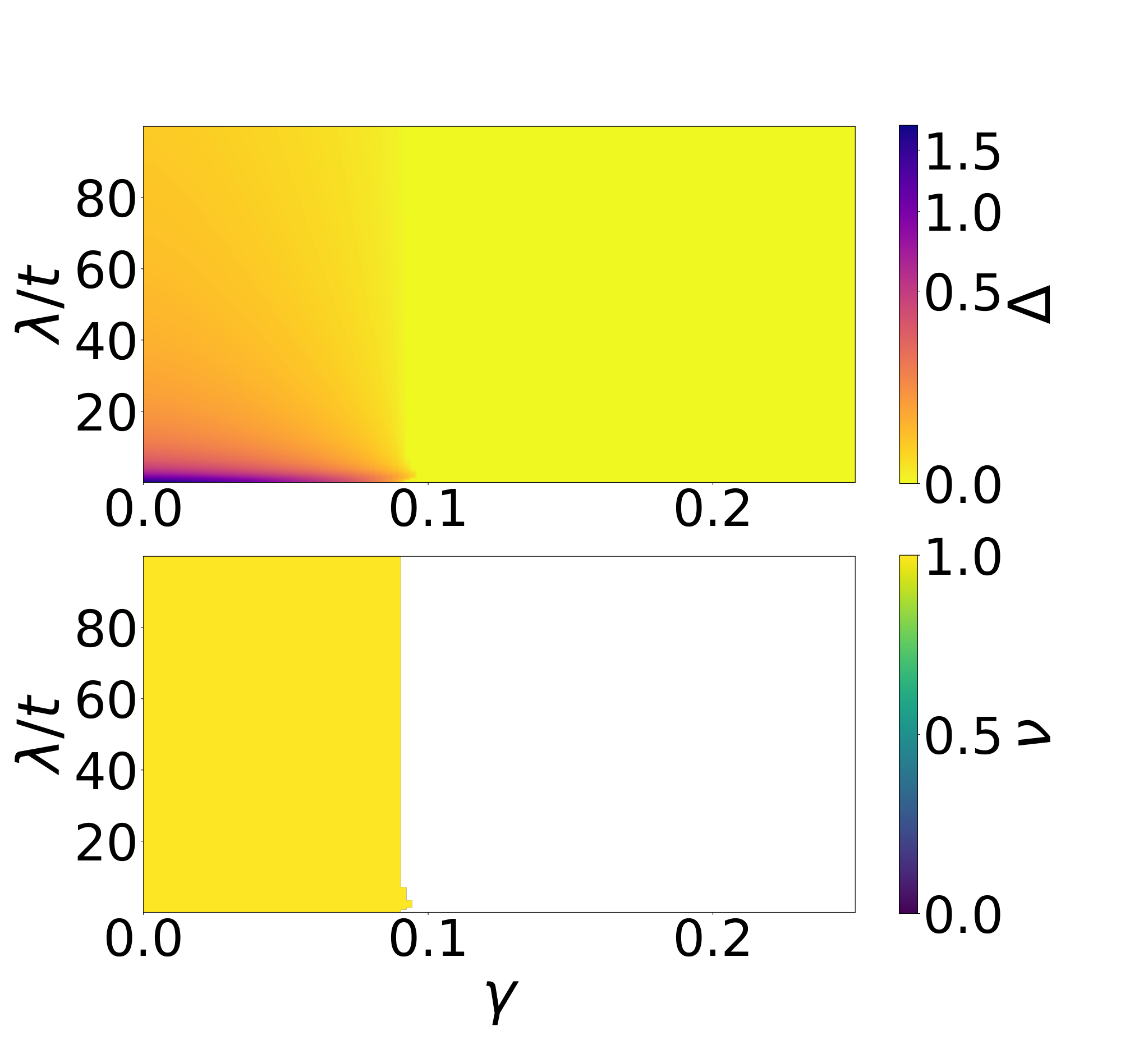
V.2 On-site energies applied in $R$ -sublattice sites: ${\lambda_{R,1}=-\lambda_{R,2}=\lambda}$ and $\lambda_{B,s=1,2}=\lambda_{G,s=1,2}=0$

Here, we study the behavior of the system when a finite on-site energy is applied in one of the sublattice sites only. We present our results for filling $n=2/3$ . We consider the flux $\phi=\pi/2$ and on-site energies ${\lambda_{R,1}=-\lambda_{R,2}=\lambda}$ and $\lambda_{B,s=1,2}=\lambda_{G,s=1,2}=0$ . We observe only one gapped phase which also exists for very large values of $\lambda$ . We check this numerically up to $\lambda=100t$ . Our results are presented in Fig. 15. By calculating the $\mathbb{Z}_{2}$ number we obtain that the gapped phase is a topological insulator. Again for this setup, we obtain a topological phase in the limit $\lambda\rightarrow\infty$ .

We also perform calculations for other values of $\phi$ (not shown) and we obtain a similar phase diagram.

VI Conclusions

In this work, we have studied topological properties of the spin-orbit coupled time-reversal tight-binding model with flux on the Kagome lattice. In addition to the spin-orbit coupling $\gamma$ and the flux $\phi$ , we also considered the effect of the on-site energies $V_{\alpha,{\bf r}}$ . First, we considered the case where the on-site energies are independent of the spatial coordinate $\bf r$ but differ within the unit cell, i.e., $V_{\alpha,{\bf r}}=\lambda_{\alpha}$ . In this case, we obtain that the system has three bands that are potentially non-overlapping for any value of $\bf k$ . It follows that for filling situations $n=2/3$ and $n=4/3$ a gapped phase can occur. Because of the symmetries of our model, the results for these two fillings are related by Eq. (48). Here we have presented results for the the filling $n=2/3$ . We also performed calculations for a staggered potential. For the latter we have $V_{\alpha,{\bf r}}=\lambda_{\alpha,1}$ for ${\bf r}=2n_{1}{\bf e}_{1}+n_{2}{\bf e}_{2}$ and $V_{\alpha,{\bf r}}=\lambda_{\alpha,2}$ for ${\bf r}=(2n_{1}+1){\bf e}_{1}+n_{2}{\bf e}_{2}$ . In this case, we obtain that the system has six potentially non-overlapping bands for all values of $\bf k$ . It follows that a gapped phase can occur for fillings $n=1/3$ , $n=2/3$ , $n=1$ , $n=4/3$ , and $n=5/3$ . In this work we have presented results for $n=2/3$ and for half-filling $n=1$ .

The model has time-reversal symmetry, and to determine its topological nature we calculated the $\mathbb{Z}_{2}$ invariant. For this purpose, we used three methods. One of them is numerical and based on the twisted boundary conditionsFukui, Hatsugai, and Suzuki 2005; Fukui and Hatsugai 2007; Kumar, Mertz, and Hofstetter 2016; Irsigler et al. 2020, while the other two are analytical. One of them introduces different smooth fields for several domains in the reciprocal space and was developed by us. The phase accumulated at the boundary between the smooth fields’ domains is related to the topological properties. It is important to remind that such a smooth fields approach has recently been shown to be useful on the honeycomb lattice, e.g., to indicate that transport and light-matter properties can be revealed from the Dirac points onlyKlein, Grushin, and Le Hur 2021; Hutchinson and Hur 2020.

The other approach described in Appendix A.1 is along the line of the method introduced on the honeycomb lattice for $\mathbb{Z}_{2}$ topological insulatorsKane and Mele 2005a; Kane and Mele 2005b; Fu and Kane 2007. We also aimed at developing the "counting points" method in an energy band, as discussed previously in Ref. Petrescu, Houck, and Le Hur 2012. Here, we observe gap closing effects when $\gamma\neq 0$ such that the results must be taken with care in that situation; see Appendix A.2.

Depending on the model parameters, we obtain the topological insulator, the trivial band insulator, and the metallic phase. We show that the obtained topological phases are stable after applying on-site energies. Even more, if the flat band for half-filling is split due to the the staggered potential in combination with flux and spin-orbit coupling, stable topological phases appear for arbitrarily small gap sizes.

One of the most interesting results we obtain is the existence of the topological phase for infinitely large on-site energies. We show that for selected sets of parameters, in particular when on-site energies were applied only on one of the sublattice sides for $n=2/3$ , we obtain a topological insulator for infinitely large on-site energies.

The situations with finite on-site energies were studied previously related to topological insulators. In the original paper by Kane and Mele, the effect of a finite staggered potential was already consideredKane and Mele 2005a; Kane and Mele 2005b. Topological phases were obtained for finite on-site energies, while for large on-site energies, the system was shown to be topologically trivial. Recently, a topological phase for infinitely large on-site energies was observed for a mixture of three component fermions, on a triangular lattice at $1/3$ filling, in the presence of a gauge potential stabilizing a quantum Hall insulatorHafez-Torbati et al. 2020.

Experimental progress in ultracold atomic gases allows to realize and study such systems. Topological phases have already been realized by loading ultracold atoms in optical latticesAidelsburger et al. 2013; Aidelsburger et al. 2015; Miyake et al. 2013; Jotzu et al. 2014; Fläschner et al. 2016; Mancini et al. 2015; Stuhl et al. 2015. For this purpose, artificial gauge fieldsGerbier and Dalibard 2010; Dalibard et al. 2011; Goldman and Dalibard 2014; Goldman et al. 2014; Goldman, Budich, and Zoller 2016; Galitski, Juzeliūnas, and Spielman 2019; Galitski and Spielman 2013 were used. In particular, ultracold atomic gases also allow the realization of SOCLin, Jiménez-García, and Spielman 2011; Wang et al. 2012; Cheuk et al. 2012; Huang et al. 2016. As mentioned above, the Kagome lattice can be realized experimentally by superimposing two optical triangular lattices with different wavelengths.Jo et al. 2012 The experimental realization of periodically oscillating on-site energies, i.e. superlattices, is also well establishedGuidoni and Verkerk 1998; Ritt et al. 2006; Sebby-Strabley et al. 2006; Fölling et al. 2007; Cheinet et al. 2008; Gerbier and Dalibard 2010; Lang, Cai, and Chen 2012; Nascimbène et al. 2012. The physics obtained in this paper can be observed for systems cooled down to temperatures $T<\Delta/k_{B}$ , as the gap $\Delta$ is of the order of $t$ and the typical hopping amplitude for ultracold atomic gases is of the order $0.1$ kHzBloch, Dalibard, and Zwerger 2008, the system must reach temperatures of the order of $1$ nK. In real materials $\phi\leq\pi/4$ and spin-orbit coupling is always smaller compared to the hopping amplitude between corresponding nearest neighbors, which in our notations means that $\gamma\leq 1/4$ .Manchon et al. 2015; Wang et al. 2018; Wang et al. 2016 Ultracold atomic gases allow to consider larger intervals of Peierls phase $\phi$ . The maximal value of the Peierls phase which can be obtained is $\phi=\pi/2$ while $\gamma\leq 1/4$ .Stanescu, Galitski, and Das Sarma 2010; Goldman et al. 2010 We conclude that the results obtained in our work may be very relevant for upcoming experiments.

Acknowledgements.

This work was supported by the Deutsche Forschungsgemeinschaft (DFG, German Research Foundation) under Project No. 277974659 via Research Unit FOR 2414. This work was also supported by the DFG via the high performance computing center Goethe-HLR. The research on the topological Kagome lattice is also funded by ANR BOCA (KLH) for which JL is also supported for his PhD.

Appendix A Two other ways of computing the $\mathbb{Z}_{2}$ number at $\gamma=0$ .

$\lambda$	$(n_{1},n_{2})$	Eigenvalues $E_{l}$	Eigenvector’s coefficient $\left(r_{\sigma}({\bf k}),b_{\sigma}({\bf k}),g_{\sigma}({\bf k})\right)$	Parity operator	$(-1)^{\nu}$
$\lambda<-\sqrt{2}t$	$(1,0)$	$\lambda$	$(0,t,0)$	diag $(1,-1,1)$	$+1$
	$(0,1)$	$-\sqrt{4t^{2}+\lambda^{2}}$	$(-2t^{2}/\left(\lambda+E_{l}\right),t,0)$	diag $(1,1,-1)$
	$(1,1)$	$\left(\lambda-\sqrt{16t^{2}+\lambda^{2}}\right)/2$	$(0,2t^{2}\textrm{e}^{is_{z}\phi}/\left(\lambda-E_{l}\right),t)$	diag $(1,-1,-1)$
$-\sqrt{2}t<\lambda<\sqrt{2}t$	$(1,0)$	$-\left(\lambda+\sqrt{16t^{2}+\lambda^{2}}\right)/2$	$(-2t^{2}/\left(\lambda+E_{l}\right),0,t)$	diag $(1,-1,1)$	$-1$
	$(0,1)$	$-\sqrt{4t^{2}+\lambda^{2}}$	$(-2t^{2}/\left(\lambda+E_{l}\right),t,0)$	diag $(1,1,-1)$
	$(1,1)$	$\left(\lambda-\sqrt{16t^{2}+\lambda^{2}}\right)/2$	$(0,2t^{2}\textrm{e}^{is_{z}\phi}/\left(\lambda-E_{l}\right),t)$	diag $(1,-1,-1)$
$\lambda>\sqrt{2}t$	$(1,0)$	$-\left(\lambda+\sqrt{16t^{2}+\lambda^{2}}\right)/2$	$(-2t^{2}/\left(\lambda+E_{l}\right),0,t)$	diag $(1,-1,1)$	$+1$
	$(0,1)$	$-\sqrt{4t^{2}+\lambda^{2}}$	$(-2t^{2}/\left(\lambda+E_{l}\right),t,0)$	diag $(1,1,-1)$
	$(1,1)$	$-\lambda$	$(t,0,0)$	diag $(1,-1,-1)$

Table 1: Table resuming the computation of the

Z_{2}

topological invariant

\nu

for an inversion and time-reversal symmetric system. In this example, we took the chemical potentials to be

\lambda_{B}=-\lambda_{R}=\lambda

and

\lambda_{G}=0

. For definition

(n_{1},n_{2})

see Eq. (109), while for definitions

\left(r_{\sigma}({\bf k}),b_{\sigma}({\bf k}),g_{\sigma}({\bf k})\right)

see Sec. IV.2.2

$\lambda$	$(n_{1},n_{2})$	Eigenvalues $E_{l}$	Eigenvector’s coefficient $\left(r_{\sigma}({\bf k}),b_{\sigma}({\bf k}),g_{\sigma}({\bf k})\right)$	Parity operator	$(-1)^{\nu}$
$\lambda<-2t$	$(1,0)$	$\left(\lambda-\sqrt{16t^{2}+\lambda^{2}}\right)/2$	$(-E_{l}/2,0,t)$	diag $(1,-1,1)$	$+1$
	$(0,1)$	$\left(\lambda-\sqrt{16t^{2}+\lambda^{2}}\right)/2$	$(-E_{l}/2,t,0)$	diag $(1,1,-1)$
	$(1,1)$	$\lambda$	$(t,0,0)$	diag $(1,-1,-1)$
$\lambda>-2t$	$(1,0)$	$\left(\lambda-\sqrt{16t^{2}+\lambda^{2}}\right)/2$	$(-E_{l}/2,0,t)$	diag $(1,-1,1)$	$-1$
	$(0,1)$	$\left(\lambda-\sqrt{16t^{2}+\lambda^{2}}\right)/2$	$(-E_{l}/2,t,0)$	diag $(1,1,-1)$
	$(1,1)$	$-2t$	$(0,-t\textrm{e}^{is_{z}\phi},1)$	diag $(1,-1,-1)$

Table 2: Table resuming the computation of the

Z_{2}

topological invariant

\nu

for an inversion and time-reversal symmetric system. In this example, we took the chemical potentials to be

\lambda_{R}=\lambda

and

\lambda_{B}=\lambda_{G}=0

. For definition

(n_{1},n_{2})

see Eq. (109), while for definitions

\left(r_{\sigma}({\bf k}),b_{\sigma}({\bf k}),g_{\sigma}({\bf k})\right)

see Sec. IV.3.2

A.1 Using inversion symmetry.

When our system is inversion symmetric (i.e. $\gamma=0$ ), the $\mathbb{Z}_{2}$ topological invariant $\nu$ (defined for time-reversal invariant Hamiltonian, i.e. $B=0$ ) is given byFu and Kane 2007

(-1)^{\nu}=\prod_{\begin{subarray}{c}n_{1}=0,1\\ n_{2}=0,1\end{subarray}}\delta_{(n_{1},n_{2})}

(108)

with $\delta_{(n_{1},n_{2})}=\prod_{m=1}^{N}p_{2m}\left(\Gamma_{(n_{1},n_{2})}\right)$ is the product of the parity eigenvalues $p_{2m}$ , at $\Gamma_{(n_{1},n_{2})}$ , associated to each occupied Kramers’ degenerate pair ( $p_{2m}$ and $p_{2m-1}$ are identical). The $\Gamma_{(n_{1},n_{2})}$ points are the time-reversal invariant points, i.e. the points such that $H(\Gamma_{(n_{1},n_{2})})=\Theta H(\Gamma_{(n_{1},n_{2})})\Theta^{-1}$ . These points can be written

\Gamma_{(n_{1},n_{2})}=\dfrac{1}{2}\left(n_{1}\boldsymbol{g}_{1}+n_{2}\boldsymbol{g}_{2}\right),

(109)

with $\boldsymbol{g}_{1}$ and $\boldsymbol{g}_{2}$ both reciprocal lattice basis vectors. These points correspond to the so-called $\bf\Gamma$ point and to the three $\bf M$ points.

We find the parity eigenvalues $p_{2m}$ associated to each of the four $\Gamma_{(n_{1},n_{2})}$ points. We need to express the Hamiltonian and the momentum space parity operator at these points. When $\gamma=0$ , the Hamiltonian decouples into two independent parts, and it gives 3 energy bands associated to the spin up states, which are degenerated with the 3 energy bands associated to the spin down states. At $n=2/3$ filling, a Kramers’ degenerate pair is occupied. This pair contains the lowest energy band associated to each spin species. Formula 108 only implies the parity eigenvalues associated to one band, because the ones associated to the other band are identical. Therefore, in the following, we consider separately each of both diagonal parts of the Hamiltonian 3.

The parity operator can be defined in real space by

P\left(c_{R,\boldsymbol{r}},c_{B,\boldsymbol{r}},c_{G,\boldsymbol{r}}\right)=\left(c_{R,-\boldsymbol{r}},c_{B,-\boldsymbol{r}-\boldsymbol{e}_{1}},c_{G,-\boldsymbol{r}-\boldsymbol{e}_{2}}\right).

(110)

A Fourier transformation of the fermionic operators enables to see that, in momentum space, the parity operator reads

P_{{\bf k}}=\textrm{diag}\left(1,\textrm{e}^{-i\boldsymbol{e}_{1}{\bf k}},\textrm{e}^{-i\boldsymbol{e}_{2}{\bf k}}\right).

(111)

Therefore, at the ${\bf\Gamma}_{(0,0)}$ point, $P_{\boldsymbol{\Gamma}_{(0,0)}}$ is diagonal so $\delta_{{(0,0)}}=1$ and at the other points we have ${P_{\boldsymbol{\Gamma}_{(1,0)}}=\textrm{diag}\left(1,-1,1\right)}$ , ${P_{\boldsymbol{\Gamma}_{(0,1)}}=\textrm{diag}\left(1,1,-1\right)}$ , and ${P_{\boldsymbol{\Gamma}_{(1,1)}}=\textrm{diag}\left(1,-1,-1\right)}$ .

Now we need to evaluate the lowest energy associated eigenvectors of ${\cal H}_{\uparrow}({\bf k})$ at $\boldsymbol{\Gamma}_{(1,0)}$ , $\boldsymbol{\Gamma}_{(0,1)}$ , and $\boldsymbol{\Gamma}_{(1,1)}$ . We consider two different setups $\lambda_{B}=-\lambda_{R}=\lambda$ and $\lambda_{G}=0$ or $\lambda_{R}=\lambda$ and $\lambda_{B}=\lambda_{G}=0$ . We start with $\lambda_{B}=-\lambda_{R}=\lambda$ and $\lambda_{G}=0$ . We denote the lowest energy eigenvalue $E_{l}({\bf k})$ and we write $\ket{u_{\sigma,{\bf k}}}$ the $\sigma$ spin species associated eigenvector

\ket{u_{\sigma,{\bf k}}}=\dfrac{\left(r_{\sigma}({\bf k})c_{R,{\bf k},\sigma}^{\dagger}+b_{\sigma}({\bf k})c_{B,{\bf k},\sigma}^{\dagger}+g_{\sigma}({\bf k})c_{G,{\bf k},\sigma}^{\dagger}\right)\ket{0}}{\sqrt{\left|r_{\sigma}({\bf k})\right|^{2}+\left|b_{\sigma}({\bf k})\right|^{2}+\left|g_{\sigma}({\bf k})\right|^{2}}}\,.

(112)

We notice that

•

at the $\boldsymbol{\Gamma}_{(1,0)}$ point, for $\lambda<-\sqrt{2}t$ , the smallest eigenvalue is ${E_{l}=\lambda}$ and the associated eigenvector is proportional to $(0,1,0)$ , while for ${\lambda>-\sqrt{2}t}$ , the smallest eigenvalue is ${E_{l}=-\left(\lambda+\sqrt{16t^{2}+\lambda^{2}}\right)/2}$ , with associated eigenvector proportional to $(-2t/\left(\lambda+E_{l}\right),0,1)$ .
•

at the $\boldsymbol{\Gamma}_{(0,1)}$ point, the smallest eigenvalue is ${E_{l}=-\sqrt{4t^{2}+\lambda^{2}}}$ and the eigenvector associated to it is proportional to $(-2t/\left(\lambda+E_{l}\right),1,0)$ .
•

at the $\boldsymbol{\Gamma}_{(1,1)}$ point, if $\lambda>\sqrt{2}t$ , then ${E_{l}=-\lambda}$ is the smallest eigenvalue and the associated eigenvector is proportional to $(1,0,0)$ , while if $\lambda<\sqrt{2}t$ , then the smallest eigenvalue is ${E_{l}=\left(\lambda-\sqrt{16t^{2}+\lambda^{2}}\right)/2}$ , with associated eigenvector proportional to $(0,2t\textrm{e}^{is_{z}\phi}/\left(\lambda-E_{l}\right),1)$ .

Applying the parity operator and the eigenvectors, we find that the phases $\lambda>\sqrt{2}t$ and $\lambda<-\sqrt{2}t$ are trivial insulators while the phase $-\sqrt{2}t<\lambda<\sqrt{2}t$ is a topological insulator. These results are sum up in table 1.

Now we consider $\lambda_{R}=\lambda$ and $\lambda_{B}=\lambda_{G}=0$ . We notice that

•

at the $\boldsymbol{\Gamma}_{(1,0)}$ point, the smallest eigenvalue is ${E_{l}=\left(\lambda-\sqrt{16t^{2}+\lambda^{2}}\right)/2}$ , with associated eigenvector proportional to $(-E_{l}/2t,0,1)$ .
•

at the $\boldsymbol{\Gamma}_{(0,1)}$ point, the smallest eigenvalue is ${E_{l}=\left(\lambda-\sqrt{16t^{2}+\lambda^{2}}\right)/2}$ , with associated eigenvector proportional to $(-E_{l}/2t,1,0)$ .
•

at the $\boldsymbol{\Gamma}_{(1,1)}$ point, if $\lambda<-2t$ , then $E_{l}=\lambda$ is the smallest eigenvalue and the associated eigenvector is proportional to $(1,0,0)$ , while if $\lambda>-2t$ , then the smallest eigenvalue is $E_{l}=-2t$ , with associated eigenvector proportional to $(0,-\textrm{e}^{is_{z}\phi},1)$ .

Applying the parity operator on the eigenvectors, we find that the phase $\lambda<-2t$ is a trivial insulator while the phase $\lambda>-2t$ is a topological insulator. These results are sum up in Table 2.

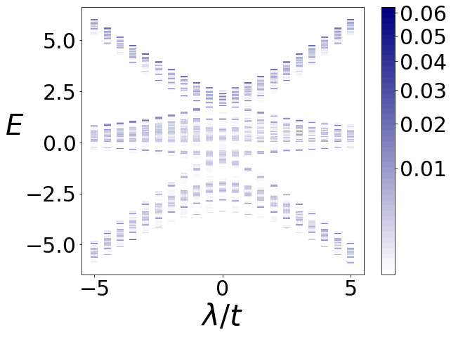
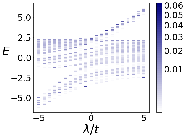
A.2 Counting the subband number under a weak magnetic field.

Here we consider the case $V_{\alpha,{\bf r}}=\lambda_{\alpha}$ , $\gamma=0$ . We review another method to determine the Chern number associated to the energy bands of our model. It is based on the numerical determination of the energy spectrum when we add a weak magnetic field $\boldsymbol{\cal B}={\cal B}\hat{\boldsymbol{z}}$ orthogonal to the Kagome lattice plane. That is we add the term

-{\cal B}\sum_{\bf r}\sum_{\alpha=R,B,G}\left(n_{\alpha,{\bf r},\uparrow}-n_{\alpha,{\bf r},\downarrow}\right)

(113)

in the Hamiltonian and also an extra coordinate dependent flux $\phi_{1}({\bf r})$ for the hopping between nearest neighbor sites.

As we argue before, the Hamiltonian decouples into two spin independent parts. Spin up and spin down part are associated to opposite energy bands’ Chern number. Here for simplicity, we only consider the spin up part of the Hamiltonian. We call the energy bands when ${{\cal B}=0}$ the "parents bands". Under a weak magnetic field, each parent band $i$ is spitted into a certain number of subband that we denote $D_{i}$ . We can link this number to the amplitude of the magnetic field and to the Chern number $\nu_{i}$ of the $i^{th}$ parent bandChang and Niu 1995; Petrescu, Houck, and Le Hur 2012. We introduce $f=qn_{\phi}$ where $n_{\phi}=\dfrac{{\cal B}a^{2}}{h/e}$ is the number of flux quanta in the system and $q$ is the area of the first magnetic Brillouin zone. In the following, we choose $\cal B$ such that $1/f$ is an integer. Then we have:

\nu_{i}=\dfrac{1}{f}-D_{i}.

(114)

First we show that this method is useful at $\lambda_{\alpha}=0$ , $\alpha={R,B,G}$ , or $\lambda_{\alpha}\ll t$ . We implement the effect of the $\cal B$ field in the Hamiltonian. We compute the energy spectrum and the energy density of states (DoS) so that we can count the number of subbands arising from each parent band. We consider for instance $1/f=5$ . Figure 16 show the density of states (DoS) at different values $\lambda_{\alpha}$ . At $\lambda_{\alpha}=0,\,\alpha=R,B,G$ , we see that we have $D_{1}=4$ subbands, $D_{2}=5$ subbands and $D_{3}=6$ subbands, which gives $\nu_{1}=-\nu_{3}=1$ , and $\nu_{2}=0$ . We see that when $|\lambda_{\alpha}|$ start increasing, counting the subbands is becoming more and more difficult; when $\lambda_{\alpha}$ reaches a value of the order $t$ or greater, the determination of the Chern number relying on this method becomes impracticable.

When $\gamma\neq 0$ , several issues prevent us from extending this method to compute the energy bands’ Chern number. First, the Hamiltonian does not decouple into two spin independent parts. Formula 114, relies on a semiclassical dynamics description of the Bloch electrons in a magnetic field with no interband tunneling. At $\gamma\neq 0$ , this description is much more tricky to draw because the bands are crossing. Moreover, we can not identify the subbands arising from each parent band, so counting the former is impracticable.

Appendix B Conservation of the average current along ${\cal E}_{2}$ direction

Here we compute the time derivative of the average value of the current operator for one directional line, that we denote ${\cal E}_{2}$ , along the ${\bf e}_{2}$ direction. We remind that we consider an inversion symmetric lattice with line-shape boundaries. The ${\cal E}_{2}$ line crosses a certain number of unit cells and may have 2 extremities if the system is open in the ${\bf e}_{2}$ direction. Both atoms at the extremity of the line have the same color that we denote $\alpha_{e}$ , $\alpha_{e}=R$ or $G$ . For each unit cell at position ${\bf r}$ , we need to consider the currents along ${\cal E}_{2}$ , which are ${\bf j}_{(G,{\bf r}),(R,{\bf r})}(\tau)$ and ${\bf j}_{(R,{\bf r}+{\bf e}_{2}),(G,{\bf r})}(\tau)$ . We have

$\displaystyle\left[{\cal H}(\tau),{\bf j}_{(G,{\bf r}),(R,{\bf r})}(\tau)\right]$	$\displaystyle=$	$\displaystyle-{\bf e}_{2}\left[it^{2}\left(\sin^{2}\tau-\cos^{2}\tau\right)\sum_{\sigma=\{\uparrow,\downarrow\}}\left[\left(c_{R,{\bf r}+{\bf e}_{2},\sigma}^{\dagger}c_{R,{\bf r},\sigma}^{\phantom{\dagger}}-c_{G,{\bf r}-{\bf e}_{2},\sigma}^{\dagger}c_{G,{\bf r},\sigma}^{\phantom{\dagger}}\right)+H.c.\right]\right.$	(115)
	$\displaystyle+$	$\displaystyle it^{2}\cos\tau\sum_{\sigma=\{\uparrow,\downarrow\}}\left[\left(c_{G,{\bf r},\sigma}^{\dagger}c_{B,{\bf r},\sigma}^{\phantom{\dagger}}+c_{G,{\bf r},\sigma}^{\dagger}c_{B,{\bf r}-{\bf e}_{1},\sigma}^{\phantom{\dagger}}\right)+H.c.\right]$
	$\displaystyle-$	$\displaystyle it^{2}\cos\tau\sum_{\sigma=\{\uparrow,\downarrow\}}\left[\left(e^{is_{z}\phi}c_{B,{\bf r},\sigma}^{\dagger}c_{R,{\bf r},\sigma}^{\phantom{\dagger}}+e^{is_{z}\phi}c_{B,{\bf r}+{\bf e}_{3},\sigma}^{\dagger}c_{R,{\bf r},\sigma}^{\phantom{\dagger}}\right)+H.c.\right]$
	$\displaystyle+$	$\displaystyle 2it^{2}\cos^{2}\tau\sum_{\sigma=\{\uparrow,\downarrow\}}\left(c_{G,{\bf r},\sigma}^{\dagger}c_{G,{\bf r},\sigma}^{\phantom{\dagger}}-c_{R,{\bf r},\sigma}^{\dagger}c_{R,{\bf r},\sigma}^{\phantom{\dagger}}\right)$
	$\displaystyle+$	$\displaystyle 2t^{2}\cos\tau\sin\tau\sum_{\sigma=\{\uparrow,\downarrow\}}\left(c_{R,{\bf r}+{\bf e}_{2},\sigma}^{\dagger}c_{R,{\bf r},\overline{\sigma}}^{\phantom{\dagger}}+c_{G,{\bf r}-{\bf e}_{2},\sigma}^{\dagger}c_{G,{\bf r},\sigma}^{\phantom{\dagger}}\right)-H.c.$
	$\displaystyle-$	$\displaystyle t^{2}\sin\tau\sum_{\sigma=\{\uparrow,\downarrow\}}\left(c_{G,{\bf r},\sigma}^{\dagger}c_{B,{\bf r},\overline{\sigma}}^{\phantom{\dagger}}+c_{G,{\bf r},\sigma}^{\dagger}c_{B,{\bf r}-{\bf e}_{1},\overline{\sigma}}^{\phantom{\dagger}}\right)-H.c.$
	$\displaystyle+$	$\displaystyle\left.t^{2}\sin\tau\sum_{\sigma=\{\uparrow,\downarrow\}}\left(e^{is_{z}(\sigma)\phi}c_{B,{\bf r},\sigma}^{\dagger}c_{R,{\bf r},\overline{\sigma}}^{\phantom{\dagger}}+e^{is_{z}(\sigma)\phi}c_{B,{\bf r}+{\bf e}_{3},\sigma}^{\dagger}c_{R,{\bf r},\overline{\sigma}}^{\phantom{\dagger}}\right)-H.c.\right]$

\dfrac{d}{d\tau}{\bf j}_{(G,{\bf r}),(R,{\bf r})}(\tau)={\bf e}_{2}\,\,t\sum_{\sigma=\{\uparrow,\downarrow\}}\left(i\sin\tau\,c_{G,{\bf r},\sigma}^{\dagger}c_{R,{\bf r},\sigma}^{\phantom{\dagger}}+\cos\tau\,c_{G,{\bf r},\sigma}^{\dagger}c_{R,{\bf r},\overline{\sigma}}^{\phantom{\dagger}}\right)+H.c.\,,

(116)

$\displaystyle\left[{\cal H}(\tau),{\bf j}_{(R,{\bf r}+{\bf e}_{2}),(G,{\bf r})}(\tau)\right]$	$\displaystyle=$	$\displaystyle-{\bf e}_{2}\left[it^{2}\left(\cos^{2}\tau-\sin^{2}\tau\right)\sum_{\sigma=\{\uparrow,\downarrow\}}\left[\left(c_{R,{\bf r}+{\bf e}_{2},\sigma}^{\dagger}c_{R,{\bf r},\sigma}^{\phantom{\dagger}}-c_{G,{\bf r}+{\bf e}_{2},\sigma}^{\dagger}c_{G,{\bf r},\sigma}^{\phantom{\dagger}}\right)+H.c.\right]\right.$	(117)
	$\displaystyle-$	$\displaystyle it^{2}\cos\tau\sum_{\sigma=\{\uparrow,\downarrow\}}\left[\left(c_{G,{\bf r},\sigma}^{\dagger}c_{B,{\bf r}+{\bf e}_{3},\sigma}^{\phantom{\dagger}}+c_{G,{\bf r},\sigma}^{\dagger}c_{B,{\bf r}+{\bf e}_{2},\sigma}^{\phantom{\dagger}}\right)+H.c.\right]$
	$\displaystyle+$	$\displaystyle it^{2}\cos\tau\sum_{\sigma=\{\uparrow,\downarrow\}}\left[\left(e^{is_{z}\phi}c_{B,{\bf r},\sigma}^{\dagger}c_{R,{\bf r}+{\bf e}_{2},\sigma}^{\phantom{\dagger}}+e^{is_{z}\phi}c_{B,{\bf r}+{\bf e}_{3},\sigma}^{\dagger}c_{R,{\bf r}+{\bf e}_{2},\sigma}^{\phantom{\dagger}}\right)+H.c.\right]$
	$\displaystyle+$	$\displaystyle 2it^{2}\cos^{2}\tau\sum_{\sigma=\{\uparrow,\downarrow\}}\left(c_{R,{\bf r}+{\bf e}_{2},\sigma}^{\dagger}c_{R,{\bf r}+{\bf e}_{2},\sigma}^{\phantom{\dagger}}-c_{G,{\bf r},\sigma}^{\dagger}c_{G,{\bf r},\sigma}^{\phantom{\dagger}}\right)$
	$\displaystyle-$	$\displaystyle 2t^{2}\cos\tau\sin\tau\sum_{\sigma=\{\uparrow,\downarrow\}}\left(c_{R,{\bf r}+{\bf e}_{2},\sigma}^{\dagger}c_{R,{\bf r},\overline{\sigma}}^{\phantom{\dagger}}-c_{G,{\bf r}+{\bf e}_{2},\sigma}^{\dagger}c_{G,{\bf r},\sigma}^{\phantom{\dagger}}\right)-H.c.$
	$\displaystyle-$	$\displaystyle t^{2}\sin\tau\sum_{\sigma=\{\uparrow,\downarrow\}}\left(c_{G,{\bf r},\sigma}^{\dagger}c_{B,{\bf r}+{\bf e}_{3},\overline{\sigma}}^{\phantom{\dagger}}+c_{G,{\bf r},\sigma}^{\dagger}c_{B,{\bf r}+{\bf e}_{2},\overline{\sigma}}^{\phantom{\dagger}}\right)-H.c.$
	$\displaystyle+$	$\displaystyle\left.t^{2}\sin\tau\sum_{\sigma=\{\uparrow,\downarrow\}}\left(e^{is_{z}(\sigma)\phi}c_{B,{\bf r},\sigma}^{\dagger}c_{R,{\bf r}+{\bf e}_{2},\overline{\sigma}}^{\phantom{\dagger}}+e^{is_{z}(\sigma)\phi}c_{B,{\bf r}+{\bf e}_{3},\sigma}^{\dagger}c_{R,{\bf r}+{\bf e}_{2},\overline{\sigma}}^{\phantom{\dagger}}\right)-H.c.\right]\,,$

and

\dfrac{d}{d\tau}{\bf j}_{(R,{\bf r}+{\bf e}_{2}),(G,{\bf r})}(\tau)={\bf e}_{2}\,\,t\sum_{\sigma=\{\uparrow,\downarrow\}}\left(i\sin\tau\,c_{G,{\bf r},\sigma}^{\dagger}c_{R,{\bf r}+{\bf e}_{2},\sigma}^{\phantom{\dagger}}+\cos\tau\,c_{G,{\bf r},\sigma}^{\dagger}c_{R,{\bf r}+{\bf e}_{2},\overline{\sigma}}^{\phantom{\dagger}}\right)+H.c.,

(118)

We can notice that, integrated along the whole line ${\cal E}_{2}$ , the $1^{\textrm{st}}$ and the $5^{\textrm{th}}$ terms of the commutator 115 are canceled by the ones of the commutator 117, and the $4^{\textrm{th}}$ term of both commutators give a resulting contribution $2it^{2}\cos^{2}\tau\sum_{\sigma=\{\uparrow,\downarrow\}}\left(c_{\alpha_{e},{\bf r}_{1},\sigma}^{\dagger}c_{\alpha_{e},{\bf r}_{1},\sigma}^{\phantom{\dagger}}-c_{\alpha_{e},{\bf r}_{2},\sigma}^{\dagger}c_{\alpha_{e},{\bf r}_{2},\sigma}^{\phantom{\dagger}}\right)$ , with ${\bf r}_{1}$ and ${\bf r}_{2}$ both positions at the extremity of ${\cal E}_{2}$ . Moreover, we notice that the Hamiltonian is invariant under inversion symmetry added to the transformation $\gamma\rightarrow-\gamma$ . This transforms the $2^{\textrm{nd}}$ , $3^{\textrm{rd}}$ , $6^{\textrm{th}}$ and $7^{\textrm{th}}$ terms in the commutator 115 (taken at some position ${\bf r}$ ) respectively into the opposite of the same terms in the commutator 117 (taken at the inversion symmetric position ${\bf r}_{R}$ ) and the term $2it^{2}\cos^{2}\tau\sum_{\sigma=\{\uparrow,\downarrow\}}\left(c_{\alpha_{e},{\bf r}_{1},\sigma}^{\dagger}c_{\alpha_{e},{\bf r}_{1},\sigma}^{\phantom{\dagger}}-c_{\alpha_{e},{\bf r}_{2},\sigma}^{\dagger}c_{\alpha_{e},{\bf r}_{2},\sigma}^{\phantom{\dagger}}\right)$ into its opposite, while it leaves the terms 116 and 118 unchanged. It means that we have

	$\displaystyle\sum_{{\bf r}\in\mathcal{E}_{2}}\bra{\Psi(\tau)}\left(\dfrac{i}{\hbar}\left[{\cal H}(\tau),{\bf j}_{(G,{\bf r}),(R,{\bf r})}(\tau)\right]+\dfrac{i}{\hbar}\left[{\cal H}(\tau),{\bf j}_{(R,{\bf r}+{\bf e}_{2}),(G,{\bf r})}(\tau)\right]\right)\ket{\Psi(\tau)}$
	$\displaystyle=\sum_{{\bf r}\in\mathcal{E}_{2}}\bra{\Psi(\tau)}\left(-\dfrac{i}{\hbar}\left[{\cal H}(\tau),{\bf j}_{(R,{\bf r}+{\bf e}_{2}),(G,{\bf r})}(\tau)\right]-\dfrac{i}{\hbar}\left[{\cal H}(\tau),{\bf j}_{(G,{\bf r}),(R,{\bf r})}(\tau)\right]\right)\ket{\Psi(\tau)},$

where $\mathcal{E}_{2}$ is the ensemble containing the positions of all the unit cells belonging to the ${\cal E}_{2}$ line. From this we deduce that the term

	$\displaystyle\hskip-49.79231pt\sum_{{\bf r}\in\mathcal{E}_{2}}\bra{\Psi(\tau)}\Biggl(\dfrac{i}{\hbar}\left[{\cal H}(\tau),{\bf j}_{(G,{\bf r}),(R,{\bf r})}(\tau)\right]$
	$\displaystyle+\dfrac{i}{\hbar}\left[{\cal H}(\tau),{\bf j}_{(R,{\bf r}+{\bf e}_{2}),(G,{\bf r})}(\tau)\right]\Biggl)\ket{\Psi(\tau)}$

amounts to a vanishing contribution.

The Hamiltonian is also invariant under ${c_{\alpha,{\bf r}}^{\dagger}=\left(c_{\alpha,{\bf r},\uparrow}^{\dagger},c_{\alpha,{\bf r},\downarrow}^{\dagger}\right)\rightarrow c_{\alpha,{\bf r}}^{\dagger\,\prime}=\left(-c_{\alpha,{\bf r},\uparrow}^{\dagger},c_{\alpha,{\bf r},\downarrow}^{\dagger}\right),}$ ${\alpha=R\,,\,B\,,\,G}$ , added to the transformation $\gamma\rightarrow-\gamma$ . From this we deduce that each of the operators $\bra{\Psi(\tau)}\left(\dfrac{d}{d\tau}{\bf j}_{(G,{\bf r}),(R,{\bf r})}(\tau)\right)\ket{\Psi(\tau)}$ and $\bra{\Psi(\tau)}\left(\dfrac{d}{d\tau}{\bf j}_{(R,{\bf r}+{\bf e}_{2}),(G,{\bf r})}(\tau)\right)\ket{\Psi(\tau)}$ gives a vanishing contribution. Eventually we conclude that we have

\sum_{{\bf r}\in{\cal E}_{2}}\dfrac{d}{d\tau}\bra{\Psi(\tau)}{\bf j}_{(G,{\bf r}),(R,{\bf r})}(\tau)+{\bf j}_{(R,{\bf r}+{\bf e}_{2}),(G,{\bf r})}(\tau)\ket{\Psi(\tau)}=0.

(120)

Appendix C Effective Hamiltonian

C.1 Real space

Here, we derive the effective Hamiltonian for the case for which the large on-site energy (either positive or negative) is applied only on one site per unit cell, while for the other two sites, the on-site energies are equal to zero or smaller than the hopping amplitude $t$ .

To derive the effective Hamiltonian, we split our original Hamiltonian in three parts

{\cal H}={\cal H}_{o}+{\cal H}_{\lambda}+{\cal H}_{\Delta}\,.

(121)

Here, ${\cal H}_{\lambda}$ denotes the on-site potential for the sites with large on-site energies, while ${\cal H}_{o}$ denotes the Hamiltonian describing the reduced lattice, without these sites. ${\cal H}_{\Delta}$ represents the coupling of these two subsystems.

In matrix form we have

{\cal H}=\left(\begin{array}[]{cc}{\cal H}_{o}&{\cal H^{\prime}}_{\Delta}\\ {\cal H^{\prime}}_{\Delta}^{\dagger}&{\cal H}_{\lambda}\end{array}\right)\,.

(122)

Here ${\cal H}_{\Delta}={\cal H^{\prime}}_{\Delta}+{\cal H^{\prime}}_{\Delta}^{\dagger}$ . The dimension of the matrix ${\cal H}$ is $6N_{1}N_{2}\times 6N_{1}N_{2}$ since the system contains $3N_{1}N_{2}$ sites and therefore there are $6N_{1}N_{2}$ single particle energy levels (additional factor $2$ comes from the spin degrees of freedom). The dimension of the matrix ${\cal H}_{o}$ is $4N_{1}N_{2}\times 4N_{1}N_{2}$ , because it contains $2N_{1}N_{2}$ sites. The dimension of the matrix ${\cal H}_{\lambda}$ is $2N_{1}N_{2}\times 2N_{1}N_{2}$ , as the latter contains only $N_{1}N_{2}$ sites. Finally the dimension of the matrix ${\cal H^{\prime}}_{\Delta}$ ( ${\cal H^{\prime}}_{\Delta}^{\dagger}$ ) is $4N_{1}N_{2}\times 2N_{1}N_{2}$ ( $2N_{1}N_{2}\times 4N_{1}N_{2}$ ).

So we have

	$\displaystyle\hskip-14.22636pt{\cal H}\|\psi\rangle=\mathbb{1}E\|\psi\rangle\quad\Longrightarrow\quad\det\left[{\cal H}-\mathbb{1}E\right]=0$
	$\displaystyle\hskip-14.22636pt\left\|\begin{array}[]{cc}{\cal H}_{o}-\mathbb{1}E&{\cal H^{\prime}}_{\Delta}\\ {\cal H^{\prime}}_{\Delta}^{\dagger}&{\cal H}_{\lambda}-\mathbb{1}E\end{array}\right\|=\det\left[{\cal H}_{\lambda}-\mathbb{1}E\right]\times$
	$\displaystyle\hskip 14.22636pt\times\det\left[{\cal H}_{o}-\mathbb{1}E-{\cal H^{\prime}}_{\Delta}\left({\cal H}_{\lambda}-\mathbb{1}E\right)^{-1}{\cal H^{\prime}}_{\Delta}^{\dagger}\right]=0\,.$

Here, $E$ corresponds to the eigenvalues of Hamiltonian (121). For further evaluation, we will restrict ourselves to the case that $\det\left[{\cal H}_{\lambda}-\mathbb{1}E\right]\neq 0$ . So we have $\det\left[{\cal H}_{\rm eff}(E)-\mathbb{1}E\right]=0$ . Here

\displaystyle{\cal H}_{\rm eff}(E)={\cal H}_{o}-{\cal H^{\prime}}_{\Delta}\left({\cal H}_{\lambda}-\mathbb{1}E\right)^{-1}{\cal H^{\prime}}_{\Delta}^{\dagger}\,.

(124)

Here, ${\cal H}_{\rm eff}(E)$ is a $4N_{1}N_{2}\times 4N_{1}N_{2}$ matrix. Assuming that the sites with large on-site energies are decoupled from one another, we get ${\cal H}_{\lambda}=\rm{diag}\{\lambda_{{\bf r}_{\lambda}}\}$ . Thus we have

{\cal H}_{\rm eff}(E)={\cal H}_{o}-\hskip-4.26773pt\sum_{{\bf r}_{1},{\bf r}_{2}\in\Omega_{o}}\sum_{{\bf r}_{\lambda}\in\Omega_{\lambda}}\hskip-7.11317pt\frac{|{\bf r}_{1}\rangle\langle{\bf r}_{1}|{\cal H^{\prime}}_{\Delta}|{\bf r}_{\lambda}\rangle\langle{\bf r}_{\lambda}|{\cal H^{\prime}}_{\Delta}^{\dagger}|{\bf r}_{2}\rangle\langle{\bf r}_{2}|}{\lambda_{{\bf r}_{\lambda}}-E}\,.

(125)

where

|{\bf r}\rangle=\left(\begin{array}[]{c}|{\bf r},\uparrow\rangle\\ |{\bf r},\downarrow\rangle\end{array}\right)\,,

with ${\bf r}_{1}$ and ${\bf r}_{2}$ running over all lattice sites except of those with large on-site energies ( $\Omega_{o}$ ), while ${\bf r}_{\lambda}$ runs over all lattice sites with large on-site energies ( $\Omega_{\lambda}$ ).

We note that up to this point no approximation was made and Eqs. (124) and (125) are exact expressions, but they are nonlinear equations.

We are interested in the low energy sector, i,e. $|E|\ll|\lambda_{{\bf r}_{\lambda}}|$ . So we can neglect $E$ compared to $\lambda_{{\bf r}_{\lambda}}$ and obtain the following effective Hamiltonian:

{\cal H}_{\rm eff}={\cal H}_{o}-\hskip-4.26773pt\sum_{{\bf r}_{1},{\bf r}_{2}\in\Omega_{o}}\sum_{{\bf r}_{\lambda}\in\Omega_{\lambda}}\hskip-7.11317pt\frac{|{\bf r}_{1}\rangle\langle{\bf r}_{1}|{\cal H^{\prime}}_{\Delta}|{\bf r}_{\lambda}\rangle\langle{\bf r}_{\lambda}|{\cal H}_{\Delta}^{\dagger}|{\bf r}_{2}\rangle\langle{\bf r}_{2}|}{\lambda_{{\bf r}_{\lambda}}}\,.

(126)

Now we calculate $\langle{\bf r}_{\alpha}|{\cal H}_{\Delta}|{\bf r}_{\alpha^{\prime}}\rangle$ :

\displaystyle\begin{array}[]{|c|c|c|}\hline\cr\mbox{Matrix elements}&\mbox{Same unit cell}&\mbox{Different unit cell}\\ \hline\cr&&\\[-9.47217pt] \langle{\bf r}_{R}|{\cal H}_{\Delta}|{\bf r}_{B}\rangle&-t\mathbb{1}&-t\mathbb{1}\\ \hline\cr&&\\[-9.47217pt] \langle{\bf r}_{B}|{\cal H}_{\Delta}|{\bf r}_{R}\rangle&-t\mathbb{1}&-t\mathbb{1}\\ \hline\cr&&\\[-9.47217pt] \langle{\bf r}_{R}|{\cal H}_{\Delta}|{\bf r}_{G}\rangle&-te^{-i2\pi\gamma\sigma^{x}}&-te^{i2\pi\gamma\sigma^{x}}\\ \hline\cr&&\\[-9.47217pt] \langle{\bf r}_{G}|{\cal H}_{\Delta}|{\bf r}_{R}\rangle&-te^{i2\pi\gamma\sigma^{x}}&-te^{-i2\pi\gamma\sigma^{x}}\\ \hline\cr&&\\[-9.47217pt] \langle{\bf r}_{B}|{\cal H}_{\Delta}|{\bf r}_{G}\rangle&-te^{i\phi\sigma^{z}}&-te^{i\phi\sigma^{z}}\\ \hline\cr&&\\[-9.47217pt] \langle{\bf r}_{G}|{\cal H}_{\Delta}|{\bf r}_{B}\rangle&-te^{-i\phi\sigma^{z}}&-te^{-i\phi\sigma^{z}}\\ \hline\cr\end{array}

For the case where we apply a large on-site energy $\lambda$ to either $R$ , $B$ or $G$ for each unit cell, we obtain

$\displaystyle{\cal H}_{\rm eff}$	$\displaystyle=$	$\displaystyle\sum_{n,m}\Biggl[a_{n,m}^{\dagger}\hat{t}_{h,+}b_{n,m}^{\phantom{\dagger}}+a_{n,m}^{\dagger}\hat{t}_{h,-}b_{n-1,m}^{\phantom{\dagger}}$	(128)
	$\displaystyle+$	$\displaystyle a_{n,m}^{\dagger}\hat{t}_{v,+}b_{n-1,m+1}^{\phantom{\dagger}}+a_{n,m}^{\dagger}\hat{t}_{v,-}b_{n,m-1}^{\phantom{\dagger}}$
	$\displaystyle+$	$\displaystyle a_{n,m}^{\dagger}\hat{t}_{d,a}a_{n,m+1}^{\phantom{\dagger}}+b_{n,m}^{\dagger}\hat{t}_{d,b}b_{n-1,m+1}^{\phantom{\dagger}}+h.c.\Biggl]$
		$\displaystyle\hskip-5.69046pt+\sum_{n,m}\left[a_{n,m}^{\dagger}\hat{\varepsilon}_{a}a_{n,m}^{\phantom{\dagger}}+b_{n,m}^{\dagger}\hat{\varepsilon}_{b}b_{n,m}^{\phantom{\dagger}}\right]\,,$

where, $a_{n,m}^{\dagger}$ and $b_{n,m}^{\dagger}$ create fermions in the unit cell $(n,n)$ on $a$ and $b$ sublattices. $\hat{t}_{\pm}$ , $\hat{t}_{v,\pm}$ , $\hat{t}_{d,a}$ , $\hat{t}_{d,b}$ are hopping matrices and $\hat{\varepsilon}_{a}$ and $\hat{\varepsilon}_{b}$ describe on-site energies.

For $\lambda_{R}=\lambda$ and $\lambda_{B}=\lambda_{G}=0$ , we are left with $B$ and $G$ sites. We obtain

	$\displaystyle\hat{t}_{h,\pm}=-te^{i\phi\sigma^{z}}-\frac{t^{2}}{\lambda}e^{\pm i2\pi\gamma\sigma^{x}}$		(129)
	$\displaystyle\hat{t}_{v,+}=\hat{t}_{v,-}^{\dagger}=-\frac{t^{2}}{\lambda}e^{i2\pi\gamma\sigma^{x}}$		(130)
	$\displaystyle\hat{t}_{d,a}=\hat{\varepsilon}_{a}=\hat{\varepsilon}_{b}=-\frac{t^{2}}{\lambda}\mathbb{1}$		(131)
	$\displaystyle\hat{t}_{d,b}=-\frac{t^{2}}{\lambda}e^{i4\pi\gamma\sigma^{x}}\,.$		(132)

For $\lambda_{B}=\lambda$ and $\lambda_{R}=\lambda_{G}=0$ , we are left with $G$ and $R$ sites. We obtain

	$\displaystyle\hat{t}_{h,\pm}=-t_{2}e^{\pm i2\pi\gamma\sigma^{x}}-\frac{t_{1}t_{3}}{\lambda}e^{-i\phi\sigma^{z}}$		(133)
	$\displaystyle\hat{t}_{v,+}=\hat{t}_{v,-}=-\frac{t_{1}t_{3}}{\lambda}e^{-i\phi\sigma^{z}}$		(134)
	$\displaystyle\hat{t}_{d,a}=\hat{t}_{d,b}=\hat{\varepsilon}_{a}=\hat{\varepsilon}_{b}=-\frac{2t^{2}}{\lambda}\mathbb{1}\,.$		(135)

C.2 Momentum space

In this Section, we rewrite the effective Hamiltonian Eq. (128) in momentum space. Similar to the original lattice, also for the effective system, unit cells are arranged on a triangular lattice (see Fig. 12).

We perform a Fourier transformation

	$\displaystyle a_{n,m}=\frac{1}{\sqrt{N_{1}N_{2}}}\sum_{\bf k}e^{i{\bf k}\cdot{\bf r}}a_{\bf k}$
	$\displaystyle b_{n,m}=\frac{1}{\sqrt{N_{1}N_{2}}}\sum_{\bf k}e^{i{\bf k}\cdot({\bf r}+{\bf b}_{1})}b_{\bf k}\,.$

Here

{\bf r}=n{\bf e}_{1}+m{\bf e}_{2}\,.

(136)

We obtain

$\displaystyle{\cal H}_{\rm eff}$	$\displaystyle=$	$\displaystyle\sum_{\bf k}\Biggl[a_{\bf k}^{\dagger}\left(e^{i{\bf k}\cdot{\bf b}_{1}}\hat{t}_{h,+}+e^{-i{\bf k}\cdot{\bf b}_{1}}\hat{t}_{h,-}\right.$	(137)
	$\displaystyle+$	$\displaystyle\left.e^{i{\bf k}\cdot({\bf e}_{2}-{\bf b}_{1})}\hat{t}_{v,+}+e^{-i{\bf k}\cdot({\bf e}_{2}-{\bf b}_{1})}\hat{t}_{v,-}\right)b_{\bf k}^{\phantom{\dagger}}$
	$\displaystyle+$	$\displaystyle a_{\bf k}^{\dagger}e^{i{\bf k}\cdot{\bf e}_{2}}\hat{t}_{d,a}a_{\bf k}^{\phantom{\dagger}}+b_{\bf k}^{\dagger}e^{i{\bf k}\cdot({\bf e}_{2}-{\bf e}_{1})}\hat{t}_{d,b}b_{\bf k}^{\phantom{\dagger}}+h.c.\Biggl]$
		$\displaystyle\hskip-5.69046pt+\sum_{\bf k}\left[a_{\bf k}^{\dagger}\hat{\varepsilon}_{a}a_{\bf k}^{\phantom{\dagger}}+b_{\bf k}^{\dagger}\hat{\varepsilon}_{b}b_{\bf k}^{\phantom{\dagger}}\right]\,.$

So we have

	$\displaystyle{\cal H}_{\rm eff}=\sum_{\bf k}\Biggl[a_{\bf k}^{\dagger}\left(e^{ik_{1}}\hat{t}_{h,+}+e^{-ik_{1}}\hat{t}_{h,-}\right.$		(138)
	$\displaystyle\hskip 39.83368pt+\left.e^{i(2k_{2}-k_{1})}\hat{t}_{v,+}+e^{-i(2k_{2}-k_{1})}\hat{t}_{v,-}\right)b_{\bf k}^{\phantom{\dagger}}$
	$\displaystyle\hskip 39.83368pt+b_{\bf k}^{\dagger}\left(e^{-ik_{1}}\hat{t}_{h,+}^{\dagger}+e^{ik_{1}}\hat{t}_{h,-}^{\dagger}\right.$
	$\displaystyle\hskip 39.83368pt\left.+e^{-i(2k_{2}-k_{1})}\hat{t}_{v,+}^{\dagger}+e^{i(2k_{2}-k_{1})}\hat{t}_{v,-}^{\dagger}\right)a_{\bf k}^{\phantom{\dagger}}$
	$\displaystyle\hskip 39.83368pt+a_{\bf k}^{\dagger}\left(e^{i2k_{2}}\hat{t}_{d,a}+e^{-i2k_{2}}\hat{t}_{d,a}^{\dagger}+\hat{\varepsilon}_{a}\right)a_{\bf k}^{\phantom{\dagger}}$
	$\displaystyle\hskip 39.83368pt+b_{\bf k}^{\dagger}\left(e^{i2(k_{2}-k_{1})}\hat{t}_{d,b}+e^{-i2(k_{2}-k_{1})}\hat{t}_{d,b}^{\dagger}+\hat{\varepsilon}_{b}\right)b_{\bf k}^{\phantom{\dagger}}\Biggl]\,.$

In the matrix form, the Hamiltonian can be written as follows

	$\displaystyle{\cal H}_{\rm eff}=\sum_{\bf k}\phi_{\bf k}^{\dagger}{\cal H}_{\rm eff}({\bf k})\phi_{\bf k}^{\phantom{\dagger}}$		(139)
	$\displaystyle{\cal H}_{\rm eff}({\bf k})=\left(\begin{array}[]{cccc}{\cal H}_{11}&{\cal H}_{12}&{\cal H}_{13}&{\cal H}_{14}\\ {\cal H}_{21}&{\cal H}_{22}&{\cal H}_{23}&{\cal H}_{24}\\ {\cal H}_{31}&{\cal H}_{32}&{\cal H}_{33}&{\cal H}_{34}\\ {\cal H}_{41}&{\cal H}_{42}&{\cal H}_{43}&{\cal H}_{44}\end{array}\right)$
	$\displaystyle\phi_{\bf k}^{\dagger}=\left(a_{{\bf k},\uparrow}^{\dagger},a_{{\bf k},\downarrow}^{\dagger},b_{{\bf k},\uparrow}^{\dagger},b_{{\bf k},\downarrow}^{\dagger}\right)\,.$		(145)

For $\lambda_{R}=\lambda$ and $\lambda_{G}=\lambda_{B}=0$ we have

	$\displaystyle{\cal H}_{11}={\cal H}_{22}=-\frac{2t^{2}}{\lambda}\cos(2k_{2})-\frac{2t^{2}}{\lambda}$
	$\displaystyle{\cal H}_{33}={\cal H}_{44}=-\frac{2t^{2}\cos(4\pi\gamma)}{\lambda}\cos(2(k_{2}-k_{1}))-\frac{2t^{2}}{\lambda}$
	$\displaystyle{\cal H}_{12}={\cal H}_{21}=0$
	$\displaystyle{\cal H}_{34}={\cal H}_{43}=\frac{2t^{2}\sin(4\pi\gamma)}{\lambda}\sin(2(k_{2}-k_{1}))$
	$\displaystyle{\cal H}_{13}={\cal H}_{31}^{\dagger}=-2t\cos k_{1}e^{i\phi}$
	$\displaystyle\hskip 42.67912pt-\frac{2t^{2}\cos(2\pi\gamma)}{\lambda}(\cos(2k_{2}-k_{1})+\cos k_{1})$
	$\displaystyle{\cal H}_{24}={\cal H}_{42}^{\dagger}=-2t\cos k_{1}e^{-i\phi}$
	$\displaystyle\hskip 42.67912pt-\frac{2t^{2}\cos(2\pi\gamma)}{\lambda}(\cos(2k_{2}-k_{1})+\cos k_{1})$
	$\displaystyle{\cal H}_{14}={\cal H}_{41}=\frac{2t^{2}\sin(2\pi\gamma)}{\lambda}(\sin(2k_{2}-k_{1})+\sin k_{1})$
	$\displaystyle{\cal H}_{23}={\cal H}_{32}=\frac{2t^{2}\sin(2\pi\gamma)}{\lambda}(\sin(2k_{2}-k_{1})+\sin k_{1})\,.$

While for $\lambda_{B}=\lambda$ and $\lambda_{R}=\lambda_{B}=0$ we have

	$\displaystyle{\cal H}_{11}={\cal H}_{22}=-\frac{2t^{2}}{\lambda}\cos(2k_{2})-\frac{2t^{2}}{\lambda}$
	$\displaystyle{\cal H}_{33}={\cal H}_{44}=-\frac{2t^{2}}{\lambda}\cos(2(k_{2}-k_{1}))-\frac{2t^{2}}{\lambda}$
	$\displaystyle{\cal H}_{12}={\cal H}_{21}=0$
	$\displaystyle{\cal H}_{34}={\cal H}_{43}=0$
	$\displaystyle{\cal H}_{13}={\cal H}_{31}^{\dagger}=-2t\cos(2\pi\gamma)\cos k_{1}$
	$\displaystyle\hskip 42.67912pt-\frac{2t^{2}}{\lambda}(\cos(2k_{2}-k_{1})+\cos k_{1})e^{-i\phi}$
	$\displaystyle{\cal H}_{24}={\cal H}_{42}^{\dagger}=-2t\cos(2\pi\gamma)\cos k_{1}$
	$\displaystyle\hskip 42.67912pt-\frac{2t^{2}}{\lambda}(\cos(2k_{2}-k_{1})+\cos k_{1})e^{i\phi}$
	$\displaystyle{\cal H}_{14}={\cal H}_{41}=2t\sin(2\pi\gamma)\sin k_{1}$
	$\displaystyle{\cal H}_{23}={\cal H}_{32}=2t\sin(2\pi\gamma)\sin k_{1}\,.$

C.3 Analytical solution for $\lambda_{R}=\lambda$ , $\lambda_{B}=\lambda_{G}=0$ and $\gamma=0$

We now calculate eigenvalues of the effective Hamiltonian for $\lambda_{R}=\lambda$ , $\lambda_{B}=\lambda_{G}=0$ . For $\gamma=0$ , spin up and spin down fermions are decoupled from each other. Therefore instead of finding eigenvalues of a $4\times 4$ matrix (the unit cell contains 2 sites and a factor 2 comes due to the spin) one needs to perform calculations for two equivalent $2\times 2$ matrices. We obtain

$\displaystyle E_{\sigma,-}$	$\displaystyle=$	$\displaystyle-\frac{2t^{2}}{\lambda}\Bigl(1+\cos k_{1}\cos(k_{1}-2k_{2})\Bigl)$	(146)
	$\displaystyle-$	$\displaystyle\sqrt{4t^{2}\cos^{2}k_{1}+\frac{4t^{4}}{\lambda^{2}}\Bigl(1+\cos k_{1}\cos(k_{1}-2k_{2})\Bigl)^{2}}$	(146)
$\displaystyle E_{\sigma,+}$	$\displaystyle=$	$\displaystyle-\frac{2t^{2}}{\lambda}\Bigl(1+\cos k_{1}\cos(k_{1}-2k_{2})\Bigl)$	(147)
	$\displaystyle+$	$\displaystyle\sqrt{4t^{2}\cos^{2}k_{1}+\frac{4t^{4}}{\lambda^{2}}\Bigl(1+\cos k_{1}\cos(k_{1}-2k_{2})\Bigl)^{2}}\,.$	(147)

The size of the gap is the energy difference between the lowest energy of the higher band and the highest energy of the lower band. So we have to find the minimal value of $E_{\sigma,+}$ and maximal value of $E_{\sigma,-}$ . One can easily notice that $E_{\sigma,+}\geq 0$ . From here directly follows that $\min[E_{\sigma,+}]=0$ . This minimum occurs for $k_{1}=\pm\pi/2$ . What concerns $E_{\sigma,-}$ , it is maximal when $k_{1}-2k_{2}=\pi$ . So we have to find the maximum for

f=-\frac{4t^{2}}{\lambda}\sin^{2}\frac{k_{1}}{2}-\sqrt{4t^{2}\cos^{2}k_{1}+\frac{16t^{4}}{\lambda^{2}}\sin^{4}\frac{k_{1}}{2}}\,.

(148)

We have to solve $\frac{df}{dk_{1}}=0$ , leading to

-\frac{2t^{2}}{\lambda}\sin k_{1}-\frac{-8t^{2}\cos k_{1}\sin k_{1}+\frac{16t^{4}}{\lambda^{2}}\sin^{2}\frac{k_{1}}{2}\sin k_{1}}{2\sqrt{4t^{2}\cos^{2}k_{1}+\frac{16t^{4}}{\lambda^{2}}\sin^{4}\frac{k_{1}}{2}}}=0\,.

(149)

The solution $k_{1}=0$ corresponds to the local minimum, therefore the maximum is given by

\cos k_{1}-\frac{2t^{2}}{\lambda^{2}}\sin^{2}\frac{k_{1}}{2}=\frac{t}{\lambda}\sqrt{\cos^{2}k_{1}+\frac{4t^{2}}{\lambda^{2}}\sin^{4}\frac{k_{1}}{2}}\,.

(150)

We take the square of both sides of the equation and obtain

\cos^{2}k_{1}-\frac{4t^{2}}{\lambda^{2}}\cos k_{1}\sin^{2}\frac{k_{1}}{2}=\frac{t^{2}}{\lambda^{2}}\cos^{2}k_{1}\,.

(151)

Here the solution $\cos k_{1}=0$ also corresponds to a local minimum. So we have for the maximum

\cos k_{1}=\frac{t^{2}}{t^{2}+\lambda^{2}}\,.

(152)

Based on that we obtain

k_{1}=\frac{\pi}{2}-\arcsin\frac{t^{2}}{t^{2}+\lambda^{2}}\simeq\frac{\pi}{2}-\frac{t^{2}}{\lambda^{2}}\,,

(153)

and therefore

\max[E_{\sigma,-}]\simeq-\frac{4t^{2}}{\lambda}+\frac{3t^{4}}{\lambda^{3}}\simeq-\frac{4t^{2}}{\lambda}\,.

(154)

So we get

\displaystyle\Delta=\min\left[E_{\sigma,+}\right]-\max\left[E_{\sigma,-}\right]\simeq\frac{4t^{2}}{\lambda}\,.

(155)

References

Kane and Mele (2005a) C. L. Kane and E. J. Mele, Phys. Rev. Lett. 95, 146802 (2005a).
Kane and Mele (2005b) C. L. Kane and E. J. Mele, Phys. Rev. Lett. 95, 226801 (2005b).
König et al. (2007) M. König, S. Wiedmann, C. Brüne, A. Roth, H. Buhmann, L. W. Molenkamp, X.-L. Qi, and S.-C. Zhang, Science 318, 766–770 (2007).
Hasan and Kane (2010) M. Z. Hasan and C. L. Kane, Rev. Mod. Phys. 82, 3045 (2010).
Qi and Zhang (2011) X.-L. Qi and S.-C. Zhang, Rev. Mod. Phys. 83, 1057 (2011).
Bernevig and Hughes (2013) B. A. Bernevig and T. L. Hughes, Topological Insulators and Topological Superconductors (Princeton University Press, Princeton and Oxford, 2013).
Grusdt, Abanin, and Demler (2014) F. Grusdt, D. Abanin, and E. Demler, Phys. Rev. A 89, 043621 (2014).
Cooper, Dalibard, and Spielman (2019) N. R. Cooper, J. Dalibard, and I. B. Spielman, Rev. Mod. Phys. 91, 015005 (2019).
Bansil, Lin, and Das (2016) A. Bansil, H. Lin, and T. Das, Rev. Mod. Phys. 88, 021004 (2016).
Goldman, Budich, and Zoller (2016) N. Goldman, J. C. Budich, and P. Zoller, Nature Physics 12, 639 (2016).
Zhang et al. (2018) D.-W. Zhang, Y.-Q. Zhu, Y. X. Zhao, H. Yan, and S.-L. Zhu, Advances in Physics 67, 253–402 (2018).
Zheng and Hofstetter (2018) J.-H. Zheng and W. Hofstetter, Phys. Rev. B 97, 195434 (2018).
Gehring et al. (2013) P. Gehring, H. M. Benia, Y. Weng, R. Dinnebier, C. R. Ast, M. Burghard, and K. Kern, Nano Letters 13, 1179 (2013), pMID: 23438015.
Yin et al. (2020) J.-X. Yin, W. Ma, T. A. Cochran, X. Xu, S. S. Zhang, H.-J. Tien, N. Shumiya, G. Cheng, K. Jiang, B. Lian, Z. Song, G. Chang, I. Belopolski, D. Multer, M. Litskevich, Z.-J. Cheng, X. P. Yang, B. Swidler, H. Zhou, H. Lin, T. Neupert, Z. Wang, N. Yao, T.-R. Chang, S. Jia, and M. Zahid Hasan, Nature 583, 533 (2020).
Aidelsburger et al. (2013) M. Aidelsburger, M. Atala, M. Lohse, J. T. Barreiro, B. Paredes, and I. Bloch, Phys. Rev. Lett. 111, 185301 (2013).
Aidelsburger et al. (2015) M. Aidelsburger, M. Lohse, C. Schweizer, M. Atala, J. Barreiro, S. Nascimbéne, N. Cooper, I. Bloch, and N. Goldman, Nature Physics 11, 162 (2015).
Miyake et al. (2013) H. Miyake, G. A. Siviloglou, C. J. Kennedy, W. C. Burton, and W. Ketterle, Phys. Rev. Lett. 111, 185302 (2013).
Jotzu et al. (2014) G. Jotzu, M. Messer, R. Desbuquois, M. Lebrat, T. Uehlinger, D. Greif, and T. Esslinger, Nature 515, 237 (2014).
Fläschner et al. (2016) N. Fläschner, B. S. Rem, M. Tarnowski, D. Vogel, D.-S. Lühmann, K. Sengstock, and C. Weitenberg, Science 352, 1091 (2016).
Mancini et al. (2015) M. Mancini, G. Pagano, G. Cappellini, L. Livi, M. Rider, J. Catani, C. Sias, P. Zoller, M. Inguscio, M. Dalmonte, and L. Fallani, Science 349, 1510 (2015).
Stuhl et al. (2015) B. K. Stuhl, H.-I. Lu, L. M. Aycock, D. Genkina, and I. B. Spielman, Science 349, 1514 (2015).
Kitaev (2006) A. Kitaev, Annals of Physics 321, 2 (2006), january Special Issue.
Mitchell et al. (2018) N. P. Mitchell, L. M. Nash, D. Hexner, A. M. Turner, and W. T. M. Irvine, Nature Physics 14, 380 (2018).
Gerbier and Dalibard (2010) F. Gerbier and J. Dalibard, New Journal of Physics 12, 033007 (2010).
Dalibard et al. (2011) J. Dalibard, F. Gerbier, G. Juzeliūnas, and P. Öhberg, Rev. Mod. Phys. 83, 1523 (2011).
Goldman and Dalibard (2014) N. Goldman and J. Dalibard, Phys. Rev. X 4, 031027 (2014).
Goldman et al. (2014) N. Goldman, G. Juzeliūnas, P. Öhberg, and I. B. Spielman, Reports on Progress in Physics 77, 126401 (2014).
Galitski, Juzeliūnas, and Spielman (2019) V. Galitski, G. Juzeliūnas, and I. B. Spielman, Physics Today 72, 38 (2019).
Galitski and Spielman (2013) V. Galitski and I. B. Spielman, Nature 494, 49 (2013).
Lin, Jiménez-García, and Spielman (2011) Y.-J. Lin, K. Jiménez-García, and I. B. Spielman, Nature 471, 83 (2011).
Wang et al. (2012) P. Wang, Z.-Q. Yu, Z. Fu, J. Miao, L. Huang, S. Chai, H. Zhai, and J. Zhang, Phys. Rev. Lett. 109, 095301 (2012).
Cheuk et al. (2012) L. W. Cheuk, A. T. Sommer, Z. Hadzibabic, T. Yefsah, W. S. Bakr, and M. W. Zwierlein, Phys. Rev. Lett. 109, 095302 (2012).
Huang et al. (2016) L. Huang, Z. Meng, P. Wang, P. Peng, S.-L. Zhang, L. Chen, D. Li, Q. Zhou, and J. Zhang, Nature Physics 12, 540 (2016).
Dudarev et al. (2004) A. M. Dudarev, R. B. Diener, I. Carusotto, and Q. Niu, Phys. Rev. Lett. 92, 153005 (2004).
Grusdt et al. (2017) F. Grusdt, T. Li, I. Bloch, and E. Demler, Phys. Rev. A 95, 063617 (2017).
Ohgushi, Murakami, and Nagaosa (2000) K. Ohgushi, S. Murakami, and N. Nagaosa, Phys. Rev. B 62, R6065 (2000).
Koch et al. (2010) J. Koch, A. A. Houck, K. L. Hur, and S. M. Girvin, Phys. Rev. A 82, 043811 (2010).
Green, Santos, and Chamon (2010) D. Green, L. Santos, and C. Chamon, Phys. Rev. B 82, 075104 (2010).
Zhang (2011) Z.-Y. Zhang, Journal of Physics: Condensed Matter 23, 365801 (2011).
Petrescu, Houck, and Le Hur (2012) A. Petrescu, A. A. Houck, and K. Le Hur, Phys. Rev. A 86, 053804 (2012).
Xu, Lian, and Zhang (2015) G. Xu, B. Lian, and S.-C. Zhang, Phys. Rev. Lett. 115, 186802 (2015).
Liu et al. (2018) E. Liu, Y. Sun, N. Kumar, L. Muechler, A. Sun, L. Jiao, S.-Y. Yang, D. Liu, A. Liang, Q. Xu, J. Kroder, V. Süß, H. Borrmann, C. Shekhar, Z. Wang, C. Xi, W. Wang, W. Schnelle, S. Wirth, Y. Chen, S. T. B. Goennenwein, and C. Felser, Nature Physics 14, 1125 (2018).
Guguchia et al. (2020) Z. Guguchia, J. A. T. Verezhak, D. J. Gawryluk, S. S. Tsirkin, J.-X. Yin, I. Belopolski, H. Zhou, G. Simutis, S.-S. Zhang, T. A. Cochran, G. Chang, E. Pomjakushina, L. Keller, Z. Skrzeczkowska, Q. Wang, H. C. Lei, R. Khasanov, A. Amato, S. Jia, T. Neupert, H. Luetkens, and M. Z. Hasan, Nature Communications 11, 559 (2020).
Legendre and Le Hur (2020) J. Legendre and K. Le Hur, Phys. Rev. Research 2, 022043 (2020).
Guo and Franz (2009) H.-M. Guo and M. Franz, Phys. Rev. B 80, 113102 (2009).
Liu et al. (2009) G. Liu, P. Zhang, Z. Wang, and S.-S. Li, Phys. Rev. B 79, 035323 (2009).
Wang and Zhang (2010) Z. Wang and P. Zhang, New Journal of Physics 12, 043055 (2010).
Liu et al. (2010) G. Liu, S.-L. Zhu, S. Jiang, F. Sun, and W. M. Liu, Phys. Rev. A 82, 053605 (2010).
Tang, Mei, and Wen (2011) E. Tang, J.-W. Mei, and X.-G. Wen, Phys. Rev. Lett. 106, 236802 (2011).
Liu et al. (2012) R. Liu, W.-C. Chen, Y.-F. Wang, and C.-D. Gong, Journal of Physics: Condensed Matter 24, 305602 (2012).
Liu et al. (2013) X. Liu, W. Chen, Y. Wang, and C. Gong, Journal of physics. Condensed matter : an Institute of Physics journal 25 30, 305602 (2013).
Chern, Chien, and Di Ventra (2014) G.-W. Chern, C.-C. Chien, and M. Di Ventra, Phys. Rev. A 90, 013609 (2014).
Du et al. (2018) L. Du, Q. Chen, A. D. Barr, A. R. Barr, and G. A. Fiete, Phys. Rev. B 98, 245145 (2018).
Bolens and Nagaosa (2019) A. Bolens and N. Nagaosa, Phys. Rev. B 99, 165141 (2019).
Kudo, Yoshida, and Hatsugai (2019) K. Kudo, T. Yoshida, and Y. Hatsugai, Phys. Rev. Lett. 123, 196402 (2019).
Wackerl, Wenk, and Schliemann (2019) M. Wackerl, P. Wenk, and J. Schliemann, Phys. Rev. B 100, 165411 (2019).
Fu and Kane (2007) L. Fu and C. L. Kane, Phys. Rev. B 76, 045302 (2007).
Jo et al. (2012) G.-B. Jo, J. Guzman, C. K. Thomas, P. Hosur, A. Vishwanath, and D. M. Stamper-Kurn, Phys. Rev. Lett. 108, 045305 (2012).
Bychkov and Rashba (1984) Y. A. Bychkov and E. I. Rashba, Journal of Physics C: Solid State Physics 17, 6039 (1984).
Harper (1955) P. G. Harper, Proceedings of the Physical Society. Section A 68, 874–878 (1955).
Hofstadter (1976) D. R. Hofstadter, Phys. Rev. B 14, 2239 (1976).
Herzog-Arbeitman et al. (2020) J. Herzog-Arbeitman, Z.-D. Song, N. Regnault, and B. A. Bernevig, Phys. Rev. Lett. 125, 236804 (2020).
Yu et al. (2011) R. Yu, X. L. Qi, A. Bernevig, Z. Fang, and X. Dai, Phys. Rev. B 84, 075119 (2011).
Alexandradinata, Dai, and Bernevig (2014) A. Alexandradinata, X. Dai, and B. A. Bernevig, Phys. Rev. B 89, 155114 (2014).
Bouhon, Black-Schaffer, and Slager (2019) A. Bouhon, A. M. Black-Schaffer, and R.-J. Slager, Phys. Rev. B 100, 195135 (2019).
Irsigler et al. (2020) B. Irsigler, J.-H. Zheng, F. Grusdt, and W. Hofstetter, Phys. Rev. Research 2, 013299 (2020).
Fukui, Hatsugai, and Suzuki (2005) T. Fukui, Y. Hatsugai, and H. Suzuki, Journal of the Physical Society of Japan 74, 1674–1677 (2005).
Fukui and Hatsugai (2007) T. Fukui and Y. Hatsugai, Phys. Rev. B 75, 121403 (2007).
Kumar, Mertz, and Hofstetter (2016) P. Kumar, T. Mertz, and W. Hofstetter, Phys. Rev. B 94, 115161 (2016).
Fu and Kane (2006) L. Fu and C. L. Kane, Phys. Rev. B 74, 195312 (2006).
Sheng et al. (2006) D. N. Sheng, Z. Y. Weng, L. Sheng, and F. D. M. Haldane, Phys. Rev. Lett. 97, 036808 (2006).
Kane (2013) C. Kane, Topological Insulators, Contemporary Concepts of Condensed Matter Science, 6, 3 (2013).
Hatsugai (1993) Y. Hatsugai, Phys. Rev. Lett. 71, 3697 (1993).
Iimura and Imai (2018) S. Iimura and Y. Imai, Journal of the Physical Society of Japan 87, 094715 (2018), https://doi.org/10.7566/JPSJ.87.094715 .
Thouless et al. (1982) D. J. Thouless, M. Kohmoto, M. P. Nightingale, and M. den Nijs, Phys. Rev. Lett. 49, 405 (1982).
Matthes et al. (2016) L. Matthes, S. Küfner, J. Furthmüller, and F. Bechstedt, Phys. Rev. B 94, 085410 (2016).
Matusalem et al. (2019) F. Matusalem, M. Marques, L. K. Teles, L. Matthes, J. Furthmüller, and F. Bechstedt, Phys. Rev. B 100, 245430 (2019).
Klein, Grushin, and Le Hur (2021) P. W. Klein, A. G. Grushin, and K. Le Hur, Phys. Rev. B 103, 035114 (2021).
Hutchinson and Hur (2020) J. Hutchinson and K. L. Hur, “Quantum entangled fractional topology and curvatures,” (2020), arXiv:2002.11823.
Hafez-Torbati et al. (2020) M. Hafez-Torbati, J.-H. Zheng, B. Irsigler, and W. Hofstetter, Phys. Rev. B 101, 245159 (2020).
Guidoni and Verkerk (1998) L. Guidoni and P. Verkerk, Phys. Rev. A 57, R1501 (1998).
Ritt et al. (2006) G. Ritt, C. Geckeler, T. Salger, G. Cennini, and M. Weitz, Phys. Rev. A 74, 063622 (2006).
Sebby-Strabley et al. (2006) J. Sebby-Strabley, M. Anderlini, P. S. Jessen, and J. V. Porto, Phys. Rev. A 73, 033605 (2006).
Fölling et al. (2007) S. Fölling, S. Trotzky, P. Cheinet, M. Feld, R. Saers, A. Widera, T. Müller, and I. Bloch, Nature 448, 1029 (2007).
Cheinet et al. (2008) P. Cheinet, S. Trotzky, M. Feld, U. Schnorrberger, M. Moreno-Cardoner, S. Fölling, and I. Bloch, Phys. Rev. Lett. 101, 090404 (2008).
Lang, Cai, and Chen (2012) L.-J. Lang, X. Cai, and S. Chen, Phys. Rev. Lett. 108, 220401 (2012).
Nascimbène et al. (2012) S. Nascimbène, Y.-A. Chen, M. Atala, M. Aidelsburger, S. Trotzky, B. Paredes, and I. Bloch, Phys. Rev. Lett. 108, 205301 (2012).
Bloch, Dalibard, and Zwerger (2008) I. Bloch, J. Dalibard, and W. Zwerger, Rev. Mod. Phys. 80, 885 (2008).
Manchon et al. (2015) A. Manchon, H. C. Koo, J. Nitta, S. M. Frolov, and R. A. Duine, Nature Materials 14, 871 (2015).
Wang et al. (2018) Q. Wang, Y. Xu, R. Lou, Z. Liu, M. Li, Y. Huang, D. Shen, H. Weng, S. Wang, and H. Lei, Nature Communications 9, 3681 (2018).
Wang et al. (2016) Q. Wang, S. Sun, X. Zhang, F. Pang, and H. Lei, Phys. Rev. B 94, 075135 (2016).
Stanescu, Galitski, and Das Sarma (2010) T. D. Stanescu, V. Galitski, and S. Das Sarma, Phys. Rev. A 82, 013608 (2010).
Goldman et al. (2010) N. Goldman, I. Satija, P. Nikolic, A. Bermudez, M. A. Martin-Delgado, M. Lewenstein, and I. B. Spielman, Phys. Rev. Lett. 105, 255302 (2010).
Chang and Niu (1995) M.-C. Chang and Q. Niu, Phys. Rev. Lett. 75, 1348 (1995).

Spin-Orbit coupling in the Kagome lattice with flux and time-reversal symmetry

Abstract

I Introduction

II Model

II.1 Hamiltonian in real-space

II.2 Hamiltonian in momentum space

II.2.1 Without staggered potential: Vα,𝐫=λαV_{\alpha,{\bf r}}=\lambda_{\alpha}

II.2.2 Staggered potential

II.3 Symmetries

III Methods

III.1 Calculation of the ℤ2\mathbb{Z}_{2} number using twisted boundary conditions

III.2 Analytical computation of the ℤ2\mathbb{Z}_{2} number

III.2.1 The γ=0\gamma=0 case

III.2.2 Extending the results to the γ≠0\gamma\neq 0 case

IV Results without staggered potential: Vα,𝐫=λαV_{\alpha,{\bf r}}=\lambda_{\alpha}

IV.1 Without on-site energies: λR=λB=λG=0\lambda_{R}=\lambda_{B}=\lambda_{G}=0

IV.2 Three different on-site energies: λB=−λR=λ\lambda_{B}=-\lambda_{R}=\lambda and λG=0\lambda_{G}=0

IV.2.1 The numerical approach

IV.2.2 The analytical approach

IV.3 On-site energy applied in RR sublattice sites: λR=λ\lambda_{R}=\lambda and λB=λG=0\lambda_{B}=\lambda_{G}=0

IV.3.1 The numerical approach

IV.3.2 The analytical approach

IV.4 On-site energy applied in BB sublattice sites: λB=λ{\lambda_{B}=\lambda} and λR=λG=0{\lambda_{R}=\lambda_{G}=0}

IV.4.1 The numerical approach

IV.4.2 The analytical approach

IV.5 Effective Hamiltonian

V Results: staggered potential

V.1 Uniform potential inside the unit cell of the Kagome lattice: λα,1=−λα,2=λ{\lambda_{\alpha,1}=-\lambda_{\alpha,2}=\lambda}

V.2 On-site energies applied in RR-sublattice sites: λR,1=−λR,2=λ{\lambda_{R,1}=-\lambda_{R,2}=\lambda} and λB,s=1,2=λG,s=1,2=0\lambda_{B,s=1,2}=\lambda_{G,s=1,2}=0

VI Conclusions

Acknowledgements.

Appendix A Two other ways of computing the ℤ2\mathbb{Z}_{2} number at γ=0\gamma=0.

A.1 Using inversion symmetry.

A.2 Counting the subband number under a weak magnetic field.

Appendix B Conservation of the average current along ℰ2{\cal E}_{2} direction

Appendix C Effective Hamiltonian

C.1 Real space

C.2 Momentum space

C.3 Analytical solution for λR=λ\lambda_{R}=\lambda, λB=λG=0\lambda_{B}=\lambda_{G}=0 and γ=0\gamma=0

References

II.2.1 Without staggered potential: $V_{\alpha,{\bf r}}=\lambda_{\alpha}$

III.1 Calculation of the $\mathbb{Z}_{2}$ number using twisted boundary conditions

III.2 Analytical computation of the $\mathbb{Z}_{2}$ number

III.2.1 The $\gamma=0$ case

III.2.2 Extending the results to the $\gamma\neq 0$ case

IV Results without staggered potential: $V_{\alpha,{\bf r}}=\lambda_{\alpha}$

IV.1 Without on-site energies: $\lambda_{R}=\lambda_{B}=\lambda_{G}=0$

IV.2 Three different on-site energies: $\lambda_{B}=-\lambda_{R}=\lambda$ and $\lambda_{G}=0$

IV.3 On-site energy applied in $R$ sublattice sites: $\lambda_{R}=\lambda$ and $\lambda_{B}=\lambda_{G}=0$

IV.4 On-site energy applied in $B$ sublattice sites: ${\lambda_{B}=\lambda}$ and ${\lambda_{R}=\lambda_{G}=0}$

V.1 Uniform potential inside the unit cell of the Kagome lattice: ${\lambda_{\alpha,1}=-\lambda_{\alpha,2}=\lambda}$

V.2 On-site energies applied in $R$ -sublattice sites: ${\lambda_{R,1}=-\lambda_{R,2}=\lambda}$ and $\lambda_{B,s=1,2}=\lambda_{G,s=1,2}=0$

Appendix A Two other ways of computing the $\mathbb{Z}_{2}$ number at $\gamma=0$ .

Appendix B Conservation of the average current along ${\cal E}_{2}$ direction

C.3 Analytical solution for $\lambda_{R}=\lambda$ , $\lambda_{B}=\lambda_{G}=0$ and $\gamma=0$