Rate-Energy Balanced Precoding Design for SWIPT based Two-Way Relay Systems
Abstract
Simultaneous wireless information and power transfer (SWIPT) technique is a popular strategy to convey both information and RF energy for harvesting at receivers. In this regard, we consider a two-way relay system with multiple users and a multi-antenna relay employing SWIPT strategy, where splitting the received signal leads to a rate-energy trade-off. In literature, the works on transceiver design have been studied using computationally intensive and suboptimal convex relaxation based schemes. In this paper, we study the balanced precoder design using chordal distance (CD) decomposition, which incurs much lower complexity, and is flexible to dynamic energy requirements. It is analyzed that given a non-negative value of CD, the achieved harvested energy for the proposed balanced precoder is higher than that for the perfect interference alignment (IA) precoder. The corresponding loss in sum rates is also analyzed via an upper bound. Simulation results add that the IA schemes based on mean-squared error are better suited for the SWIPT maximization than the subspace alignment-based methods.
Index Terms:
Simultaneous wireless information and power transfer (SWIPT); two-way relay; rate-energy balanced precoding design; interference alignment; chordal distance.I Introduction
With the increasing demands from a large number of devices in the 5G and beyond wireless networks, severe interference and unnecessary power consumption are inevitable [1]. Due to this fact, their key performance metrics (e.g., sum rate and bit error rate) are restricted, especially for battery operated devices [2]. A satisfactory solution is to harvest energy from the received RF signal to provide a stable and long-term power supplement [3]. The experimental results in [4] show that a few microwatts of RF power can be harvested from broadcasting signals of TV stations located several kilometers away. Thus, wireless energy harvesting (EH) system has been employed for energy-constrained devices, such as implantable sensors and smart wearables [5]. Further, since RF signals also carry information in wireless networks, simultaneous information and power transfer (SWIPT) technology has attracted great attention in many different scenarios [6].
One such scenario of interest is a two-way relay (TWR) system for relaying information between users located at different sides of the relay. Under the full-duplex (FD) operation at the relay node, studies [7, 8, 9, 10, 11] focus only on the sum rate maximization, since self-interference cancellation requires active circuits, causing more power consumption. Thus, the SWIPT-based relay systems have been widely studied under the half-duplex (HD) operation in different scenarios such as non-orthogonal multiple access (NOMA) [12], mmWave with hybrid precoding [13], massive MIMO [14], wireless edge caching [15], Internet-of-things (IoT) [16], cognitive-radio networks [17], secrecy systems [18], unmanned aerial vehicle (UAV) [13] and more [19, 20]. In these systems, two-way relay design is presented with variations such as single/multi-relay systems [21], single-hop/multi-hop systems [22], and with amplify-and-forward (AF)/decode-and-forward (DF) relaying [23].
Among these works, a brief review of single-hop AF relaying approaches is given as follows. In [2], for the multiple-input multiple-output (MIMO) SWIPT-based AF-TWR systems, hybridized power-time splitting ratios and precoders are obtained via the maximization of convexified bounds on the sum rate. In [24, 25], transceivers and splitters are designed via semi-definite relaxation (SDR) based convex problems for finite constellation symbols. For DF relaying in [23], power allocation and splitting ratios are computed via the formulated convex problem. In [26], both source and relay are designed using successive convex approximation. In [27, 28, 29], energy efficiency is optimized with respect to joint source and relay power allocation via relaxed and convexified objective. In [30], asymptotic bit error rate is analyzed for space-shift-keying modulation, while [31] analyzes outage probability to verify the similar diversity order for SWIPT as in the non-SWIPT case. In [32, 33], dynamic and asymmetric splitting ratios are computed via iterative Dinkelbach-based algorithm to solve non-convex problem. In these works, first, transceivers are designed in a suboptimal manner. Second, they focus only on sum rate, although SWIPT model is adopted for energy harvesting. Thus, in the SWIPT model, an effective rate-energy trade-off needs more investigation.
Further, since two-way relay causes interference at receivers, interference management approaches are also studied. In [34] for DF relaying, non-cooperative game is formulated to utilize the relay resource, where each user maximizes its own rate in an interference channel. Interference among the SWIPT-relay assisted channels is mitigated via NOMA in [35] and a closed form transmitter design is provided for a fixed split-ratio. In [36], beamforming is obtained for different relaying protocols (AF/DF) via suboptimal convex relaxations. In [37], joint source and relay transceivers are designed to maximize the energy efficiency via convex approaches. Thus, for these works also, the suboptimal transceiver design and the focus on sum rates somewhat defeats the purpose of SWIPT operation. Regarding interference management, interference alignment (IA) has been a popular method for a decade [38, 39, 40, 41]. In the typical IA for MIMO interference channels (ICs), precoders for two interfering transmitters are designed to align the interfering signals at the receiver subspace, and the receiver can use a decoder (a linear combiner) to null the aligned interference [42, 43]. The following works uses IA in the SWIPT-relay system to mitigate the interference. In [44], IA is used to improve the harvested energy, while keeping transmissions secure by introducing artificial noise. In [45], a two-stage splitting scheme is derived with IA to maximize the sum rate. For MIMO broadcast channels [46], block diagonalization-based method to get the improved sum rates. For massive MIMO system, asymptotic SINR is analyzed for a signal-space-alignment method in [47]. Therefore, the study of IA with a general two-way relay system is lacking towards a low-complexity design with better rate-energy trade-offs.
I-A Contributions
In this paper, we consider the system with a SWIPT based two-way relay serving multiple user nodes, who wish to communicate to other users via the relay under the HD operation. First, to avoid processing at the relay to reduce power consumption, the AF relaying is adopted, using which precoders and decoders are computed by modifying an IA algorithm based on minimum mean-squared error (MMSE) [43]. With the perfect IA precoders obtained, we provide a systematic process to get the balanced precoder using chordal distance (CD) decomposition to improve the harvested energy. Via rate-energy trade-off, it is observed that improvement in harvested energy leads to reduction in sum rates, which can be decided using the CD value. Maximum harvested energy-based precoders are also obtained and the corresponding rate loss is analyzed. In simulations, rate-energy regions are plotted for different precoding methods for different CD values. These results show that a better rate-energy trade-off can be obtained, as compared to the other transceiver designs. The contributions can be summarized as follows:
- •
TWR-IA algorithm: Since the effective end-to-end channel includes the relay processing matrix, it is challenging to find an optimum precoding scheme, as in an iterative IA algorithm the effective channel varies with each iteration. From our experiments, it turns out that AF provides the best end-to-end sum rate. Further, since an IA method cannot be directly applied here, the required modifications lead to the different precoders and decoders expressions, which in turn are formulated into the TWRIA algorithm.
- •
Balanced precoding: In order to improve the harvested energy at the relay, the CD decomposition is used to compute the balanced precoder for rate-energy trade-off, which can provide higher energy while keeping the expected rate-loss constant proportional to the CD value. In other words, the desired sum rate reduction can be specified via the CD values and the splitting ratio to obtain higher energies.
- •
Analysis and simulations: Maximum achievable energy, rate loss, and harvested energy bounds are obtained to verify and analyze the proposed balanced precoding. Further, simulations with two different IA methods show the better sum rates for the TWRIA algorithm, and the better trade-offs for the balanced precoding with respect to different CD values.
The rest of the paper is organized as follows: the symmetric two-way relay IC system model is given in Section II, followed by an energy optimized precoding method and a rate-energy balanced precoding design algorithm in Section III and IV, respectively. Simulation results are shown in Section V. A brief conclusion of this work is presented in Section VI.
Notations
, , represent a set, a matrix, a vector, and a scalar, respectively. The notations , , , , , , and are the Hermitian transpose, the inverse of , the value of the matrix (also denoted by ), the Frobenius norm, spectral norm, the determinant, the real part of trace, and denotes the first dominant eigenvectors of , respectively. denotes the -norm of . is the covariance matrix of zero mean vector , where is the expectation operator. denotes a block diagonal matrix with and as its block diagonal components. represents a circularly symmetric complex Gaussian random vector with mean and covariance matrix . denotes the orthonormal operator, can be obtained from QR-decomposition, and is a identity matrix.
II System Model

Each of the nodes equipped with antennas wants to transmit data streams to its paired user node via a -antenna TWR. The destination (or source) of the source (or destination) is indexed by , for . We assume direct links between sources and destinations are unavailable, which usually occurs when the direct link is blocked due to long-distance path loss or obstacles [28, 49]. We use to denote the setting of this symmetric TWR IC. With the HD relaying, the communication period is divided into two phases, namely, multiple access (MAC) and broadcast (BC) phases. For simplicity, the energy-constrained relay node is operated under the AF mode [50]. As in [28], we assume that the channel varies slowly enough so that it can be perfectly estimated by training sequences or feedback.
II-A MAC phase
In the MAC phase, each of users transmits its data streams to the relay, leading to the received signal equation at the relay as
| (1) |
where denotes the wireless MIMO channel matrix from the user to the relay node; the matrix is the orthonormal precoder at the user such that ; the vector represents the uncorrelated transmit data i.e., with being the total transmit power at the user node; and is the Gaussian noise. Entries of the channel matrix are assumed to have zero mean and variance . Thus, the relay forwards data streams. Conventionally, the condition is required. However, with IA, antennas at the relay are sufficient [48].
II-B Harvesting Energy
After the MAC phase, the relay splits the received signal into two flows: one part goes for EH, while the remaining is will be forwarded in the BC phase for information decoding (ID) at users. The received signal is fed into a power splitter with a PS ratio , denoting the portion for harvesting energy,
| (2) |
where in the above approximation, the noise introduced by the splitter is negligible compared to the received signal strength, and hence ignored. The corresponding average harvested energy at the relay can be expressed as
| (3a) | ||||
| (3b) | ||||
where represents the RF-to-electrical conversion efficiency. Note that the noise power is negligible and constant, and hence is omitted in the above equation.
II-C BC Phase
The received signal at the power splitter for ID experiences an additional circuit noise due to non-ideal splitters, non-ideal RF-baseband conversion and thermal noise [51]. Thus, the signal for ID at the relay can be expressed as
| (4a) | ||||
| (4b) | ||||
where and . It can be noted that the above equation results in an effective noise , where .
Next, in the BC phase, the relay first precodes the signal using the matrix satisfying the transmit power constraint at the relay. Then, the relay broadcasts the noisy-precoded signal to user destinations. At the user, the received signal is written as
| (5a) | ||||
| (5b) | ||||
| (5c) | ||||
| (5d) | ||||
where denotes the wireless MIMO channel matrix from the relay node to the user with zero mean and variance ; the vector is the Gaussian noise at the receiver. The above equation respectively consists of the desired signal term, the self-interference component, the co-channel interference, the relayed noise, and the received noise. For the information retrieval and to mitigate the interference, the node deducts the self-interference term and then employs a combiner matrix as
| (6) |
where for simplicity, is assumed to be an orthonormal matrix, i.e., .
II-C1 IA feasibility
Let . For IA, the set of precoders and combiners need the satisfy the following equations
| (7a) | ||||
| (7b) | ||||
The first equation ensures the interference terms are zero at all receivers, while the second terms ensures the availability of at least -dimensions for the decoding of the desired signal. The desired signal can occupy the same subspace as the self-interference signal, since the known self-signal term can be removed by subtraction as in (6). Note that each relay receives data streams, thus without IA, the relay requires at least antennas (). However, for less number of antennas at relay, i.e., if , each node’s precoder should be aligned with the desired signal subspace, that is,
| (8) |
It can be seen from the above equation (7a)-(7b) that for a fixed relay matrix , the above model is analogous to an interference channel with the equivalent channel matrices , . For this analogous IC, one needs to satisfy the necessary proper system condition in [52], or the guaranteed IA-feasibility condition in [43]. From the above equations (for all ), by setting the number of equations less than or equal to the number of variables , we arrive at the necessary condition
| (9) |
II-C2 Sum rate
At the destination node, the resulting rate can be written as
where ; with being the effective noise covariance matrix given as
If the interference is perfectly canceled, i.e., , the rate is constrained by the noise component forwarded by the relay as
To obtain the limits on harvested energy, we first present both the rate and the energy optimized precoding with its analysis in the following.
III Precoding for Rate or energy limits
In this section, we first provide a brief overview of the modified IA algorithm for the TWR system. Since the focus of the paper is SWIPT schemes, the details of the TWRIA algorithm are delegated to the Appendix-A. After the rate-optimized precoding, the precoders achieving the maximum harvested energy are derived and the expected rate-loss upper bound is analyzed. Subsequently, the definition of CD and its properties are explained to introduce the balance precoding.
III-A Rate-optimized precoding: TWRIA algorithm
Conventional IA methods for interference mitigation are suited to interference channels. In TWR system, due to the presence of relay, the channel matrix depends on the choice of relay processing matrix with relay transmit power constraint. Owing to this dependence, the effective channel matrix varies in each iteration for a conventional iterative IA algorithm, leading to a much higher computationally overhead and slower convergence speed. Therefore, the TWR variant of the MSE-based IA method [43] is derived in the Appendix-A. Similar to the IA method in [43], the TWRIA is an iterative algorithm, where precoders and combiners are alternately updated using the corresponding set of expressions derived in (36) and (35), respectively.
In TWR-IA algorithm, the relay matrix is chosen proportional to an identity matrix, , due to following reasons.
- •
IA conditions: The first interference alignment condition is unaffected by the choice of . At the end of IA algorithm, this product is close to zero via the matrices and , irrespective of the value of . Moreover, due to the presence of and at both sides of the effective channel for all , depending on , the variables and will be optimized accordingly via the TWRIA algorithm. In other words, and are the main matrices deciding the structure of the product for any , and the final MSE-values, rather than the structure of . The only part of , that affects the MSE or sum rate performance is its weight factor , which is chosen according to the relay transmit power constraint.
- •
Diagonalization: Since the matrix acts as a trio of a receiver, an amplifier and a transmitter, we can write via SVD as , where and are orthonormal matrices acting as relay transmit precoder and receive decoder; and is a diagonal matrix with non-negative entries for relay amplification. Note that an square orthonormal matrix is unitary matrix, i.e., , i.e., it does not contribute to the interference alignment or the transmit power changes. Therefore, without loosing optimality, it is sufficient to consider . Further, for the received signal at relay i.e., , each entry of this vector contains all channels and data streams. Note that at the relay, each of data streams are equally important to forward. Thus, unequal power allocation to minimize the system objective, such as MSE or sum rate, will provide diagonal values in proportional to the small-scale fading variations, summed across all users. As the number of users or antennas increases, these small-scale variations reduce. Therefore, for simplicity and without loosing much optimality, the relay matrix is relaxed to .
Regarding the convergence of TWRIA algorithm, it can be seen that the total MSE is jointly convex with respect to precoders and combiners (see [43]). Thus, the algorithm converge globally and is demonstrated via simulation results. The computational complexity is same as an conventional IA algorithm, where the number of iterations for convergence depends on SNR. Further, it can be noted that the TWRIA algorithm can be designed independent of splitting operation for SWIPT. This important feature along with the low-complexity balanced precoding allows the use of dynamic splitting ratios in order to dynamically satisfy rate and energy constraints. To provide the SWIPT functionality, CD decomposition is discussed in the next section. To analyze the rate-energy trade-off, it is important to quantify the maximum harvested energy achievable, which is given as follows.
III-B Energy-optimized precoding
The problem of maximizing the harvested energy at the relay with respect to precoders, subject to orthogonality constraint on the precoders, can be written as
| (11a) | ||||
| subject to | (11b) | |||
The above problem can be decoupled, and the solution of the precoder can be obtained by the dominant eigenvectors of corresponding to maximum eigenvalues, i.e.,
| (12a) | ||||
| (12b) | ||||
where is computed via the eigenvalue decomposition (EVD), i.e.,
| (13) |
with and , such that being in the descending order. Note that and are orthonormal matrices of size and , respectively. To analyze the effect of the precoding scheme on sum rates, we utilize CD and its decomposition, which are defined in the following.
III-C Chordal Distance
Definition 1.
Let be two orthonormal matrices such that . The CD between these matrices can be defined as
| (14) |
Note that the matrices and represent dimensional subspaces of dimensional space, i.e., and lie on a Grassmannian manifold , which is a collection of all such dimensional subspaces. The CD represents the distance between the subspaces spanned by these matrices. Thus, two orthonormal matrices that represent the same column space will have zero CD value. The CD value between two unit-norm vectors (say ) is equivalent to computing the inner-product between them, i.e., . Further, given two matrices in , one matrix can be expressed into the other one using the CD decomposition lemma from [53, Lemma 1]. The following lemma states the modified CD decomposition, where the modification comes from splitting the null space of dimension into a product of two matrices.
Lemma 2.
The two matrices and (such that ) admits the following decomposition [53, Lem 1]
| (15) |
where , and are orthonormal matrices, are upper triangular matrices with positive diagonal elements satisfying
| (16a) | |||||
| (16b) | |||||
Moreover, and are distributed independently of each other, as is the pair and .
Proof:
A short proof is included in Appendix-B from [53], including the proofs of the following corollaries. ∎Note that this decomposition requires , which is the case in IA, i.e., at least dimensions for the desired signal and the remaining for the interference.
Corollary 3.
If two sets of precoders have zero chordal distances, the resulting rate and the harvested energy are the same.
Note that the two different orthogonal matrices with zero chordal distance will be termed as equivalent matrices; however, they cannot be considered as the same matrix.
Corollary 4.
Given the CD value and an orthogonal matrix . Then, in obtaining the displacement precoder (with respect to ) via the CD decomposition, the matrices and can be relaxed to diagonal matrices as
| (17) |
where and are diagonal matrices such that .
III-D Rate loss upper bound
With the maximum EH based precoding in (12a), the resultant maximum harvested energy can be written as the sum of the first dominant eigenvalues of . Note that the precoding in (12a) is an independent precoding scheme, which does not mitigate the effect of interference terms for ID. However, the obtained precoders may partially align the interference. This partial alignment can be measured using the CD between the ideal IA precoders and the EH precoders, say
| (18) |
where stands for IA-precoders. It can be noted that the above CD represents the displacement of with respect to , and it does not depend on SNR values. The more the distance, the more will be interference. Therefore, it is essential to specify the allowable interference in the system, which can be characterized in the following result [54].
Lemma 5.
(Rate Loss Upper Bound) In the TWR system , the usage of imperfect precoder instead of TWRIA precoder at the sources incurs the rate loss , whose expected value can be upper bounded for the receiver as
| (19) |
with , , , being the average CD between the IA precoder and the imperfect one.
Proof:
Proof is given in Appendix-C. ∎The above bound shows that should be set inversely proportional to to keep the rate loss constant. The splitting ratio can be set to keep the constant loss within the specified limit. In the following, SWIPT maximization problem is simplified.
III-E Rate-energy maximization problem
For the SWIPT precoding in literature [5, 55], authors have formulated an optimization problem in which a linear sum of the sum rate and sum harvested energy is maximized subjected to the quality-of-service (QoS) constraints and the precoder constraints as
| (20a) | |||
| (20b) | |||
where is the weight controlling the preferred objective, and and are the QoS rate constraint and the specified rate-loss upper bound for the user. Note that the above two are opposing objectives, i.e., if the sum rate is maximized, the harvested energy is reduced, and if the sum harvested energy is maximized, the sum rate degrades. To provide a balanced precoder, we start with the sum rate optimal precoder, i.e., the TWRIA precoder , and degrade this precoder in such a way that the degraded precoder satisfies the required QoS constraint. In general, if we degrade the TWRIA precoder, it will result in severe rate loss, causing the unexpected loss in degrees of freedom. Thus, to avoid unexpected losses, we employ the CD decomposition, in which the value of CD decides the degradation in the precoder, i.e., the losses in degrees of freedom. It can be seen from Lemma 5 that if the CD value is chosen inversely proportional to SNR, there is no-loss of DoFs, that is, only a constant rate loss is present. This constant rate loss can be reduced via the splitting ratio.
For example, from Lemma 5, to keep the rate loss upper bound to be a constant (say ), the required values of CD and splitting ratio can be computed via the roots of the following equation
which can be rearranged into with
In the above, one need to have ; otherwise, the sum rates will be much worse due to the lack of interference alignment, and in that scenario, EH maximized precoder would be the better choice. In case of high SNR regime, these conditions can easily met, since is inversely proportional to . In case of low and mid-SNR range, the value of can be finely tuned to get value under the limit. Therefore, given the CD values and the IA precoders for the specified constant rate loss upper bound, the corresponding balanced precoders are obtained in the following section.
IV Proposed balanced precoding method
IV-A Optimization Problem
Given the TWRIA precoders and the value of CD , we can now focus on maximizing the harvested energy, since the expected sum rate losses obtained with a given CD have a fixed and known upper bound. Thus, the balanced precoder can be expressed using CD decomposition from the Corollary 4 as
| (21) |
where and are diagonal matrices; the matrices and are obtained in the following to maximize the energy; and represents the left null space of , i.e., such that .
The optimization problem to find the balanced precoding to maximize the total harvested energy can be cast for each precoder as
| (22a) | |||
| (22b) | |||
| (22c) | |||
| (22d) | |||
| (22e) | |||
| (22f) | |||
The solution to the above problem is obtained as follows. First, is computed, followed by the computation of and .
IV-B Getting
Using the triangle inequality, the objective function in (22a) can be upper bounded as
| (23) |
where the equality occurs when both and are in the same direction or proportional to each other. Since both the precoder and its null space are present in the above norm expression, the equality cannot be achieved when or . Best efforts can be done to align these matrices using the following optimization problem as
| (24) |
where in , the orthogonalization property is used, since both matrices represent the same basis of the column space; in , the definition of CD, , , and are used. From , the solution is obtained by choosing the columns in the same directions as to maximize the trace-value as
| (25) |
where the equivalence can be considered due to the fact that , and are unknown, and thus, can be independently and equivalently computed first. Further, letting , the cross-term below can be simplified as
IV-C Getting and : an iterative approach
Further, from (23), squaring the terms on both sides yields the Cauchy Schwarz’s inequality
| (26) |
which suggests that equivalently, the above cross-term can be maximized to get the maximum harvested energy.
Since the matrices and are diagonal, the matrix can be obtained from using the constraint in (22c) and (16b) as
| (27) |
satisfying the constraint in (22c). The remaining components of the CD decomposition can be computed as the solution to the following optimization problem as
which is a non-convex problem due to the product of and . The efficient way to solve the problem is via an iterative method, where and are solved alternately. Given and , the optimization problem above can be reduced to a convex problem for as
| (28a) | ||||
| (28b) | ||||
where the spectral norm constraint above leads to the same constraint in (22e). The solution for can be obtained by choosing the same column directions as of , i.e.,
| (29) |
Note that the above cannot be equivalently set to , since the above particular directions are important. Further, substituting in the trace yields the following result.
Proposition 6.
With the above selection of , the trace-value is non-negative
where , and the equality occurs when .
Next, given , and , the diagonal matrix can be obtained from the following convex problem as
| (30a) | ||||
| (30b) | ||||
| (30c) | ||||
| (30d) | ||||
We can equivalently recast the above problem as
| (31a) | ||||
| (31b) | ||||
| (31c) | ||||
where the vector . The values are real and non-negative from the proposition 6. The solution to the above problem is given by choosing equal to and scaling it to satisfy the norm constraint. Thus, we write , and normalize the resulting entries to satisfy , where , i.e., .
IV-D Iterative CD algorithm
Now, with all components obtained, the resulting balanced precoder can be computed via (22b). The summary of this procedure is given in Algorithm 1. If , we choose the energy optimized precoder as the balanced precoder . Regarding the convergence, it can be seen that since both and maximize the same linear objective, thus convergence is guaranteed with a global optimum value. Regarding the number of iterations, we observe via simulations that it takes only a few ( to ) iterations to converge.
IV-E Computational complexity
The product and its EVD need and operations. For , the product and need and operations. The rest of operations are below , since is the order of . Thus, Algorithm 1 has computational complexity, where the number of iterations for convergence are few ( to ), i.e., .
IV-F Bounds
Note that any trivial balanced precoding cannot guarantee better harvested energy. Thus, for the proposed balanced precoding, the following bounds can be obtained.
Lemma 7.
Given the balanced precoding for the channel with the TWRIA precoders , the total harvested energy can be bounded as
| (32) |
Proof:
Proof is given in Appendix-D. ∎The above result shows an improvement over (3b), i.e., the balanced precoding promises a better harvested energy than that achieved using just the perfect IA precoders, if for any , and . The corresponding resulting rate loss can be obtained from the upper bound in the Lemma 5.
With entries for the matrix and , performing the expectation on both sides in the above equation gives
| (33) |
where the left approximation is obtained assuming , and the right inequality is given by [56].
V Simulation Results
We consider nodes, each transmitting data streams via a relay having antennas , i.e., system, which is analogous to an IC system . The noise variances at receivers is assumed to be unity, , while the noise variance at the splitters is assumed to be , when ; the EH conversion efficiency is set to be ; and the transmit power at the relay is considered same as the transmit power of users . For the balanced precoding, the iterative CD algorithm is run for iterations. QPSK symbol error rate performance is averaged over symbols. In the following figures, we compare three different precoding strategies given below.
- •
(MAX-EH) Harvested energy maximizing precoder;
- •
- •
(TWRIA) Balanced precoder from MMSE based IA algorithm [43] with .
V-A Convergence of TWRIA Algorithm

Figure 2 illustrates the sum rate of a system versus the number of iterations for different precoder initializations for TWRIA Algorithm 2 with respect to different values of SNR. As the iteration number increases, the sum rate improves and converges globally after enough iterations. The rate of convergence, i.e., the number of required iterations for convergence, depends on the operating SNR. An average of , and iterations are required for convergence for , and dB SNR values, respectively.
V-B Sum rate versus SNR
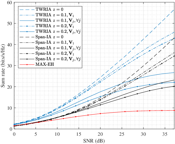
Figure 3 plots the sum rate versus SNR values for three types of precoders. First, it can be seen that the TWRIA algorithm provides better sum rates, which scales linearly with SNRs, as compared with the subspace alignment method (span-IA). Also, when the precoder is balanced for better energy harvesting, sum rates are decreased. When only single user employs balanced precoding, the sum rate is not reduced by a large amount, i.e., there is much less degree of freedom loss, as compared to the case when all users use the balanced precoding with the same CD value. Based on the required energy at the relay, the precoding can be balanced at users via different CD values. For a fixed CD value, the corresponding rate loss show an increase with SNR, as analyzed earlier in Lemma 5. Further, the decrements of sum rate with respect to the CD values can also be seen in the following rate-energy plots.
V-C Rate-energy plots
Given the precoders , the rate-energy region can be written as
| (34) |
For a splitting noise variance , the parametric plots are drawn to illustrate rate-energy regions [58, 59]. Figure 4 compares the same rate-energy region for different precoding schemes. The trend of different methods with various CD values is similar as in Figure 3. Different rates and energy plots conclude that energy harvesters can be improved at the expense of sum rate optimality.
Figure 5 shows the sum rate versus the harvested energy plot for aforementioned precoders with and without balanced precoding. It can be noted that the TWRIA region provides higher sum rates and lower energies, while the region for MAX-EH precoders has less sum rates and higher energies. These plots represent two extreme ends of rate and energy achievability. Next, for the balanced precoding, it can be observed that as increases, the rate decreases and the energy increases, when , where represents the threshold for CD. When , both rate and energy achieved are lower. Therefore, the value of CD () must be properly selected below the threshold to balance both the rates and the energy at each user.
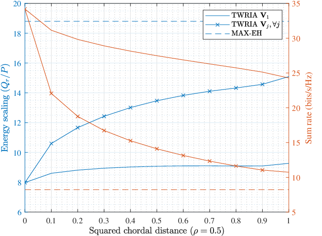
Figure 6 plots the sum rate (right-axis in red) and the harvested energy (left-axis in blue) versus the squared CD required for the balanced precoding with TWRIA and span-IA methods. It can be seen that the sum rate decreases in a logarithmic manner as increases. This behavior has been analyzed in the Lemma 5 for the rate-loss upper bound. On the other hand, the harvested energy increases if increases.
V-D QPSK symbol error rate versus SNR
Figure 7 depicts the average symbol error rate (SER) plots with uncoded QPSK modulation for . It can be seen that the perfect IA precoders () achieve the minimum SER, while with , the SER saturates. It can be noted the trend of error rate curves is same as in Figure 3, and the MAX-EH and the span-IA provide the worse SERs than that of TWRIA.
VI Conclusion
In this paper, for the TWR system, a modified IA algorithm is presented while considering AF relaying. To improve the SWIPT, i.e., to obtain the better rate-energy trade-offs, the CD decomposition-based balance precoding has been investigated, which is of low-complexity than the other SDR based convex relaxation-based suboptimal methods in the literature. Further, maximum energy based precoders, rate-loss upper bound, and harvested energy bounds are derived to show and compare the rate-energy trade-offs. Simulations with other IA methods conclude the effectiveness of the proposed IA and the CD decomposition-based balanced precoding schemes.
The future work is to investigate the effect of quantized or analog feedback including the specific details of 5G New Radio scenarios including imperfect CSI.
Appendices
-A IA Algorithm for TWR system
In the following, precoder and combiner expressions are derived to minimize the mean squared error (MSE), followed by an iterative procedure.
-A1 Receiver design
Given the precoders for , the receive combiner at the receiver can be obtained to minimize the MSE [43] as
The MSE at the user can be simplified as
Differentiating with respect to gives
yielding
| (35) |
where denotes the orthonormality operation as defined in the notations section.
-A2 Precoder design
Similarly, given the combiners , the transmit precoder can be optimized to minimize the total MSE as
The total MSE across all receivers can be rearranged as
Differentiating the above MSE with respect to provides
and simplifying to
| (36) |
where is added as a regularization term to avoid singular matrix for inverse. The value of regularizer parameter is chosen , that is close to the normalized noise power at the receiver .
-A3 Relay design (amplify-and-forward)
For an amplified and forward relay with , the factor can be obtained by solving the power constraint . Thus, we have
| (37) |
-A4 TWR-IA Algorithm
Combining the above procedure, an iterative procedure is given in Algorithm 2.
After initializing precoders, the scalar , decoders and precoders are iteratively updated until convergence. Since the scalar is changed every iteration, the effective channel is also updated per iteration. It can be seen via simulations that the number of iterations for convergence depends on SNR. The higher the SNR, the larger the number of iterations. Regarding the convergence, it can be seen that the above problem can be shown jointly convex with respect to as in [43]. Both steps minimize the same MSE, and the MSE is bounded to conclude the global convergence of the algorithm.
-B Proof of CD decomposition
-B1 Lemma 2
Consider two orthonormal matrices such that . Its left null space of size can be represented as . Then, we can write
| (38) |
where the last equation is obtained by the QR-decomposition such that and are and orthonormal matrices respectively. It verifies . Note that is independent of since is a projection to a lower dimension space. Also, the factors and are independent since represents the basis of and the basis is not unique. Using similar facts, the matrices and are also independent. For more details, visit [53]. The other two properties can be seen as follows. Consider the product simplifications for and as
and
-B2 Corollary 3
Let and be two set of precoders such that , i.e., from Lemma 2, with . The sum rate and the harvested energy will be the same, since the matrices with the zero CDs are related by a unitary matrix, which cannot change the value of the products , the products and the norm .
-B3 Corollary 4
From the CD decomposition, the desired displacement matrix can be computed as , where will be computed to satisfy the constraint in Lemma 2. The CD between this matrix and can be written as
where in , the singular value decomposition (SVD) of and with the same right singular vectors due to the constraint ; in , , are substituted, and the unitary matrix is multiplied into both arguments, since the resulting CD is unchanged for unitary multiplication, as in . This shows that and can be relaxed to a diagonal matrix.
-C Proof of Lemma 5: RLUB
Proof:
From the literature, we know that the rate loss is proportional to the interference [53, 60]. Therefore, the rate loss upper bound can be obtained as
where in (a), , and the inequality is obtained by Jensen’s inequality. Now, using the CD decomposition, one can write in terms of perfect IA precoder as
where using IA. In the above decomposition, and are independent of each other [53, Lemma 1]. The above matrix is not an orthonormal matrix. To make it orthonormal, let , subject to and , where via singular-value decomposition and , , and are independent of each other. Thus, the following product is composed of independent terms which can be simplified as
where in (a), the decomposition of has been substituted, and the expectation on is carried out, which is approximated to be as [53, App. B], with being the expected CD value; in (b), independence of basis matrices and is used; (c) is simplified from the fact that the product of two orthonormal matrices is matrix-Beta distributed random variable , which has a mean of . Next, we write for i.i.d. entries in and as
where in (a), ; in (b), the inequality is used (and verified via simulations); in (c), and are used; in (d), the fact that the norm of a vector is independent of its direction, and the approximation are used to get as
Finally, the rate loss bound expression can be simplified as
where . Substituting the value of provides the required expression. ∎
-D Proof of Lemma 7
Proof:
The inequality in the upper bound comes from (12a) as , where the inequality is due to the fact that the average of -values is less than the the maximum of them.
The inequality of the lower bound can be derived from the CD decomposition, where the equality occurs when . For the proposed balanced precoder with the optimum values of and , we can write
where in , the maximum value of the norm is upper bounded by trivial selection ; in , we employ the fact that the trace value in the expansion of norm is non-negative for the proposed scheme, as mentioned in the proposition 6; and in , the specific -dimensional null space can be replaced with any other -dimensional null space of . ∎
References
- [1] C. Yang, J. Li, Q. Ni, A. Anpalagan, and M. Guizani, “Interference-aware energy efficiency maximization in 5G ultra-dense networks,” IEEE Trans. Commun., vol. 65, no. 2, pp. 728–739, Dec. 2017.
- [2] J. L. Bing, Y. Rong, L. Gopal, and C. W. R. Chiong, “Transceiver design for SWIPT MIMO relay systems with hybridized power-time splitting-based relaying protocol,” IEEE Access, vol. 8, pp. 190 922–190 933, 2020.
- [3] H. Mahmoud Gamal ElDin Mohammed ElAnzeery, Mohamed Abd ElAziz Saad ElBagouri, and R. Guindi, “Novel radio frequency energy harvesting model,” in Proc. IEEE International Power Engineering and Optimization Conference, Melaka, Malaysia, June 2012.
- [4] R. J. Vyas, B. B. Cook, Y. Kawahara, and M. M. Tentzeris, “E-WEHP: A batteryless embedded sensor-platform wirelessly powered from ambient digital-TV signals,” IEEE Trans. Microw. Theory Techn., vol. 61, no. 6, pp. 2491–2505, May 2013.
- [5] I. Krikidis, S. Timotheou, S. Nikolaou, G. Zheng, D. W. K. Ng, and R. Schober, “Simultaneous wireless information and power transfer in modern communication systems,” IEEE Commun. Mag., vol. 52, no. 11, pp. 104–110, Nov. 2014.
- [6] C. Valenta and G. Durgin, “Harvesting wireless power: Survey of energy-harvester conversion efficiency in far-field, wireless power transfer systems,” IEEE Microwave Magazine, vol. 15, no. 4, pp. 108–120, 2014.
- [7] H. Shen, C. Liu, W. Xu, and C. Zhao, “Optimized full-duplex MIMO DF relaying with limited dynamic range,” IEEE Access, vol. 5, pp. 20 726–20 735, Sep. 2017.
- [8] O. Taghizadeh, A. C. Cirik, and R. Mathar, “Hardware impairments aware transceiver design for full-duplex amplify-and-forward MIMO relaying,” IEEE Trans. Wireless Commun., vol. 17, no. 3, pp. 1644–1659, Dec. 2018.
- [9] Z. Wen, X. Liu, N. C. Beaulieu, R. Wang, and S. Wang, “Joint source and relay beamforming design for full-duplex MIMO af relay SWIPT systems,” IEEE Communications Letters, vol. 20, no. 2, pp. 320–323, 2016.
- [10] D. Wang, R. Zhang, X. Cheng, and L. Yang, “Capacity-enhancing full-duplex relay networks based on power-splitting (PS-)SWIPT,” IEEE Transactions on Vehicular Technology, vol. 66, no. 6, pp. 5445–5450, 2017.
- [11] W. Wang, R. Wang, W. Duan, R. Feng, and G. Zhang, “Optimal transceiver designs for wireless-powered full-duplex two-way relay networks with SWIPT,” IEEE Access, vol. 5, pp. 22 329–22 343, 2017.
- [12] L. Bariah, S. Muhaidat, and A. Al-Dweik, “Error probability analysis of noma-based relay networks with SWIPT,” IEEE Communications Letters, vol. 23, no. 7, pp. 1223–1226, 2019.
- [13] X. Sun, W. Yang, Y. Cai, Z. Xiang, and X. Tang, “Secure transmissions in millimeter wave swipt uav-based relay networks,” IEEE Wireless Communications Letters, vol. 8, no. 3, pp. 785–788, 2019.
- [14] X. Wang, J. Liu, and C. Zhai, “Wireless power transfer-based multi-pair two-way relaying with massive antennas,” IEEE Transactions on Wireless Communications, vol. 16, no. 11, pp. 7672–7684, 2017.
- [15] S. Gautam, T. X. Vu, S. Chatzinotas, and B. Ottersten, “Cache-aided simultaneous wireless information and power transfer (SWIPT) with relay selection,” IEEE Journal on Selected Areas in Communications, vol. 37, no. 1, pp. 187–201, 2019.
- [16] Y. Hu, Y. Zhu, M. C. Gursoy, and A. Schmeink, “SWIPT-enabled relaying in iot networks operating with finite blocklength codes,” IEEE Journal on Selected Areas in Communications, vol. 37, no. 1, pp. 74–88, 2019.
- [17] J. Yan and Y. Liu, “A dynamic SWIPT approach for cooperative cognitive radio networks,” IEEE Transactions on Vehicular Technology, vol. 66, no. 12, pp. 11 122–11 136, 2017.
- [18] X. Chen, D. W. K. Ng, and H. Chen, “Secrecy wireless information and power transfer: challenges and opportunities,” IEEE Wireless Communications, vol. 23, no. 2, pp. 54–61, 2016.
- [19] X. Lu, P. Wang, D. Niyato, D. I. Kim, and Z. Han, “Wireless networks with RF energy harvesting: A contemporary survey,” IEEE Communications Surveys Tutorials, vol. 17, no. 2, pp. 757–789, 2015.
- [20] M. A. Hossain, R. Md Noor, K. A. Yau, I. Ahmedy, and S. S. Anjum, “A survey on simultaneous wireless information and power transfer with cooperative relay and future challenges,” IEEE Access, vol. 7, pp. 19 166–19 198, 2019.
- [21] D. K. P. Asiedu, H. Lee, and K. Lee, “Simultaneous wireless information and power transfer for decode-and-forward multihop relay systems in energy-constrained IoT networks,” IEEE Internet of Things Journal, vol. 6, no. 6, pp. 9413–9426, 2019.
- [22] R. Fan, S. Atapattu, W. Chen, Y. Zhang, and J. Evans, “Throughput maximization for multi-hop decode-and-forward relay network with wireless energy harvesting,” IEEE Access, vol. 6, pp. 24 582–24 595, 2018.
- [23] G. Huang, Q. Zhang, and J. Qin, “Joint time switching and power allocation for multicarrier decode-and-forward relay networks with SWIPT,” IEEE Signal Processing Letters, vol. 22, no. 12, pp. 2284–2288, 2015.
- [24] B. Chen, X. Zhu, and X. Tu, “Joint precoder design for SWIPT-enabled MIMO relay networks with finite-alphabet inputs,” IEEE Access, vol. 8, pp. 179 105–179 117, 2020.
- [25] B. Chen, X. Zhu, X. Tu, and Y. Guo, “Linear precoder design for SWIPT-enabled relay networks with finite-alphabet inputs,” IEEE Access, vol. 8, pp. 82 012–82 023, 2020.
- [26] Z. Wen, X. Liu, S. Zheng, and W. Guo, “Joint source and relay design for mimo two-way relay networks with SWIPT,” IEEE Transactions on Vehicular Technology, vol. 67, no. 1, pp. 822–826, 2018.
- [27] X. Zhou and Q. Li, “Energy efficiency optimisation for SWIPT af two-way relay networks,” Electronics Letters, vol. 53, no. 6, pp. 436–438, 2017.
- [28] ——, “Energy efficiency for SWIPT in MIMO two-way amplify-and-forward relay networks,” IEEE Transactions on Vehicular Technology, vol. 67, no. 6, pp. 4910–4924, 2018.
- [29] J. Rostampoor, S. M. Razavizadeh, and I. Lee, “Energy efficient precoding design for SWIPT in MIMO two-way relay networks,” IEEE Transactions on Vehicular Technology, vol. 66, no. 9, pp. 7888–7896, 2017.
- [30] H. K. Sahu and P. R. Sahu, “SSK-based SWIPT with AF relay,” IEEE Communications Letters, vol. 23, no. 4, pp. 756–759, 2019.
- [31] H. Lee, C. Song, S. Choi, and I. Lee, “Outage probability analysis and power splitter designs for SWIPT relaying systems with direct link,” IEEE Communications Letters, vol. 21, no. 3, pp. 648–651, 2017.
- [32] Y. Ye, Y. Li, D. Wang, F. Zhou, R. Q. Hu, and H. Zhang, “Optimal transmission schemes for DF relaying networks using SWIPT,” IEEE Transactions on Vehicular Technology, vol. 67, no. 8, pp. 7062–7072, 2018.
- [33] Y. Ye, Y. Li, Z. Wang, X. Chu, and H. Zhang, “Dynamic asymmetric power splitting scheme for SWIPT-based two-way multiplicative AF relaying,” IEEE Signal Processing Letters, vol. 25, no. 7, pp. 1014–1018, 2018.
- [34] H. Chen, Y. Li, Y. Jiang, Y. Ma, and B. Vucetic, “Distributed power splitting for SWIPT in relay interference channels using game theory,” IEEE Transactions on Wireless Communications, vol. 14, no. 1, pp. 410–420, 2015.
- [35] G. Li, D. Mishra, Y. Hu, and S. Atapattu, “Optimal designs for relay-assisted NOMA networks with hybrid SWIPT scheme,” IEEE Transactions on Communications, vol. 68, no. 6, pp. 3588–3601, 2020.
- [36] W. Wang, R. Wang, H. Mehrpouyan, N. Zhao, and G. Zhang, “Beamforming for simultaneous wireless information and power transfer in two-way relay channels,” IEEE Access, vol. 5, pp. 9235–9250, 2017.
- [37] Y. Cai, M. Zhao, Q. Shi, B. Champagne, and M. Zhao, “Joint transceiver design algorithms for multiuser MISO relay systems with energy harvesting,” IEEE Transactions on Communications, vol. 64, no. 10, pp. 4147–4164, 2016.
- [38] H. Du, T. Ratnarajah, M. Sellathurai, and C. B. Papadias, “Reweighted nuclear norm approach for interference alignment,” IEEE Transactions on Communications, vol. 61, no. 9, pp. 3754–3765, 2013.
- [39] S. M. Razavi and T. Ratnarajah, “Performance analysis of interference alignment under csi mismatch,” IEEE Transactions on Vehicular Technology, vol. 63, no. 9, pp. 4740–4748, 2014.
- [40] Y. Luo, T. Ratnarajah, J. Xue, and F. A. Khan, “Interference alignment in two-tier randomly distributed heterogeneous wireless networks using stochastic geometry approach,” IEEE Systems Journal, vol. 12, no. 3, pp. 2238–2249, 2018.
- [41] J. Xue, S. Biswas, A. C. Cirik, H. Du, Y. Yang, T. Ratnarajah, and M. Sellathurai, “Transceiver design of optimum wirelessly powered full-duplex mimo iot devices,” IEEE Transactions on Communications, vol. 66, no. 5, pp. 1955–1969, 2018.
- [42] V. Cadambe and S. Jafar, “Interference alignment and degrees of freedom of the K-user interference channel,” IEEE Transactions on Information Theory, vol. 54, no. 8, pp. 3425–3441, 2008.
- [43] N. Garg, A. K. Jagannatham, G. Sharma, and T. Ratnarajah, “Precoder feedback schemes for robust interference alignment with bounded CSI uncertainty,” IEEE Transactions on Signal and Information Processing over Networks, vol. 6, pp. 407–425, 2020.
- [44] Z. Xie, X. Geng, Y. Chen, K. Song, B. Panful, Y. Wang, Y. Su, Z. Zhang, and Y. Hu, “Secured green communication scheme for interference alignment based networks,” Journal of Communications and Networks, vol. 22, no. 1, pp. 23–36, 2020.
- [45] M. Chu, B. He, X. Liao, Z. Gao, and V. C. M. Leung, “On the design of power splitting relays with interference alignment,” IEEE Transactions on Communications, vol. 66, no. 4, pp. 1411–1424, 2018.
- [46] F. Benkhelifa, A. S. Salem, and M. Alouini, “Sum-rate enhancement in multiuser MIMO decode-and-forward relay broadcasting channel with energy harvesting relays,” IEEE Journal on Selected Areas in Communications, vol. 34, no. 12, pp. 3675–3684, 2016.
- [47] Z. Fang, Y. Wu, Y. Lu, J. Hu, T. Peng, and J. Ye, “Simultaneous wireless information and power transfer in cellular two-way relay networks with massive MIMO,” IEEE Access, vol. 6, pp. 29 262–29 270, 2018.
- [48] R. S. Ganesan, T. Weber, and A. Klein, “Interference alignment in multi-user two way relay networks,” in Proc. IEEE 73rd Vehicular Technology Conference (VTC Spring), Yokohama, Japan, May 2011.
- [49] L. Shi, Y. Ye, R. Q. Hu, and H. Zhang, “Energy efficiency maximization for SWIPT enabled two-way DF relaying,” IEEE Signal Processing Letters, vol. 26, no. 5, pp. 755–759, 2019.
- [50] J. Wang, G. Wang, B. Li, H. Yang, Y. Hu, and A. Schmeink, “Massive MIMO two-way relaying systems with SWIPT in IoT networks,” IEEE Internet of Things Journal, pp. 1–14, Oct. 2020.
- [51] Z. Zong, H. Feng, F. R. Yu, N. Zhao, T. Yang, and B. Hu, “Optimal transceiver design for SWIPT in K-user MIMO interference channels,” IEEE Trans. Wireless Commun., vol. 15, no. 1, pp. 430–445, Aug. 2016.
- [52] C. M. Yetis, T. Gou, S. A. Jafar, and A. H. Kayran, “On feasibility of interference alignment in MIMO interference networks,” IEEE Trans. Signal Process., vol. 58, no. 9, pp. 4771–4782, May 2010.
- [53] N. Ravindran and N. Jindal, “Limited feedback-based block diagonalization for the MIMO broadcast channel,” IEEE J. Sel. Areas Commun., vol. 26, no. 8, pp. 1473–1482, Oct. 2008.
- [54] N. Garg and G. Sharma, “Analog precoder feedback schemes with interference alignment,” IEEE Transactions on Wireless Communications, vol. 17, no. 8, pp. 5382–5396, Aug 2018.
- [55] N. Zhao, F. Yu, and V. Leung, “Wireless energy harvesting in interference alignment networks,” IEEE Communications Magazine, vol. 53, no. 6, pp. 72–78, 2015.
- [56] Y. Li, L. Zhang, L. J. Cimini, and H. Zhang, “Statistical analysis of MIMO beamforming with co-channel unequal-power MIMO interferers under path-loss and rayleigh fading,” IEEE Transactions on Signal Processing, vol. 59, no. 8, pp. 3738–3748, 2011.
- [57] R. S. Ganesan, H. Al-Shatri, A. Kuehne, T. Weber, and A. Klein, “Pair-aware interference alignment in multi-user two-way relay networks,” IEEE Trans. Wireless Commun., vol. 12, no. 8, pp. 3662–3671, May 2013.
- [58] X. Zhou, R. Zhang, and C. Ho, “Wireless information and power transfer: Architecture design and rate-energy tradeoff,” IEEE Transactions on Communications, vol. 61, no. 11, pp. 4754–4767, 2013.
- [59] J. Kang, I. Kim, and D. I. Kim, “Wireless information and power transfer: Rate-energy tradeoff for nonlinear energy harvesting,” IEEE Transactions on Wireless Communications, vol. 17, no. 3, pp. 1966–1981, 2018.
- [60] O. E. Ayach and R. W. Heath, “Interference alignment with analog channel state feedback,” IEEE Trans. Wireless Commun., vol. 11, no. 2, pp. 626–636, Dec. 2012.