Projection based model reduction for the immersed boundary method

The IBM is intended for the computer simulation of FSI, especially in biological fluid dynamics. It is mathematically defined by a set of differential equations involving a mixture of Eulerian and Lagrangian descriptions, linked by the Dirac delta function. The dynamics of the fluid is described in terms of the velocity $\boldsymbol{u}(\boldsymbol{x},t)$ and the pressure $p(\boldsymbol{x},t)$ on an Eulerian coordinate for $\boldsymbol{x}\in\Omega$, where $\Omega\subset\mathbb{R}^{d},\ d=2\text{ or }3$, represents the fluid domain. The immersed structures, on the other hand, are handled in a Lagrangian coordinate as a parametric curve or surface $X(\boldsymbol{s},t)$. Specifically, $X(\boldsymbol{s},t)$ represents the position at time $t$ in Cartesian coordinates of the structure point labeled by $\boldsymbol{s}\in\Gamma$, where $\Gamma\subset\mathbb{R}^{d-1}$ is the parameter space. In this work, we focus on two-dimensional flows where the structure is described as a parametric curve. In this case $\boldsymbol{x}\in\Omega\subset\mathbb{R}^{2}$ and $s$ is a scalar parameter. The formulation is mostly algebraic. Therefore the extension to high dimensional cases is straightforward. Assuming constant density, the time-dependent Stokes equation is used to model the incompressible flow

where $\rho$ and $\mu$ are the fluid density and viscosity, respectively. The body force $\boldsymbol{f}$ exerted by the structure on the fluid is defined as

where $\delta(\boldsymbol{x})$ is the Dirac delta function. In addition, $\boldsymbol{F}(s,t)$ denotes the force density on the immersed structure, defined as

where $\boldsymbol{\mathcal{F}}$ is a functional of the IBM configuration. Spring forces, bending resistance or any other type of behavior (area and volume conservation constraints) can be built into this functional to embody the physics of the immersed structure under different circumstances [19, 33]. We give detailed description of the force density in section 4 in the numerical examples for various systems.

Assuming an over-damped structure, the immersed boundary must move with the local fluid velocity:

This last equation is nothing other than the no-slip condition written as a delta function convolution.

To derive a semi-discrete representation of the IBM, we use the finite difference discretization [13]. Other numerical methods can also be applied to discretize the IBM, e.g., the finite element method [34] and the finite volume method [35], in which the state space consists of nodal values.

In this work, fluid variables are discretized on a uniform staggered Eulerian grid, denoted $\Omega_{h}$; and the structures are discretized on an independent Lagrangian grid, denoted by $\Gamma_{h}$ (Fig 1). The Eulerian grid points are of the form $\boldsymbol{x}=\boldsymbol{j}h$, where $\boldsymbol{j}=(j_{1},j_{2})$ is a two-dimensional vector with integer components and $h$ is the Eulerian grid size. The Lagrangian grid is a set of $s$ of the form $k\Delta s$, where $k$ has integer components. The following restriction is imposed to avoid leak[13],

for all $s$.

First, the semi-discrete equations for (1)-(2) form a system of linear differential-algebraic equations (DAEs)

where

are vectors of discrete velocity field, pressure and body force, respectively. $G\in\mathbb{R}^{n_{u},n_{u}}$ is the discrete Laplace operator. Matrices $N\in\mathbb{R}^{n_{u},n_{p}}$ and $M\in\mathbb{R}^{n_{p},n_{u}}$ are the discrete gradient and divergence operators, respectively.

Second, the integrals in (3) and (5) are replaced by the following sums over the appropriate grid points,

where $F_{h}(s,t)$ is the discrete Lagrangian force density associated with the structure point labeled $s$, obtained by discretizing (4). In addition, a function $\delta_{r}(\boldsymbol{x})$ that is nonsingular for each $r$ but approaches $\delta(\boldsymbol{x})$ as $r\to 0$ is needed. There are many ways to construct such $\delta_{r}$. We choose a radially symmetric function with compact support as follows [36],

where the normalizing constant $C_{r}=\frac{10}{3\pi}r^{-2}$ depends on $r$ and the space dimension ($C_{r}=\frac{15}{4\pi}r^{-3}$ in 3D). For computational efficiency, we choose $r=2h$ in all our numerical experiments, as suggested for IBM [13].

Meanwhile, equations (9) and (10) can be put into matrix-vector form:

where

are the discrete representations of the structure position and the Lagrangian force density. Using natural arrangement of the fluid variables, $B\in\mathbb{R}^{n_{u},n_{s}}$ can be constructed as a block matrix

A column of each $B_{k}$ consists of evaluations of $\delta_{r}(\boldsymbol{x}-X(s,t))$ for a fixed $X(s,t)$ on grid points $\boldsymbol{x}$ that store one component of the fluid velocity variables. For example, the $i,j$-entry of $B_{1}$ is $\delta_{r}(\boldsymbol{x}_{i}-X(s_{j},t))$, where $\boldsymbol{x}_{i}$ is the grid point that stores the $i$th fluid velocity in the $x$-direction. Note that $B_{k}$’s are not identical because they correspond to different Eulerian grid points $\boldsymbol{x}$. For example in Fig 1, $\boldsymbol{x}$ in $B_{1}$ are the points marked by filled triangles, while $\boldsymbol{x}$ in $B_{2}$ are marked by stars. We also point out that $B$ is time dependent due to its dependence on $\boldsymbol{X}_{h}(t)$.

Lastly, by substituting (12) into (7) for $\boldsymbol{f}_{h}(t)$, we get the following DAE system which we shall refer to as the FOM

In general, the number of structure variables is much less than the number of fluid variables, i.e., $n_{s}\ll n_{u}$. In fact, $\delta_{r}$ having compact support means only a small fraction of the Eulerian grid points are directly interacting with the structure. If one is only interested in the motion of the structure, i.e. $\boldsymbol{X}_{h}(t)$, solving the system (15)-(17) becomes a reduced-order problem [37], where $\boldsymbol{F}_{h}(t)$ is the low-dimensional input and $\dot{\boldsymbol{X}}_{h}(t)$ is the low-dimensional output.

We propose the following choice of $V$ and $W$,

For later reference, note that both subspaces vary in time. The resulting coefficient matrices are given by

In principle, one can use higher dimensional Krylov subspaces ($V$ and $W$ with more columns), followed by Lanczos orthogonalization algorithms [26, 37, 38], to improve the accuracy of the ROM. Specifically, we shall see in the following discussion that our choice satisfies two interpolation conditions. Higher dimensional Krylov subspaces are able to interpolate the transfer function more accurately by enforcing more interpolation conditions, but at the expense of a reduced computational speedup. From the numerical tests, our observation is that the current subspaces achieve a good balance between accuracy and efficiency.

Because the coefficient matrices in the ROM are in principle time dependent, they should be updated frequently during simulation. Direct matrix multiplication for this purpose is time consuming since $Q$ is a dense matrix in $\mathbb{R}^{2n_{u},2n_{u}}$. For example, computing $M_{1}$ in (35) has complexity $O(n_{u}^{2})$. In the rest of this section, we propose a computationally cheaper approach using interpolation to approximate the coefficients.

We first approximate $\dot{B}$ by

One could consider a higher order discretizations for $\dot{B}$ so that a method of order higher than one in time can be used to solve the ROM. Ultimately, this is a trade-off between accuracy and the offline interpolation efficiency. From the numerical tests, we will see such first order approximation of $\dot{B}$ together with the forward Euler’s method provides acceptable accuracy for the numerical tests compared to the FOM.

The other observation is that the matrix $M_{1}$ is then approximated by

Together with $M_{0}=B(t)^{T}QB(t)$, the following three matrices are needed for building our ROM

Since $Q$ and $G$ are constant matrices, the $i,j$-entry of any of the above matrices at time $t$ is determined by the $i$th row of $B(t)^{T}$ and the $j$th column of $B(t)$ (or $B(t-\Delta t)$). Recall that each column of $B(t)$ (or row of $B(t)^{T}$) represents a smoothed delta function associated with a structure point. Suppose the $i$th column of $B(t)^{T}$ is associated with the Lagrangian grid point $X_{l}\in\mathbb{R}^{d}$ ($d=2,3$) and the $j$th column of $B(t)^{T}$ (or $B(t-dt)$) is associated with $X_{r}\in\mathbb{R}^{d}$. Given the prescribed function $\delta_{r}$ and a fixed Eulerian grid, the $i,j$-entry of a coefficient matrix is uniquely determined by $X_{l}$ and $X_{r}$, which can be viewed as a function from $\mathbb{R}^{2d}$ to $\mathbb{R}$. It is then natural to sample such functions before the simulation starts. As the simulation runs, coefficient matrices are updated by interpolation using precomputed samples. In this work, linear interpolation is used. Because each entry of the $2n_{s}$-by-$2n_{s}$ coefficient matrix is obtained by evaluating a precomputed linear function, the complexity is typically $O(n_{s}^{2})$, which is much smaller than the complexity of direct matrix multiplications $O(n_{u}^{2})$, given $n_{s}\ll n_{u}$.

Next, motivated by our numerical experiments illustrated in Fig 2, we show that the interpolated $2d$-dimensional functions of $X_{l}$ and $X_{r}$ can be well approximated by $d$-dimensional functions of $X_{l}-X_{r}$, i.e., the relative position of the two points. Such low-dimensional approximation significantly reduces the number of samples needed for more accurate interpolations. Hence the sampling process can also be accelerated.

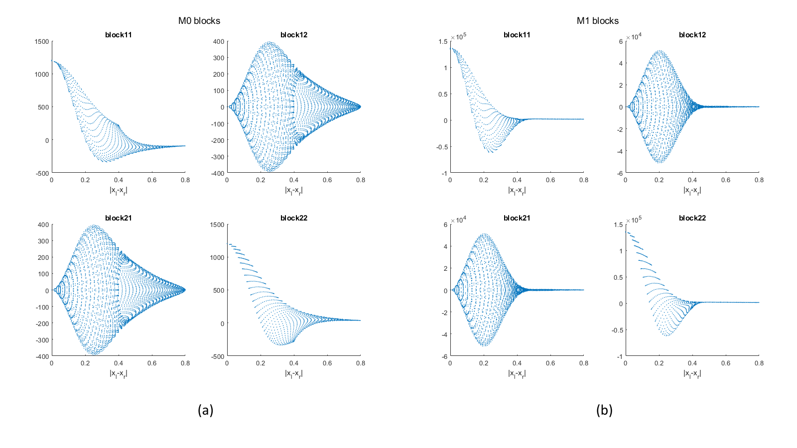
Here we provide justifications of this approach by making connections to the Green’s functions. Recall that $Q=I-N(MN)^{-1}M$, where $N$ and $M$ are discrete gradient and divergence operators. Therefore, each entry of the matrix $B(t)^{T}QB(t)$ or $B(t)^{T}QB(t-\Delta t)$ is a numerical approximation of the integral

where $i,j=1,\cdots,d$ and $d=2$ or $3$. $\delta_{ij}$ is the Kronecker delta function. $I_{1}$ only depends on $|X_{l}-X_{r}|$ due to our choice of $\delta_{r}$. For $I_{2}$, we assume $X_{l}$ and $X_{r}$ are far from the boundary of $\Omega$ so the Green’s function $G(\boldsymbol{x},\boldsymbol{y})$ can be applied. Considering the limiting case of $r\to 0$, i.e., $\delta_{r}\to\delta$, as $r\to 0,$ and we arrive at,

which depends only on $X_{l}-X_{r}$.

Similarly, each entry of the matrix $B(t)^{T}QGQB(t)$ is a numerical approximation of the following integral

where $J_{11}$ and $J_{21}$ depend on $X_{l}-X_{r}$ due to our choice of $\delta_{r}$. For $J_{12}$ and $J_{22}$ we make the same assumptions as for $I_{2}$ and consider the limiting case. We obtain similar results

So both terms depend only on $X_{l}-X_{r}$. However, the integrals $I_{0}$ and $J_{0}$ may not be further reduced to functions of $|X_{l}-X_{r}|$, as suggested by our numerical experiments, see Fig 3.

We consider the oscillations of a pressurized fiber. Initially, the stretched elastic fiber resides in the center of a resting fluid. The semi-major and semi-minor axes of the fiber are 0.4 and 0.2 $\mu m$, respectively. The fluid domain is $4\mu m\times 4\mu m$ with periodic boundary conditions on all edges. Fluid density and viscosity are chosen so that the Reynolds number is $0.01$. The body force in this example is generated by an elastic energy functional [13],

where $\varepsilon$ is the local energy given by

which corresponds to an elastic fiber having a ”spring constant” $\sigma$ and an equilibrium state where the elastic strain $|\partial\boldsymbol{X}/\partial s|\equiv L$. The force in (4) is then expressed as

References

- [1] Clement Kleinstreuer. Biofluid Dynamics: Principles and Selected Applications. CRC Press, 2006.
- [2] S. Canic. Blood flow through compliant vessels after endovascular repair: wall deformations induced by the discontinuous wall properties. Computing and Visualization in Science, 4(3):147–155, 2002.
- [3] S. Canic and D. Mirkovic. A hyperbolic system of conservation laws in modeling endovascular treatment of abdominal aortic aneurysm. In Heinrich Freistühler and Gerald Warnecke, editors, Hyperbolic Problems: Theory, Numerics, Applications, volume 140, pages 227–236. Birkhäuser Basel, Basel, 2001.
- [4] Huan Lei and George Em Karniadakis. Predicting the morphology of sickle red blood cells using coarse-grained models of intracellular aligned hemoglobin polymers. Soft Matter, 8(16):4507–4516, 2012.
- [5] Xuejin Li, Zhangli Peng, Huan Lei, Ming Dao, and George Em Karniadakis. Probing red blood cell mechanics, rheology and dynamics with a two-component multi-scale model. Philosophical Transactions of the Royal Society A: Mathematical, Physical and Engineering Sciences, 372(2021):20130389, 2014.
- [6] Q. Wang. A hydrodynamic theory for solutions of nonhomogeneous nematic liquid crystalline polymers of different configurations. The Journal of Chemical Physics, 116(20):9120–9136, 2002.
- [7] X. Yang, G. Forest, W. Mullins, and Q. Wang. Dynamic defect morphology and hydrodynamics of sheared nematic polymers in two space dimensions. Journal of Rheology, 53(3):589–615, 2009.
- [8] Yue Yu. Fluid-structure interaction modeling in 3d cerebral arteries and aneurysms. In Peter Wriggers and Thomas Lenarz, editors, Biomedical Technology: Modeling, Experiments and Simulation, pages 123–146. Springer, Cham, 2018.
- [9] J. Zhao, X. Yang, J. Shen, and Q. Wang. A decoupled energy stable scheme for a hydrodynamic phase-field model of mixtures of nematic liquid crystals and viscous fluids. Journal of Computational Physics, 305:539–556, 2016.
- [10] William S Hall. The Boundary Element Method, volume 27. Springer Netherlands, 1 edition, 1994.
- [11] Shuwang Li and Xiaofan Li. A boundary integral method for computing the dynamics of an epitaxial island. SIAM Journal on Scientific Computing, 33(6):3282–3302, 2011.
- [12] Gordon C Everstine and Francis M Henderson. Coupled finite element/boundary element approach for fluid–structure interaction. The Journal of the Acoustical Society of America, 87(5):1938–1947, 1990.
- [13] Charles S Peskin. The immersed boundary method. Acta numerica, 11:479–517, 2002.
- [14] Ming-Chih Lai and Charles S Peskin. An immersed boundary method with formal second-order accuracy and reduced numerical viscosity. Journal of Computational Physics, 160(2):705–719, 2000.
- [15] Paul J. Atzberger, Peter R. Kramer, and Charles S. Peskin. A stochastic immersed boundary method for fluid-structure dynamics at microscopic length scales. Journal of Computational Physics, 224(2):1255–1292, June 2007.
- [16] Fotis Sotiropoulos and Xiaolei Yang. Immersed boundary methods for simulating fluid–structure interaction. Progress in Aerospace Sciences, 65:1–21, 2014.
- [17] Randall J Leveque and Zhilin Li. The immersed interface method for elliptic equations with discontinuous coefficients and singular sources. SIAM Journal on Numerical Analysis, 31(4):1019–1044, 1994.
- [18] Roland Glowinski, Tsorng-Whay Pan, and Jacques Periaux. A fictitious domain method for dirichlet problem and applications. Computer Methods in Applied Mechanics and Engineering, 111(3-4):283–303, 1994.
- [19] Wenrui Hao, Zhiliang Xu, Chun Liu, and Guang Lin. A fictitious domain method with a hybrid cell model for simulating motion of cells in fluid flow. Journal of Computational Physics, 280:345–362, 2015.
- [20] Grétar Tryggvason, Bernard Bunner, Asghar Esmaeeli, Damir Juric, N Al-Rawahi, W Tauber, J Han, S Nas, and Y-J Jan. A front-tracking method for the computations of multiphase flow. Journal of Computational Physics, 169(2):708–759, 2001.
- [21] James Glimm, Xiaolin Li, Yingjie Liu, Zhiliang Xu, and Ning Zhao. Conservative front tracking with improved accuracy. SIAM Journal on Numerical Analysis, 41(5):1926–1947, 2003.
- [22] Georges-Henri Cottet and Emmanuel Maitre. A level set method for fluid-structure interactions with immersed surfaces. Mathematical models and methods in applied sciences, 16(03):415–438, 2006.
- [23] Qiang Du, Chun Liu, and Xiaoqiang Wang. A phase field approach in the numerical study of the elastic bending energy for vesicle membranes. Journal of Computational Physics, 198(2):450–468, 2004.
- [24] Catherine Kublik, Nicolay M Tanushev, and Richard Tsai. An implicit interface boundary integral method for poisson’s equation on arbitrary domains. Journal of Computational Physics, 247:279–311, 2013.
- [25] Ivo Babuska and J. Tinsley Oden. Verification and validation in computational engineering and science: basic concepts. Computer Methods in Applied Mechanics and Engineering, 193:4057–4066, 2004.
- [26] Zhaojun Bai. Krylov subspace techniques for reduced-order modeling of large-scale dynamical systems. Applied Numerical Mathematics, 43(1-2):9–44, Apr 2002.
- [27] Peter Benner, Serkan Gugercin, and Karen Willcox. A survey of projection-based model reduction methods for parametric dynamical systems. SIAM Review, 57(4):483–531, 2015.
- [28] S. Gugercin, A. Antoulas, and C. Beattie. Model Reduction for Large-Scale Linear Dynamical Systems. SIAM Journal on Matrix Analysis and Applications, 30(2):609–638, 2008.
- [29] Branimir Anic. An interpolation-based approach to the weighted model reduction problem. PhD thesis, Virginia Polytechnic Institute and State University, Virginia, 2008.
- [30] Yuanxun Bao, Aleksandar Donev, Boyce E Griffith, David M McQueen, and Charles S Peskin. An immersed boundary method with divergence-free velocity interpolation and force spreading. Journal of Computational Physics, 347:183–206, 2017.
- [31] Alessandro Nitti, Josef Kiendl, Alessandro Reali, and Marco D de Tullio. An immersed-boundary/isogeometric method for fluid–structure interaction involving thin shells. Computer Methods in Applied Mechanics and Engineering, 364:112977, 2020.
- [32] Anvar Gilmanov, Trung Bao Le, and Fotis Sotiropoulos. A numerical approach for simulating fluid structure interaction of flexible thin shells undergoing arbitrarily large deformations in complex domains. Journal of Computational Physics, 300:814–843, 2015.
- [33] Igor V Pivkin and George Em Karniadakis. Accurate coarse-grained modeling of red blood cells. Physical Review Letters, 101(11):118105, 2008.
- [34] Daniele Boffi and Lucia Gastaldi. A finite element approach for the immersed boundary method. Computers & Structures, 81(8-11):491–501, 2003.
- [35] Jungwoo Kim, Dongjoo Kim, and Haecheon Choi. An immersed-boundary finite-volume method for simulations of flow in complex geometries. Journal of Computational Physics, 171(1):132–150, 2001.
- [36] Jerry Zhijian Yang, Xiaojie Wu, and Xiantao Li. A generalized irving–kirkwood formula for the calculation of stress in molecular dynamics models. The Journal of Chemical Physics, 137(13):134104, 2012.
- [37] Roland W Freund. Krylov-subspace methods for reduced-order modeling in circuit simulation. Journal of Computational and Applied Mathematics, 123(1-2):395–421, 2000.
- [38] Lina Ma, Xiantao Li, and Chun Liu. Coarse-graining langevin dynamics using reduced-order techniques. Journal of Computational Physics, 380:170–190, 2019.
- [39] George Barker Jeffery. The motion of ellipsoidal particles immersed in a viscous fluid. Proceedings of the Royal Society of London. Series A, 102(715):161–179, 1922.
- [40] Julie Behr, Byron Gaskin, Changliang Fu, Cheng Dong, and Robert Kunz. Localized modeling of biochemical and flow interactions during cancer cell adhesion. PloS One, 10(9):e0136926, 2015.
- [41] A. Coclite, S. Ranaldo, M.D. de Tullio, P. Decuzzi, and G. Pascazio. Kinematic and dynamic forcing strategies for predicting the transport of inertial capsules via a combined lattice boltzmann – immersed boundary method. Computers and Fluids, 180:41–53, 2019.