Stagnation Detection with
Randomized Local Search
Abstract
Recently a mechanism called stagnation detection was proposed that automatically adjusts the mutation rate of evolutionary algorithms when they encounter local optima. The so-called SD-(1+1) EA introduced by Rajabi and Witt (GECCO 2020) adds stagnation detection to the classical (1+1) EA with standard bit mutation, which flips each bit independently with some mutation rate, and raises the mutation rate when the algorithm is likely to have encountered local optima.
In this paper, we investigate stagnation detection in the context of the -bit flip operator of randomized local search that flips bits chosen uniformly at random and let stagnation detection adjust the parameter . We obtain improved runtime results compared to the SD-(1+1) EA amounting to a speed-up of up to Moreover, we propose additional schemes that prevent infinite optimization times even if the algorithm misses a working choice of due to unlucky events. Finally, we present an example where standard bit mutation still outperforms the local -bit flip with stagnation detection.
1 Introduction
Evolutionary Algorithms (EAs) are parameterized algorithms, so it has been ongoing research to discover how to choose their parameters best. Static parameter settings are not efficient for a wide range of problems. Also, given a specific problem, there might be different scenarios during the optimization, which results in inefficiency of one static parameter configuration for the whole run. Self-adjusting mechanisms address this issue as a non-static parameter control framework that can learn acceptable or even near-optimal parameter settings on the fly. See also the survey article Doerr and Doerr 2020 for a detailed coverage of static and non-static parameter control.
Many studies have been conducted on frameworks which adjust the mutation rate of different mutation operators, in particular in the standard bit mutation for the search space of bit strings to make the rate efficient on unimodal functions. For example, the ) GA using the -rule can adjust its mutation strength (and also its crossover rate) on OneMax (Doerr and Doerr 2018), resulting in asymptotic speed-ups compared to static settings. Likewise, the self-adjusting mechanism in the (1+) EA with two rates proposed in Doerr et al. 2019 performs on unimodal functions as efficiently as the best -parallel unary unbiased black-box algorithm.
The self-adjusting frameworks mentioned above are mainly designed to optimize unimodal functions. Generally, they are not able to suggest an efficient parameter setting where algorithms get stuck in a local optimum since they mainly work based on the number of successes, so there is no signal in such a situation. On multimodal functions, where some specific numbers of bits have to flip to make progress, Stagnation Detection (SD) introduced in Rajabi and Witt 2020 can overcome local optima in efficient time. This module can be added to most of the existing algorithms to leave local optima without any significant increase of the optimization time of unimodal (sub)problems. To our knowledge, no study has put forward other runtime analyses of self-adjusting mechanisms on multimodal functions. However, in a broader context of mutation-based randomized search heuristics, the heavy-tailed mutation presented in Doerr et al. 2017 has been able to leave a local optimum in a much more efficient time than the standard bit mutation does. Moreover, in the context of artificial immune systems (Corus, Oliveto and Yazdani 2018) and hyperheuristics (Lissovoi, Oliveto and Warwicker 2019), there are proofs that specific search operators and selection of low-level heuristics can speed up multimodal optimization compared to the classical mutation operators.
Recent theoretical research on evolutionary algorithms in discrete search spaces mainly considers global mutations which can create all possible points in one iteration. These mutations have been functional in optimization scenarios where information about the difficulties of the local optima is not available. For example, the standard bit mutation which flips each bit independently with a non-zero probability can produce any point in the search space. However, local mutations can only create a fixed set of offspring points. The 1-bit flip mutation that often can be found in the Randomized Local Search algorithm (RLS) can only reach a limited number of search points, which results in being stuck in a local optimum with the elitist selection. Nevertheless, local mutations may outperform global mutations on unimodal functions and multimodal functions with known gap sizes. It is of special interest to use advantages of local mutations on unimodal (sub)functions additionally to overcome local optima efficiently.
This paper investigates -bit flip mutation as a local mutation in the context of the above-mentioned stagnation detection mechanism. This mechanism detects when the algorithm is stuck in a local optimum and gradually increases mutation strength (i. e., the number of flipped bits) to a value the algorithm needs to leave the local optimum. Similarly, we aim to show that the algorithms using -bit flip can use stagnation detection to tune the parameter . One of the key benefits of such algorithms is using the efficiency of RLS, which performs very well on unimodal (sub)problems without fear of infinite running time in local optima. An additional advantage of using -bit flip mutation accompanied by stagnation detection is that it overcomes local optima more efficiently than global mutations. Moreover, the outcome points out the advantages and practicability of our self-adjusting approach that makes local-mutation algorithms able to optimize functions that have been intractable to solve so far.
We propose two algorithms combining stagnation detection with local mutations. The first algorithm called SD-RLS gradually increases the mutation strength when the current strength has been unsuccessful in finding improvements for a significantly long time. In the most extreme case, the strength ends at , i. e., mutations flipping all bits. With high probability, SD-RLS has a runtime that is by a factor of (up to lower-order terms) smaller on functions with Hamming gaps of size than the SD-(1+1) EA previously considered in Rajabi and Witt 2020. This improvement is especially strong for small and amounts to a factor of on unimodal functions. Although it is unlikely that the algorithm fails to find an improvement when the current strength allows this, there is a risk that this algorithm misses the “right” strength and therefore it can have infinite expected runtime. To address this, we propose a second algorithm called SD-RLS∗ that repeatedly loops over all smaller strengths than the last attempted one when it fails to find an improvement. This results in expected finite optimization time on all problems and only increases the typical runtime by lower-order terms compared to SD-RLS. We also observe that the algorithms we obtain can still follow the same search trajectory as the classical RLS when one-bit flips are sufficient to make improvements. In those cases, well-established techniques for the analysis of RLS like the fitness-level method carry over to our variant enhanced with stagnation detection. This is not necessarily the case in related approaches like variable neighborhood search (Hansen and Mladenovic 2018) and quasirandom evolutionary algorithms (Doerr, Fouz and Witt 2010) both of which employ more determinism and do not generally follow the trajectory of RLS.
We shall investigate the two suggested algorithms on unimodal functions and functions with local optima of different so-called gap sizes, corresponding to the number of bits that need to be flipped to escape from the optima. Many results are obtained following the analysis of the SD-(1+1) EA (Rajabi and Witt 2020) which uses a global operator with self-adjusted mutation strength. In fact, often the general proof structure could be taken over almost literally but with improved overall bounds. In conclusion, the self-adjusting local mutation seems to be the preferred alternative to the SD-(1+1) EA with global mutation. However, we will also investigate carefully chosen scenarios where global mutations are superior.
This paper is structured as follows: in Section 2, we state the classical RLS algorithm and introduce our self-adjusting variants with stagnation detection; moreover, we collect important mathematical tools. Section 3 shows runtime results for the simpler variant SD-RLS, concentrating on the probability of leaving local optima, while Section 4 gives a more detailed analysis of the variant SD-RLS∗ on benchmark functions like OneMax and Jump. Section 5 analyzes an example function which the standard (1+1) EA with standard bit mutation can solve in polynomial time with high probability whereas the -bit flip mutation with stagnation detection needs exponential time. Through improved upper bounds, we give in Section 6 indications for that our approach may also be superior to static settings on instances of the minimum spanning tree problem. This problem and other scenarios are investigated experimentally in Section 7 before we finally conclude the paper.
2 Preliminaries
2.1 Algorithms
In this paper, we consider pseudo-boolean functions that w. l. o. g. are to be maximized. One of the first randomized search heuristics studied in the literature is randomized local search (RLS) (Doerr and Doerr 2016) displayed in Algorithm 1. This heuristic starts with a random search point and then repeats mutating the point by flipping uniformly chosen bits (without replacement) and replacing it with the offspring if it is not worse than the parent.
The runtime or the optimization time of a heuristic on a function is the first point time where a search point of maximal fitness has been created; often the expected runtime, i. e., the expected value of this time, is analyzed.
Theoretical research on evolutionary algorithms mainly studies algorithms on simple unimodal well-known benchmark problems like
but also on the multimodal function with gap size defined as follows:
The mutation used in RLS is a local mutation as it only produces a limited number of offspring. This mutation, which we call -flip in the following (in the introduction, we used the classical name -bit flip), flips exactly bits randomly chosen from the bit string of length , so for any point , RLS can just sample from possible points. As a result, -flip is often more efficient compared to global mutations when we know the difficulty of making progress since the algorithm just looks at a certain part of the search space. To be more precise, we recall the so-called gap of the point defined in Rajabi and Witt 2020 as the minimum Hamming distance to points with the strictly larger fitness function value. Formally,
It is not possible to make progress by flipping less than bits of the current search point . However, if the algorithm uses the -flip with , it can make progress with a positive probability. In addition, on unimodal functions where the gap of all points in the search space (except for global optima) is one, the algorithm makes progress with strength .
Nevertheless, understanding the difficulty of a local optimum has not generally been possible so far, and benefiting from domain knowledge to use it to determine the strength is not always feasible in the perspective of black-box optimization. Therefore, despite the advantages of -flip, global mutations, e. g. standard bit mutation, which can produce any point in the search space, have been used in the literature frequently. For example, the (1+1) EA that uses a similar approach to Algorithm 1 benefits from standard bit mutation that implicitly uses the binomial distribution to determine how many bits must flip. Consequently, even if the algorithm uses strength (e.g. mutation rate ), with a positive probability, the algorithm can escape from any local optimum.
We study the search and success probability of Algorithm 1 and its relation to stagnation detection more closely. With similar arguments as presented in Rajabi and Witt 2020, if the gap of the current search point is then the algorithm makes an improvement with probability at strength , and the probability of not finding it in steps is at most (where is a parameter to be discussed). Similarly, the probability of not finding an improvement for a point with gap of within steps is at most
Hence, after steps without improvement there is a probability of at least that no improvement at Hamming distance exists, so for enough large the probability of failing is small.
We consider this idea to develop the first algorithm. We add the stagnation detection mechanism to RLS to manage the strength . As shown in Algorithm 2, hereinafter called SD-RLS, the initial strength is 1. Also, there is a counter for counting the number of unsuccessful steps to find the next after the last success. When the counter exceeds the threshold of , strength is increased by one, and when the algorithm makes progress, the counter and strength are reset to their initial values. In the case that the algorithm is failed to have a success where the strength is equal to the gap of the current search point, the algorithm misses the chance of making progress. Therefore, with probability , the optimization time would be infinitive. Choosing a large enough to have an overwhelming large probability of making progress could be a solution to this problem. However, we propose another algorithm that resolves this issue, although the running time is not always as efficient as with Algorithm 2.
In Algorithm 3, hereinafter called SD-RLS∗, we introduce a new variable called radius. This parameter determines the largest Hamming distance from the current search point that algorithm must investigate. In details, when the radius becomes , the algorithm starts with strength (i. e., ) and when the threshold is exceeded, it decreases the strength by one as long as the strength is greater than 1. This results in a more robust behavior. In the case that the threshold exceeds and the current strength is , the radius is increased by one to cover a more expanded space. Also, when the radius exceeds , the algorithm increases the radius to , which means that the algorithm covers all possible strengths between and . We note that the strategy of repeatedly returning to lower strengths remotely resembles the -rule with rollbacks proposed in Bassin and Buzdalov 2019.
The parameter represents the probability of failing to find an improvement at the “right” strength. More precisely, as we will see in Theorem 1 and Lemma 2 (for SD-RLS and SD-RLS∗, respectively), the probability of not finding an improvement where there is a potential of making progress is at most . We recommend for SD-RLS (where is the image set of ), and for a constant , for SD-RLS∗, resulting in that the probability of ever missing an improvement at the right strength is sufficiently small throughout the run.
2.2 Mathematical tools
The following lemma containing some combinatorial inequalities will be used in the analyses of the algorithms. The first part of the lemma seems to be well known and has already been proved in Lugo 2017 and is also a consequence of Lemma 1.10.38 in Doerr 2020. The second part follows from elementary manipulations.
Lemma 1.
For any integer , we have
- (a)
,
- (b)
for .
Proof.
- (a)
We use the following proof due to Lugo 2017. Through the equation which comes from the definition of the binomial coefficient and geometric series sum formula, we achieve the following result:
- (b)
For , by using , we have
Thus, by setting , we obtain the statement.
3 Analysis of the Algorithm SD-RLS
In this section, we study the first algorithm called SD-RLS, see Algorithm 2. In the beginning of the section, we show upper and lower bounds on the time for escaping from local optima. Then, in Theorem 2, we show the important result that on unimodal functions, SD-RLS with probability behaves in the same way as RLS with strength , including the same asymptotic bound on the expected optimization time.
The following theorem shows the time SD-RLS takes with probability to make progress of search point with a gap of .
Theorem 1.
Let be the current search point of SD-RLS on a pseudo-boolean function . Define as the time to create a strict improvement if . Let be the event of finding an improvement at Hamming distance . Then, we have
Moreover, .
Compared to the corresponding theorems in Rajabi and Witt 2020, the bounds in Theorem 1 are by a factor of (up to lower-order terms) smaller. This speedup is roughly for , i. e., unimodal functions (like OneMax) but becomes less pronounced for larger since, intuitively, the number of flipped bits in a standard bit mutation will become more and more concentrated and start resembling the -bit flip mutation.
Proof of Theorem 1. The algorithm SD-RLS can make an improvement only where the current strength is equal to and the probability of not finding an improvement during this phase is
If the improvement event happens, the running time of the algorithm to escape from this local optimum is
where is the number of iterations for and is the expected number of iterations needed to make an improvement where .
Using the previous lemma, we obtain the following result that allows us to reuse existing results for RLS on unimodal functions.
Theorem 2.
Let be a unimodal function and consider SD-RLS with . Then, with probability at least , the SD-RLS never increases the radius and behaves stochastically like RLS before finding an optimum of .
Proof. As on unimodal functions, the gap of all points is , the probability of not finding and improvement is
This argumentation holds for each improvement that has to be found. Since at most improving steps happen before finding the optimum, by a union bound the probability of algorithm 2 ever increasing the strength beyond is at most , which proves the lemma.
With these two general results, we conclude the analysis of SD-RLS and turn to the variant SD-RLS∗ that always has finite expected optimization time. In fact, we will present similar results in general optimization scenarios and supplement them by analyses on specific benchmark functions. It is possible to analyze the simpler SD-RLS on these benchmark functions as well, but we do not feel that this gives additional insights.
4 Analysis of the Algorithm SD-RLS∗
In this section, we turn to the algorithm SD-RLS∗ that iteratively returns to lower strengths to avoid missing the “right” strength. We recall as the number of steps SD-RLS∗ takes to find an improvement point from the current search point . Let phase consists of all points of time where radius is used in the algorithm. When the algorithm enters phase , it starts with strength , but when the counter exceeds the threshold, the strength decreases by one as long as it is greater than 1. In the case of strength 1, the radius is increased to (or to if is at least ), so the algorithm enters phase (or phase ).
Let be the event of not finding the optimum within phase , and for be the event of not finding the optimum during phases to and finding it in phase . In other words, . For , we define . We obtain the following result on the failure probability which follows from the fact that the algorithm tries to find an improvement for iterations with a probability of success of when the radius is at least .
Lemma 2.
Let be the current search point of SD-RLS∗ on a pseudo-boolean fitness function and let . Then
The following lemma bounds the time to leave a local optimum conditional on that the “right” strength was missed.
Proof. Assume . During phase , the algorithm spends steps at strength until it changes the strength or phase. Then, the probability of not improving at strength in phase r is at most
During phase , the algorithm does not change radius anymore, and it continues to flip bits with different containing until making progress so the probability of eventually failing to find the improvement in this phase is .
Lemma 3.
Let with be the current search point of SD-RLS∗ with for an arbitrary constant on a pseudo-boolean function and be the time to create a strict improvement. Then, we have
where is the event of not finding an optimum when the radius equals .
The reason behind the factor in Lemma 3 is that for proving a running time of SD-RLS∗ on a function like , the event happens with probability for each point in , so in the worst case, during the run, there are expected search points where the counter exceeds the threshold, resulting in an expected number of at most extra iterations for the whole run in the case of exceeding the thresholds. Also, note that we always have since according to the assumption, .
Proof of Lemma 3. Using the law of total probability with respect to the events defined above, we have
In order to estimate , using Lemma 2, we have
For , by using Lemma 1 multiple times, we compute
Using the fact that and , the last expression is bounded from above by .
Regarding , when radius is increased to , the algorithm mutates bits of the the current search point for all possible strengths of to periodically. In each cycle through different strengths, according to lemma 2, the algorithm escapes from the local optimum with probability so there are cycles in expectation via geometric distribution. Besides, each cycle of radius costs . Overall, we have extra fitness function calls if the algorithm fails to find the optimum in the first phases happened with the probability of . Thus, we have
Altogether, we finally have as suggested.
The following theorem and its proof are similar to Theorem 1 but require a more careful analysis to cover the repeated use of smaller strengths. We note that the bounds differ from Theorem 1 only in lower-order terms unless is very big.
Theorem 3.
Let be the current search point of SD-RLS∗ with for an arbitrary constant on a pseudo-boolean function . Define as the time to create a strict improvement if . Then, we have
and , where is the number of strictly better search points at Hamming distance .
Proof. Using the law of total probability with respect to defined above as the event of not finding the optimum by the end of phase , we have
Regarding , it takes steps until SD-RLS∗ increases both radius and strength to . When the mutation strength is , within an expected number of steps, a better point will be found.
In regard to , where the optimum is not found by the end of phase , there would be at most iterations in expectation through Lemma 3. This event, i. e., , is happened with the probability of .
Altogether, for , using Lemma 1, we have
For , the algorithm is not able to make an improvement for radius r less than . However, as radius r is increased to , the algorithm mutates m-bits of the the current search point for all possible strengths of 1 to n periodically. Thus, according to lemma 2, the algorithm escapes from the local optimum with probability so there are cycles in expectation through geometric distribution in this phase. Finally, we compute
Moreover, the expected number of iterations for making an improvement is at least where the current strength equals . The algorithm is not able to have a success with other strengths. Therefore, we have .
Similarly to Lemma 2, we obtain a relation to RLS on unimodal functions and can re-use existing upper bounds based on the fitness-level method (Wegener 2001).
Lemma 4.
Let be a unimodal function and consider SD-RLS∗ with for an arbitrary constant . Then, with probability at least , SD-RLS∗ never increases the radius and behaves stochastically like RLS before finding an optimum of .
Denote by the runtime of SD-RLS∗ on . Let be the -th fitness value of an increasing order of all fitness values in and be a lower bound on the probability that RLS finds an improvement from search points with fitness value , then
Proof. As on unimodal functions, the gap of all points is , the probability of not finding and improvement is . This argumentation holds for each improvement that has to be found. Since at most improving steps happen before finding the optimum, by a union bound the probability of SD-RLS∗ ever increasing the strength beyond is at most , which proves the lemma.
We let the random set contain the search points from which SD-RLS∗ does not find an improvement within phase (i. e., while ). To prove the second claim, we consider all fitness levels such that contains search points with fitness value and sum up upper bounds on the expected times to leave each of these fitness levels. Under the condition that the strength is not increased before leaving a fitness level, the worst-case time to leave fitness level is similarly to RLS. Hence, we bound the expected optimization time of SD-RLS∗ from above by adding the waiting times on all fitness levels for RLS, which is given by , and the expected times spent to leave the points in ; formally,
Each point in contributes with probability to . Hence, . As on unimodal functions, the gap of all points is 1, by Lemma 3, we compute
Thus, we finally have
as suggested.
Finally, we use the results developed so far to prove a bound on the Jump function which seems to be the best available for mutation-based hillclimbers.
Theorem 4.
Let . For all , the expected runtime of SD-RLS∗ with for an arbitrary constant on satisfies
Proof. Before reaching the plateau consisting of all points of one-bits, Jump is equivalent to OneMax; hence, according to Lemma 4, the expected running time SD-RLS takes to reach the plateau is at most . Note that this bound was obtained via the fitness level method with as minimum probability for leaving the set of search points with one-bits.
Every plateau point with one-bits satisfies according to the definition of Jump. Thus, using Theorem 3, the algorithm finds the optimum within expected time
This dominates the expected time of the algorithm before the plateau point and results in the running time in the theorem.
5 An Example Where Global Mutations are Necessary
While our -flip mutation along with stagnation detection can outperform the (1+1) EA on Jump functions, it is clear that its different search behavior may be disadvantageous on other examples. Concretely, we will present a function that has a unimodal path to a local optimum with a large Hamming distance to the global optimum. SD-RLS will with high probability follow this path and incur exponential optimization time. However, the function has a second gradient that requires two-bit flips to make progress. The classical (1+1) EA will be able to follow this gradient and to arrive at the global optimum before one-bit flips have reached the end of the path to the local optimum.
In a broader context, our function illustrates an advantage of global mutation operators. By a simple swap of local and global optimum, it immediately turns into the direct opposite, i. e., an example where using global instead of local mutations is highly detrimental and increases the runtime from polynomial to exponential with overwhelming probability. An example of such a function was previously presented in Doerr, Jansen and Klein 2008; however, both the underlying construction and the proof of exponential runtime for the (1+1) EA seem much more complicated than our example.
We will in the following define the example function called NeedGlobalMut and give proofs for the behavior of SD-RLS and (1+1) EA. In fact, NeedGlobalMut is obtained from the function NeedHighMut defined in Rajabi and Witt 2020 to show disadvantages of stagnation detection adjusting the rate of a global mutation operator. The only change is to adjust the length of the suffix part of the function, which rather elegantly allows us to re-use the previous technique of construction and a major part of the analysis. We also encourage the reader to read the corresponding section in Rajabi and Witt 2020 for further insights into the construction.
In the following, we will imagine any bit string of length as being split into a prefix of length and a suffix of length , where is defined below. Hence, , where denotes the concatenation. The prefix is called valid if it is of the form , i. e., leading ones and trailing zeros. The prefix fitness of a string with valid prefix equals , the number of leading ones. The suffix consists of consecutive blocks of bits each, altogether bits. Such a block is called valid if it contains either or one-bits; moreover, it is called active if it contains and inactive if it contains one-bits. A suffix where all blocks are valid and where all blocks following first inactive block are also inactive is called valid itself, and the suffix fitness of a string with valid suffix is the number of leading active blocks before the first inactive one. Finally, we call valid if both its prefix and suffix are valid.
The final fitness function is a weighted combination of and . We define for , where with the above-introduced and ,
The function NeedGlobalMut equals from Rajabi and Witt 2020 for the setting (ignoring that was disallowed there for technical reasons). We note that all search points in the second case have a fitness of at least , which is bigger than , an upper bound on the fitness of search points that fall into the first case without having leading active blocks in the suffix. Hence, search points where and represent local optima of second-best overall fitness. The set of global optima equals the points where and , which implies that bits have to be flipped simultaneously to escape from the local toward the global optimum.
Theorem 5.
With probability , SD-RLS with needs steps to optimize NeedGlobalMut. The (1+1) EA optimizes this function in time with probability .
Proof. As in the proof of Theorem 4.1 in Rajabi and Witt 2020, we have that the first valid search point (i. e., search point of non-negative fitness) of both SD-RLS and (1+1) EA has both pre- and suff-value value of at most with probability . In the following, we tacitly assume that we have reached a valid search point of the described maximum pre- and suff-value and note that this changes the required number of improvements to reach local or global maximum only by a factor. For readability this factor will not be spelt out any more.
As long as the counter threshold of SD-RLS is not exceeded, the algorithm behaves like RLS. We the argumentation from Theorem 2 until the point in time where since it is possible to improve the function value by one-bit flips before. Hence, the probability of ever increasing the suff-value before is at most . The fitness can only be further improved if at least bits flip simultaneously. This requires the rate to be increased times; in particular the last of the increases happens only after a phase of length at least . This proves the statement for SD-RLS.
We now analyze the success probability of the (1+1) EA. To this end, we first bound the probability of a mutation being accepted after a valid search point has been reached. Even if a mutation changes up to consecutive bits of the prefix or suffix, it must maintain prefix bits in order to result in a valid search point. Hence, the probability of an accepted step at mutation probability is at most . Since the probability of flipping bits is , the probability of an accepted step is altogether, by the law of total probability, . By similar arguments, the probability of a mutation improving the pre-value by at most and the probability of improving the suff-value is at least since there are choices of probability at least each.
We now consider a phase of steps. Using the bound on improving the suff-value, we expect activated blocks. By Chernoff bounds, with overwhelming probability we have at least such blocks. The probability of improving the pre-value by is only , amounting to an expected number of improvements by of and, using Chernoff bounds and union bounds over all , the probability of improving the pre-value by at least during the phase is .
6 Minimum Spanning Trees
Our self-adjusting -flip mutation operator can also have advantages on classical combinatorial optimization problems. We reconsider the minimum spanning tree (MST) problem on which EAs and RLS were analyzed before Neumann and Wegener 2007. The known bounds for the globally searching (1+1) EA are not tight. More precisely, they depend on , the logarithm of the largest edge weight. This is different with RLS variants that flip only one or two bits due to an equivalence first formulated in Raidl, Koller and Julstrom 2006: if only up to two bits flip in each step, then the MST instance becomes indistinguishable from the MST instance formed by replacing all edge weights with their rank in their increasingly sorted sequence. This results in a tight upper bound of , where is the number of edges, for RLS1,2, an algorithm that uniformly at random decides to flip either one or two uniformly chosen bits (Witt 2014). Although not spelt out in the paper, it is easy to see that the leading term in the polynomial is at most . This stems from the logarithm of sum of the weight ranks, which can be in the order of . We will see that the first factor of can, in some sense, be avoided in our SD-RLS∗.
The following theorem bounds the optimization time of SD-RLS∗ in the case that the algorithm has reached a spanning tree and the fitness function only allows spanning trees to be accepted. It is well known that with the fitness functions from Neumann and Wegener 2007, the expected time to find the first spanning tree is , which also transfers to SD-RLS∗; hence we do not consider this lower-order term further. However, our bound comes with an additional term related to the number of strict improvements. We will discuss this term after the proof.
Theorem 6.
The expected optimization time of SD-RLS∗ with on the MST problem with edges, starting with an arbitrary spanning tree, is at most
where is the rank of the th edge in the sequence sorted by increasing edge weights and is the expected number of strict improvements that the algorithm makes conditioned on that the strength never exceeds .
Proof. We aim at using multiplicative drift analysis using as potential function. Since the algorithm has different states we do not have the same lower bound on the drift towards the optimum. However, at strength no mutation is accepted since the fitness function from Neumann and Wegener 2007 gives a huge penalty to non-trees. Hence, our plan is to conduct the drift analysis conditioned on that the strength is at most and account for the steps spent at strength separately. Cases where the strength exceeds will be handled by an error analysis and a restart argument.
Let for the current search point and an optimal search point . Since the algorithm behaves stochastically the same on the original fitness function and the potential function , we obtain that since the -value can be decreased by altogether via a sequence of at most disjoint two-bit flips; see also the proof of Theorem 15 in Doerr, Johannsen and Winzen 2012 for the underlying combinatorial argument. Let denote the number of steps at strength until is minimized, assuming no larger strength to occur. Using the multiplicative drift theorem, we have and by the tail bounds for multiplicative drift (e. g., Lengler 2020) it holds that . Note that this bound on is below the threshold for strength since for large enough. Hence, with probability at most the algorithm fails to find the optimum before the strength can change from to a different value due to the threshold being exceeded.
We next bound the expected number of steps spent at larger strengths. Since each increase of the radius implies an unsuccessful phase at strength , the probability that radius , where , is selected before finding the optimum is at most . According to Lemma 1, the number of steps spent for each such radius is at most . By the law of total probability, the expected number of steps at larger strengths than is at most
and contributes only a lower-order term captured by the in the statement of the theorem. If the strength exceeds , we wait for it become again and restart the previous drift analysis, which is conditional on strength at most . Since the probability of a failure is at most , this accounts for an expected number of at most restarts, which is as well.
It remains to bound the number of steps at strength . For each strict improvement, the strength is reset to . Thereafter, steps pass before the strength becomes again. Hence, if the strength does not exceed before the optimum is reached, this adds a term of , where is the number of strict improvements in the run, to the running time. The expected number of strict improvements is bounded by , where we assume a random starting point of the algorithm and count the number of strict improvement after reaching the first tree. If an error occurs and the strength exceeds , the remaining expected number of strict improvements will not be bigger.
The term appearing in the previous theorem is not easy to bound. If , the upper bound suggests that SD-RLS may be more efficient than the classical RLS1,2 algorithm; with the caveat that we are talking about upper bounds only. However, it is not difficult to find examples where , e. g., on the worst-case graph used for the lower-bound proof in Neumann and Wegener 2007, which we will study below experimentally, and we cannot generally rule out that is asymptotically bigger than on certain instances. However, empirically SD-RLS∗ can be faster than RLS1,2 and the (1+1) EA on MST instances, as we will see in Section 7. In any case, although the algorithm can search globally, the bound in Theorem 6 does not suffer from the factor appearing in the analysis of the (1+1) EA.
We also considered variants of SD-RLS∗ that do not reset the strength to after each strict improvement and would therefore, be able to work with strength for a long while on the MST problem. However, such an approach is risky in scenarios where, e. g., both one-bit flips and two-bit flips are possible and one-bit flips should be exploited for the sake of efficiency. Instead, we think that a combination of stagnation detection and selection hyperheuristics (Warwicker 2019) based on the -flip operator or the learning mechanism from Doerr, Doerr and Yang 2016, which performs very well on the MST, would be more promising here.
7 Experiments
In this section, we present the results of the experiments conducted to see the performance of the proposed algorithms for small problem dimensions. This experimental design was employed because our theoretical results are asymptotic.

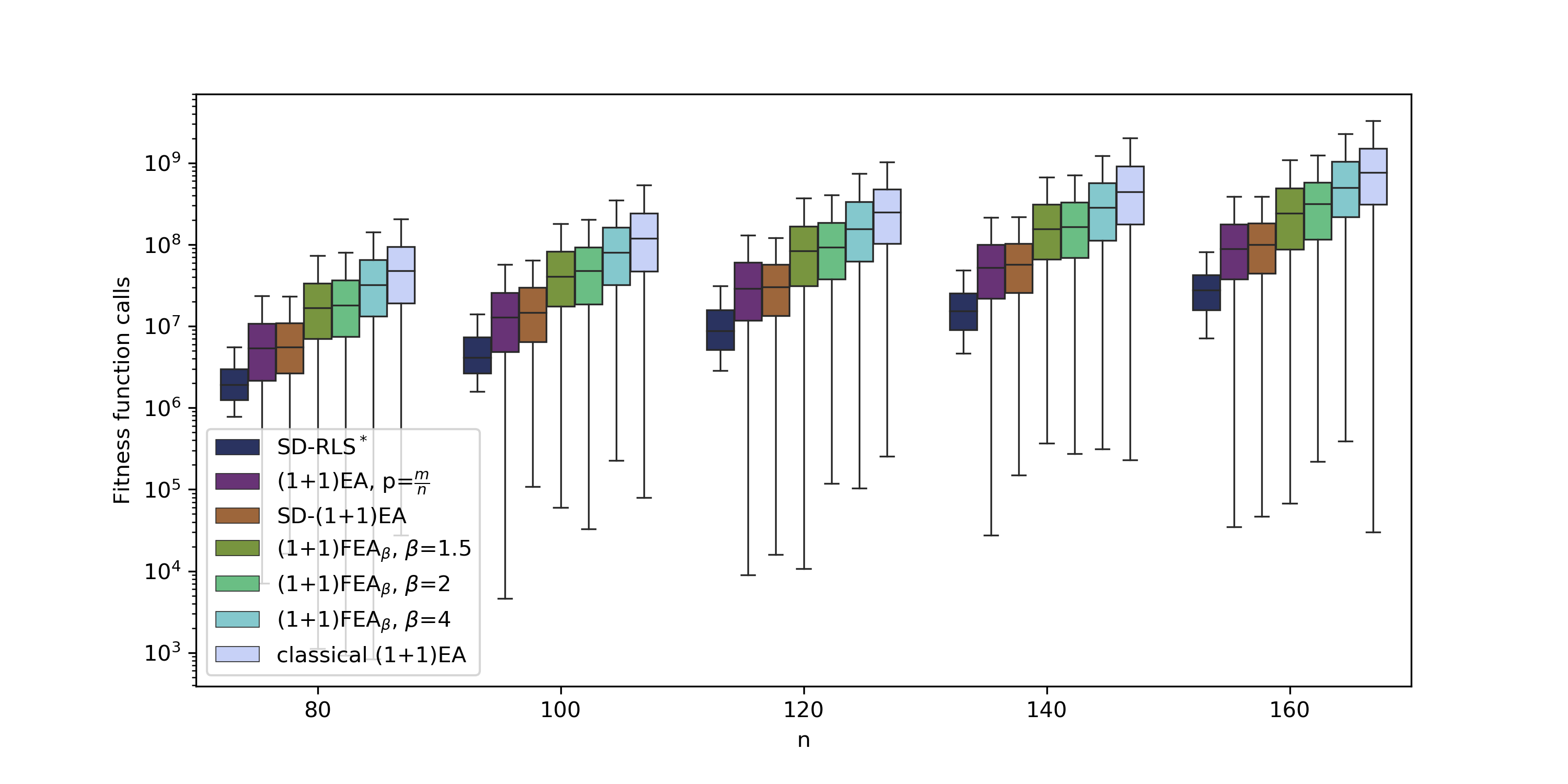
In the first experiment, we ran an implementation of Algorithm 3 (SD-RLS∗) on the Jump fitness function with jump size and varying from 80 to 160. We compared our algorithm against the (1+1) EA with standard mutation rate , the (1+1) EA with mutation probability , Algorithm (1+1) FEAβ from Doerr et al. 2017 with three different , and the SD-(1+1) EA presented in Rajabi and Witt 2020. In Figure 1, we observe that SD-RLS∗ outperforms the rest of the algorithms.
In the second experiment, we ran an implementation of four algorithms SD-RLS∗, (1+1) FEAβ with from Doerr et al. 2017, the standard (1+1) EA and RLS1,2 from Neumann and Wegener 2007 on the MST problem with the fitness function from Neumann and Wegener 2007 for two types of graphs called TG and Erdős–Rényi.

The graph TG with vertices and edges contains a sequence of triangles which are connected to each other, and the last triangle is connected to a complete graph of size . Regarding the weights, the edges of the complete graph have the weight 1, and we set the weights of edges in triangle to and for the side edges and the main edge, respectively. In this paper, we consider . The graph TG is used for estimating lower bounds on the expected runtime of the (1+1) EA and RLS in the literature Neumann and Wegener 2007. In this experiment, we use . As can be seen in Figure 4b, (1+1) FEAβ is faster than the rest of the algorithms, but SD-RLS∗ outperforms the standard (1+1) EA and RLS1,2.


Regarding the graphs Erdős–Rényi, we produced some random Erdős–Rényi graphs with and assigned each edge an integer weight in the range uniformly at random. We also checked that the graphs certainly had a spanning tree. Then, we ran the implementation on MST of these graphs. The obtained results can be seen in Figure 4a. As we discussed in Section 6, SD-RLS∗ does not outperform the (1+1) EA and RLS1,2 on MST with graphs where the number of strict improvements in SD-RLS∗ is large.
For statistical tests, we ran the algorithms on the graphs TG and Erdős–Rényi over 400 times, and all p-values obtained from a Mann-Whitney U-test between the algorithms, with respect to the null hypothesis of identical behavior, are less than except for the results regarding the graph TG with .
Conclusions
We have transferred stagnation detection, previously proposed for EAs with standard bit mutation, to the operator flipping exactly uniformly randomly chosen bits as typically encountered in randomized local search. Through both theoretical runtime analyses and experimental studies we have shown that this combination of stagnation detection and local search efficiently leaves local optimal and often outperforms the previously considered variants with global mutation. We have also introduced techniques that make the algorithm robust if it, due to its randomized nature, misses the right number of bits flipped, and analyzed scenarios where global mutations are still preferable. In the future, we would like to investigate stagnation detection more thoroughly on instances of classical combinatorial optimization problem like the minimum spanning tree problem, for which the present paper only gives preliminary but promising results.
Acknowledgement
This work was supported by a grant by the Danish Council for Independent Research (DFF-FNU 8021-00260B).
References
- Bassin and Buzdalov (2019) Bassin, Anton and Buzdalov, Maxim (2019). The 1/5-th rule with rollbacks: on self-adjustment of the population size in the (1+(,)) GA. In Proc. of GECCO 2019 (Companion), 277–278. ACM Press.
- Corus, Oliveto and Yazdani (2018) Corus, Dogan, Oliveto, Pietro S., and Yazdani, Donya (2018). Fast artificial immune systems. In Proc. of PPSN 2018, vol. 11102 of LNCS, 67–78. Springer.
- Doerr (2020) Doerr, Benjamin (2020). Probabilistic tools for the analysis of randomized optimization heuristics. In Doerr, Benjamin and Neumann, Frank (eds.), Theory of Evolutionary Computation – Recent Developments in Discrete Optimization, 1–87. Springer.
- Doerr and Doerr (2016) Doerr, Benjamin and Doerr, Carola (2016). The impact of random initialization on the runtime of randomized search heuristics. Algorithmica, 75(3), 529–553.
- Doerr and Doerr (2018) Doerr, Benjamin and Doerr, Carola (2018). Optimal static and self-adjusting parameter choices for the (1+(, )) genetic algorithm. Algorithmica, 80(5), 1658–1709.
- Doerr and Doerr (2020) Doerr, Benjamin and Doerr, Carola (2020). Theory of parameter control for discrete black-box optimization: Provable performance gains through dynamic parameter choices. In Doerr, B. and Neumann, F. (eds.), Theory of Evolutionary Computation – Recent Developments in Discrete Optimization, 271–321. Springer.
- Doerr, Doerr and Yang (2016) Doerr, Benjamin, Doerr, Carola, and Yang, Jing (2016). -bit mutation with self-adjusting outperforms standard bit mutation. In Proc. of PPSN 2016, vol. 9921 of Lecture Notes in Computer Science, 824–834. Springer.
- Doerr, Fouz and Witt (2010) Doerr, Benjamin, Fouz, Mahmoud, and Witt, Carsten (2010). Quasirandom evolutionary algorithms. In Proc. of GECCO ’10, 1457–1464. ACM.
- Doerr et al. (2019) Doerr, Benjamin, Gießen, Christian, Witt, Carsten, and Yang, Jing (2019). The (1 + ) evolutionary algorithm with self-adjusting mutation rate. Algorithmica, 81(2), 593–631.
- Doerr, Jansen and Klein (2008) Doerr, Benjamin, Jansen, Thomas, and Klein, Christian (2008). Comparing global and local mutations on bit strings. In Ryan, Conor and Keijzer, Maarten (eds.), Proc. of GECCO ’08, 929–936. ACM Press.
- Doerr, Johannsen and Winzen (2012) Doerr, Benjamin, Johannsen, Daniel, and Winzen, Carola (2012). Multiplicative drift analysis. Algorithmica, 64, 673–697.
- Doerr et al. (2017) Doerr, Benjamin, Le, Huu Phuoc, Makhmara, Régis, and Nguyen, Ta Duy (2017). Fast genetic algorithms. In Proc. of GECCO ’17, 777–784. ACM Press.
- Hansen and Mladenovic (2018) Hansen, Pierre and Mladenovic, Nenad (2018). Variable neighborhood search. In Martí, Rafael, Pardalos, Panos M., and Resende, Mauricio G. C. (eds.), Handbook of Heuristics, 759–787. Springer.
- Lengler (2020) Lengler, Johannes (2020). Drift analysis. In Doerr, B. and Neumann, F. (eds.), Theory of Evolutionary Computation – Recent Developments in Discrete Optimization, 89–131. Springer.
- Lissovoi, Oliveto and Warwicker (2019) Lissovoi, Andrei, Oliveto, Pietro S., and Warwicker, John Alasdair (2019). On the time complexity of algorithm selection hyper-heuristics for multimodal optimisation. In Proc. of AAAI 2019, 2322–2329. AAAI Press.
- Lugo (2017) Lugo, Michael (2017). Sum of ”the first ” binomial coefficients for fixed . MathOverflow. URL https://mathoverflow.net/q/17236. (version: 2017-10-01).
- Neumann and Wegener (2007) Neumann, Frank and Wegener, Ingo (2007). Randomized local search, evolutionary algorithms, and the minimum spanning tree problem. Theoretical Computer Science, 378, 32–40.
- Raidl, Koller and Julstrom (2006) Raidl, Günther R., Koller, Gabriele, and Julstrom, Bryant A. (2006). Biased mutation operators for subgraph-selection problems. IEEE Transaction on Evolutionary Computation, 10(2), 145–156.
- Rajabi and Witt (2020) Rajabi, Amirhossein and Witt, Carsten (2020). Self-adjusting evolutionary algorithms for multimodal optimization. In Proc. of GECCO ’20, 1314–1322. ACM Press.
- Warwicker (2019) Warwicker, John Alasdair (2019). On the runtime analysis of selection hyper-heuristics for pseudo-Boolean optimisation. Ph.D. thesis, University of Sheffield, UK. URL http://ethos.bl.uk/OrderDetails.do?uin=uk.bl.ethos.786561.
- Wegener (2001) Wegener, Ingo (2001). Methods for the analysis of evolutionary algorithms on pseudo-Boolean functions. In Sarker, Ruhul, Mohammadian, Masoud, and Yao, Xin (eds.), Evolutionary Optimization. Kluwer Academic Publishers.
- Witt (2014) Witt, Carsten (2014). Revised analysis of the (1+1) EA for the minimum spanning tree problem. In Proc. of GECCO ’14, 509–516. ACM Press.