POD-DL-ROM: enhancing deep learning-based reduced order models for nonlinear parametrized PDEs by proper orthogonal decomposition
Abstract
Deep learning-based reduced order models (DL-ROMs) have been recently proposed to overcome common limitations shared by conventional reduced order models (ROMs) – built, e.g., through proper orthogonal decomposition (POD) – when applied to nonlinear time-dependent parametrized partial differential equations (PDEs). These might be related to (i) the need to deal with projections onto high dimensional linear approximating trial manifolds, (ii) expensive hyper-reduction strategies, or (iii) the intrinsic difficulty to handle physical complexity with a linear superimposition of modes. All these aspects are avoided when employing DL-ROMs, which learn in a non-intrusive way both the nonlinear trial manifold and the reduced dynamics, by relying on deep (e.g., feedforward, convolutional, autoencoder) neural networks. Although extremely efficient at testing time, when evaluating the PDE solution for any new testing-parameter instance, DL-ROMs require an expensive training stage, because of the extremely large number of network parameters to be estimated. In this paper we propose a possible way to avoid an expensive training stage of DL-ROMs, by (i) performing a prior dimensionality reduction through POD, and (ii) relying on a multi-fidelity pretraining stage, where different physical models can be efficiently combined. The proposed POD-DL-ROM is tested on several (both scalar and vector, linear and nonlinear) time-dependent parametrized PDEs (such as, e.g., linear advection-diffusion-reaction, nonlinear diffusion-reaction, nonlinear elastodynamics, and Navier-Stokes equations) to show the generality of this approach and its remarkable computational savings.
Keywords:
reduced order modeling, deep learning, proper orthogonal decomposition, dimensionality reduction, parametrized PDEs1 Introduction
Performing the numerical approximation of parametrized partial differential equations (PDEs) for multiple parameter values, or solving them in real-time, is unaffordable by means of full order, traditional high-fidelity techniques, such as the Galerkin-finite element method [1]. Replacing a full order model (FOM) by a reduced order model (ROM), featuring a much lower dimension, yet capable to express the physical features of the problem at hand, is the main goal of reduced order modeling techniques, among which the reduced basis (RB) method represents one of the most popular options [2]. The basic assumption underlying the RB method is that the solution of a parametrized PDE lies on a low-dimensional manifold, which can be approximated by a linear trial subspace spanned by a set of basis functions [3, 4], built from a set of FOM snapshots employing, e.g., proper orthogonal decomposition (POD). In this case, the ROM approximation is given by the linear superimposition of POD modes, whose degrees of freedom (depending both on time and parameters) result from the solution of a low-dimensional (nonlinear, dynamical) system, obtained through a (Petrov-)Galerkin projection onto a linear test subspace, which might coincide with the trial subspace. Being able to assemble such a ROM efficiently, for any new parameter instance, is granted at the price of a further hyper-reduction stage on the FOM arrays [5].
ROMs for parametrized PDEs rely on a suitable offline-online computational splitting: computationally expensive tasks required to build the low-dimensional subspace, and assemble all the ROM arrays, are performed once for all during the so-called offline (or ROM training) stage, then allowing to compute – ideally – in an extremely efficient way the ROM approximation for any new parameter value, during the so-called online (or ROM testing) stage.
This computational strategy, however, breaks down if (i) the dimension of the linear trial subspace becomes very large (compared to the intrinsic dimension of the solution manifold being approximated), or (ii) the hyper-reduction stage, required to approximate parameter-dependent nonlinear terms – at the limit, the whole residual vector and, possibly, the Jacobian matrix when dealing with implicit solvers such as, e.g., the Newton method – requires linear subspaces whose dimension becomes very large, too, in order to provide an approximation to FOM arrays sufficiently accurate.
These can be recurrent issues when dealing with nonlinear, time-dependent parametrized PDEs, and (i) we aim at building a ROM able to provide problem approximations uniformly accurate over the whole parameter space, (ii) the parametrized problem features coherent structures (e.g., transport or wave phenomena) that propagate over time and depend on parameters. Last, but not least, ensuring ROM stability might require additional computational efforts, such as, e.g., when dealing with fluid flows using a mixed formulation (e.g., a velocity-pressure formulation for Navier-Stokes equations), see, e.g., [6, 7, 8].
To overcome these drawbacks, we have recently proposed in [9, 10] a strategy to construct deep learning-based ROMs (DL-ROMs) for nonlinear time-dependent parametrized PDEs in a non-intrusive way, exploiting deep neural networks as main building block, and a set of FOM snapshots. In particular, the DL-ROM technique allows approximating both the solution manifold of the PDE by means of a low-dimensional, nonlinear trial manifold, and the nonlinear dynamics of the generalized coordinates on such reduced trial manifold, as a function of the time coordinate and the parameters. Both (i) the nonlinear trial manifold and (ii) the reduced dynamics are learnt in a non-intrusive way, thus avoiding the projection stage typical of the RB method; in particular, the trial manifold is learnt by means of the decoder function of a convolutional autoencoder (CAE) neural network, whereas the reduced dynamics through a (deep) feedforward neural network (DFNN), and the encoder function of the CAE (see Section 3.2 for further details).
DL-ROMs outperform the RB method – even involving local reduced bases – regarding both numerical accuracy (for the same ROM dimension) and computational efficiency during the online (or testing) stage, when applied to problems that are typically challenging for the RB method (such as, e.g., linear transport equation, nonlinear diffusion-reaction equations whose solution develops moving fronts depending on parameters) or problems featuring reduced bases with usually large dimension. A key aspect, still open in the setting of DL-ROMs and which this paper is mainly devoted to, deals with the computational efficiency of DL-ROMs during the offline (or training) stage, which is also related with the curse of dimensionality. Indeed, training the two networks representing the building blocks of the DL-ROM entails a number of networks parameters to be estimated (and, correspondingly, training data dimensions) that blow up with the dimension of the FOM – this latter being related with, e.g., the mesh size required by a Galerkin-finite element approximation of the PDEs. Indeed, DL-ROMs have been applied so far to the reduction of scalar PDEs, with at most degrees of freedom.
In this paper we propose a strategy to enhance DL-ROMs in order to make the offline training stage dramatically faster, allowing for much larger FOM dimensions, without affecting the number of networks parameters to be estimated and, ultimately, network complexity. This strategy exploits (i) dimensionality reduction of FOM snapshots through randomized POD (rPOD) [11], to be considered as the action of the first layer of the CAE, rather than the way to generate the linear trial manifold, as done instead in traditional POD-Galerkin ROMs, and (ii) a suitable multi-fidelity pretraining stage [12], where different models (built, e.g., by considering coarser discretizations or simplified physical models) can be efficiently combined, to iteratively initialize the network parameters.
These substantial enhancements of the DL-ROM technique provide a new way to build deep learning-based ROMs, which we refer to POD-DL-ROM. The resulting strategy represents a suitable combination of the best features of deep learning (DL) algorithms and POD – namely, the non-intrusive character of the former, and the simplicity, combined with the rigorous mathematical foundation, of the latter – at the same time fixing their weaknesses – namely, the curse of dimensionality of DL-ROM for increasing FOM dimensions, and the modest approximation properties of POD-based linear trial manifolds for some classes of nonlinear parametrized PDEs. As a result, the POD-DL-ROM technique provides not only substantial gains during the offline training stage if compared to the DL-ROM strategy – keeping fixed the dimension of the FOM that we used to generate snapshots – but also during the online testing stage, if compared to POD-Galerkin ROMs, also in those cases where this latter technique provides satisfying results in terms of both accuracy and efficiency.
The structure of the paper is as follows. In Section 2 we briefly recall the construction of DL-ROMs by reinterpreting the classical ideas behind linear projection-based methods for parametrized PDEs, comparing our strategy with alternative ways to build ROMs relying on machine/deep learning algorithms. In Section 3 we then describe the POD-DL-ROM technique showing (i) how to enhance the DL-ROM technique by means of (randomized) POD, (ii) how to rely on a multi-fidelity pretraining stage, and (iii) how to generalize this technique to the case of vector problems. In Section 4 we assess the numerical accuracy and efficiency on four different test cases, namely (i) a linear advection-diffusion-reaction problem, (ii) a nonlinear diffusion-reaction problem arising from cardiac electrophysiology, (iii) nonlinear elastodynamics for hyperelastic compressible materials, and (iv) fluid dynamics, also showing the great versatility of the proposed technique.
2 An overview of deep learning-based ROMs
Before introducing the main features of POD-DL-ROMs, we review the construction of DL-ROMs and highlight the main differences between our framework and existing techniques in literature.
2.1 DL-ROMs in a nutshell
For the sake of generality, we consider a generic nonlinear, time-dependent PDE depending on a set of input parameters , where the parameter space is given by a bounded and closed set; input parameters might represent physical or geometrical properties of the system, like, e.g., material properties, initial and boundary conditions, or the shape of the domain. Even if we only consider physical parameters, handling geometrical parameters does not require additional efforts. We adopt a fully algebraic perspective and assume to start from the high-fidelity (spatial) approximation of the PDE, which we refer to as full order model (FOM). Regardless of the spatial discretization adopted – such as, e.g., the finite element method, Isogeometric Analysis or the spectral element method – the FOM can be expressed as a nonlinear parametrized dynamical system. Hence, given , we aim at solving the initial value problem
| (1) |
where:
- -
is the parametrized solution of (1);
- -
is the initial datum;
- -
is a (nonlinear) function, encoding the system dynamics;
- -
is the parametric, mass matrix of this parametric FOM; without any loss of generality, is assumed here to be a symmetric positive definite matrix.
The FOM dimension is related with the finite dimensional subspaces introduced for the sake of space discretization – here denotes a discretization parameter, such as the maximum diameter of elements in a computational mesh; consequently, can be extremely large if the PDE problem describes complex physical behaviors and/or high degrees of accuracy are required to its solution. In order to solve problem (1), suitable time discretizations are employed, such as backward differentiation formulas (BDFs) [1] and generalized- [13] methods. We thus aim at approximating, in an efficient way, the set
| (2) |
of solutions to problem (1) when varies in , also referred to as solution manifold.
If for any , problem (1) admits a unique solution, for each , the intrinsic dimension of the solution manifold is at most , where is the number of parameters (time plays the role of an additional coordinate). In this case, each element can be described in terms of at most intrinsic coordinates, even if their explicit characterization is, in practice, computationally unaffordable. Equivalently, the tangent space to the manifold at any given is spanned by basis vectors.
When dealing with traditional projection-based ROMs, the approximated solution to (1) is sought in the subspace of dimension , spanned by the columns of . Hence, a linear ROM looks for an approximation of the form
| (3) |
where . Hence, the reduced linear trial manifold is given by
| (4) |
In POD-Galerkin ROMs, is spanned by the first singular vectors of
| (5) |
a matrix collecting FOM solutions (or snapshots) computed for different parameter values , suitably sampled11 1 Sampling frequency in time does not necessarily coincide with the time stepping rule used to discretize in time (1); similarly, singular value decomposition can be done either on , or following a two-stage procedure, operating SVD across samples in time for each , , and then on the resulting collection of selected singular vectors. over the parameter space, at different time instants .
In the POD-Galerkin case, to model the reduced dynamics of the system, we replace by (3) in system (1), and impose that the residual
| (6) |
is orthogonal to . This condition yields the following POD-Galerkin ROM
| (7) |
where:
- -
is the reduced mass matrix;
- -
;
- -
is the initial condition for associated with the initial condition for , where we have assumed, without loss of generality, that .
The two main bottlenecks often arising with POD-Galerkin ROMs are (i) the increasing dimension of the low-dimensional POD subspaces, much larger than the intrinsic dimension of the solution manifold, and (ii) the need to rely on hyper-reduction techniques to assemble the operators appearing in the ROM (7) in order not to rely on expensive -dimensional arrays [5].
DL-ROMs have been introduced in [9] to overcome these limitations of POD-Galerkin ROMs, and further applied to cardiac electrophysiology in [10]. A DL-ROM describes both the trial manifold and the reduced dynamics (corresponding to the matrix and the projection stage, respectively, in the POD-Galerkin case) through deep neural networks, which are trained on a set of FOM snapshots. In this way, DL-ROMs completely avoid the projection stage, are non-intrusive, and can be cheaply evaluated once trained. In particular:
- 1.
to describe the system dynamics on a suitable reduced nonlinear trial manifold (a task which we refer to as reduced dynamics learning), the intrinsic coordinates of the ROM approximation are defined as
(8) where is a DFNN, consisting in the subsequent composition of a nonlinear activation function, applied to a linear transformation of the input, multiple times [12]. Here denotes the vector of parameters of the DFNN, collecting all the corresponding weights and biases of each layer of the DFNN;
- 2.
to model the reduced nonlinear trial manifold (a task which we refer to as reduced trial manifold learning) we employ the decoder function of a CAE [14, 15], that is,
(9) where denotes the decoder function of a CAE obtained as the composition of several layers (some of which are convolutional), depending upon a vector collecting all the corresponding weights and biases.
The DL-ROM approximation is then given by
| (10) |
The encoder function of the convolutional AE, provided when carrying out its training on the FOM snapshots, can then be exploited to map the FOM solution associated to onto a low-dimensional representation
| (11) |
denotes the encoder function, depending upon a vector of parameters.
Computing the DL-ROM approximation of , for any possible and , corresponds to the testing stage of a DFNN and of the decoder function of a convolutional AE; this does not require the evaluation of the encoder function. The training stage consists in solving the following optimization problem, in the variable , after the snapshot matrix has been formed:
| (12) |
where and
| (13) |
where
with . The per-example loss function (13) combines the reconstruction error (that is, the error between the FOM solution and the DL-ROM approximation) and the error between the intrinsic coordinates and the output of the encoder.
2.2 The content of this paper and other existing approaches
Several recent works have shown possible applications of DL algorithms for solving PDEs – thanks to their ability of effectively approximating nonlinear maps, and by their ability to learn from data and generalize to unseen data – both from a theoretical [16, 17, 18] and a computational standpoint. Regarding this latter, we mention, for instance, physics-informed neural networks (PINNs) [19, 20, 21, 22] or physics-informed deep generative models [23, 24]. DL algorithms and artificial neural networks (ANN), such as feedforward neural networks, are becoming more and more popular in reduced order modeling, too. In particular:
- 1.
ANNs have been employed to model the reduced dynamics in a data-driven and less intrusive way (avoiding, e.g., the costs entailed by the projection stage of projection-based ROMs); for instance, in [25, 26, 27, 28, 29] the use of ANNs or Gaussian Processes (GPs) regression models has been proposed to approximate the mapping from the input parameters (and, possibly, time) to the reduced coefficients, as an alternative to the assembly and solution of the reduced order system arising from POD-Galerkin ROMs, however still using a linear trial manifold built through POD; similar strategies have also been introduced in [30, 31, 32, 33, 34]. A hybrid strategy proposed in [35] merges ANN-based regression models and PINNs, training the network by minimizing the mean squared residual error of the reduced order equation on a set of points in parameter space; similar results can be found in [36]. Moreover, feedforward and recurrent neural networks have been exploited in [37, 38] to address closure problems and model the effects of discarded modes on the set of retained POD modes. Very recently, an ANN-based methodology is proposed to learn mappings between infinite-dimensional spaces for parametric PDEs in [39], exploiting POD and showing mesh-independent properties.
- 2.
ANNs have been used to describe the reduced trial manifold where the approximation is sought (thus avoiding the linear superimposition of POD modes), either relying on a minimum residual formulation to derive the ROM [40, 41], or without considering an explicit parameter dependence in the differential problem that is considered [42]. For instance, projection-based ROMs are built in [40] by performing a projection of the FOM onto a nonlinear trial manifold identified by means of the decoder function of a CAE – hence, still requiring the assembling and the solution of a ROM as in traditional POD-Galerkin ROMs. The use of CAEs has also been proposed in [42], where a reduced trial manifold is generated through a deep convolutional recurrent AE, which is then used to train a Long Short-Term Memory (LSTM) neural network that models the reduced dynamics.
Our DL-ROM approach [9, 10] combines and improves the techniques introduced in [42, 40]. As detailed in Section 2.1, the (i) nonlinear trial manifold is learnt by using the decoder function of a CAE, while (ii) the dynamics on the reduced manifold is modeled through a DFNN and the encoder function of a CAE. These two tasks are achieved simultaneously, by training both the CAE and the DFNN network architectures at the same time, by minimizing a loss function weighting two terms – see (13) – one for each task. The resulting procedure thus avoids both the expensive projection stage of [40] and the training of a more expensive LSTM network [42]. Moreover, the DL-ROM technique is purely data-driven, non-intrusive: it only relies on the computation of a set of FOM snapshots. In this respect, DL does not replace the high-fidelity FOM as, e.g., in the works by Karniadakis and coauthors [19, 20, 21, 22, 43]; rather, DL techniques are built upon it, to enhance the repeated evaluation of the FOM for different values of the parameters. The computational benefits introduced by the use of DL-ROMs can be summarized as follows:
- 1.
the dimension of the DL-ROM can be kept extremely small, very close (or even equal) to the dimension of the solution manifold ;
- 2.
the DL-ROM can be queried at any desired time instant, without requiring the solution of a dynamical system until that time, differently from projection-based ROMs such as, e.g, POD-Galerkin ROMs;
- 3.
the time resolution required by the DL-ROM can be chosen to be larger than the one required by the numerical solution of dynamical systems at hand (see, e.g., [10]);
- 4.
DL-ROMs avoid the use of (intrusive and very often extremely expensive) hyper-reduction techniques, which are instead required by POD-Galerkin ROMs;
- 5.
DL-ROMs can avoid to account for those auxiliary variables of a problem which we might not be interested into (as pressure, compared to velocity, in fluid flow problems, or the gating variables, compared to the electric potential, in cardiac electrophysiology [10]).
For all these reasons, DL-ROMs tremendously improve the computational efficiency of ROMs during the online testing stage. However, the offline training stage of DL-ROM would still depend on , a fact which ultimately might entail overwhelming training times and costs when is moderately large.
The POD-DL-ROM technique proposed in this work, thanks to a prior dimensionality reduction relying on POD and a suitable multi-fidelity pretraining, greatly enhances the efficiency of the DL-ROM during the training phase, thus dramatically decreasing training computational times, as shown by the numerical results discussed in following Sections.
3 A new deep learning-based reduced order model
POD-DL-ROMs provide a new, general-purpose, ROM approach combining a data dimensionality reduction obtained through POD with the DL-ROM approach [9, 10]. After introducing the POD-DL-ROM approach, we discuss in more details some of its building blocks, the extension to vector problems, finally reporting detailed algorithms for the offline (or training) and the online query (or testing) stages.
3.1 POD-enhanced DL-ROMs (POD-DL-ROMs)
The POD-DL-ROM technique consists in applying the DL-ROM technique to the intrinsic coordinates of a linear trial manifold generated through randomized singular value decomposition (rSVD) and approximating ; alternatively, it can be seen as a ROM technique in which a two-step dimensionality reduction is performed: first, POD (realized through rSVD) is applied on a set of FOM snapshots, then a DL-ROM is built to approximate the map between and the POD generalized coordinates. In this way, all the DL-ROM features allowing its very efficient testing time are retained. As a matter of fact, as shown in Section 2.1, DL-ROMs might imply overwhelming training costs (and times) when the FOM dimension becomes moderately large, although remaining extremely efficient at testing time. We emphasize that very often ROMs are designed to be efficient only regarding their online performances, no matter how expensive is the offline stage. Our (more ambitious) goal is instead to realize a ROM able of efficient computational performance during both offline and online stages, compared to classical projection-based ROMs.
Using randomized POD (see Section 3.2), we first build the -dimensional subspace spanned by the columns of , the matrix of the first singular vectors of the snapshot matrix . We denote the dimension of the linear manifold by , to distinguish it from the dimension of the nonlinear trial manifold, and to emphasize that this dimension can be taken (much) larger with respect to the one of the reduced linear trial manifold that would have been exploited in a POD-Galerkin ROM. Indeed, here linear dimensionality reduction is performed only for the sake of data compression, to avoid to feed training data of dimension .
The POD-DL-ROM approximation of the FOM solution is given by
that is, it is sought in a linear trial manifold22 2 Equivalently, we have replaced the original solution manifold with the -dimensional linear manifold As in the case of , the intrinsic dimension of is at most . of (potentially large) dimension ,
| (14) |
by applying the DL-ROM strategy of Section 2.1 to approximate – rather than . The DL-ROM approximation takes the form
| (15) |
and is sought in a reduced nonlinear trial manifold of dimension . By adapting the DL-ROM formulation of Section 2.1 to the case at hand, we have that:
- 1.
to describe the system dynamics on the nonlinear trial manifold – with as close as possible to – the intrinsic coordinates of the approximation are defined as
where is a DFNN;
- 2.
to model the reduced nonlinear trial manifold , we employ the decoder function of a CAE, that is,
(16) where .
The encoder function of the convolutional AE can then be exploited to map the intrinsic coordinates associated to onto a low-dimensional representation
where denotes the encoder function, depending upon a vector of parameters.
The architecture of the POD-DL-ROM neural network, employed at training time, is the one shown in Figure 1; note that, at testing time, as in the DL-ROM technique we can discard the encoder function.

Computing the ROM approximation (15) by means of a POD-DL-ROM thus consists in solving the optimization problem (12) where the per-example loss function (13) is now replaced by
| (17) |
where
We point out that the POD-DL-ROM technique relies on a further level of dimensionality reduction compared to [27, 29], since the dimension of the reduced linear problem – that is, the number of intrinsic coordinates included in – is decreased until (almost, or exactly) matching the intrinsic dimension of the parametrized problem. In addition, we introduce the use of convolutional layers, which results better suited to high-dimensional spatial data, thus implying lower computational costs, with respect to dense layers. Moreover, the POD-DL-ROM approach allows to model and approximate the entire intrinsic coordinates vector all at once, without requiring additional SVDs, if compared to the data-driven RB method, employing GPs as regression models, proposed in [26] and further extended in [28].
We highlight that by shaping the POD-DL-ROM neural network as a zero-extended neural network and assuming that the input-output map is locally Lipschitz, it is possible to prove the convergence of the framework here proposed by following the approach presented in [39].
3.2 (Randomized) POD for dimensionality reduction
Even though POD is not able to generate linear subspaces whose dimension is close to (or matches) the intrinsic dimension of the problems under consideration, it is still able to perform a moderate dimensionality reduction, thus yielding a linear subspace of dimension . However, computing the SVD of the snapshot matrix can be extremely time consuming for large-scale problems; whenever dealing with FOMs of moderately large dimension and/or a high number of training-parameter or time instances, the computational time and memory required by SVD may become prohibitive, scaling superlinearly in and [44]. In order to speed up computations, we rely on the randomized matrix approximation techniques developed in [45]; in particular, we exploit rSVD, which computes an approximated SVD, using randomization.
More precisely, a Gaussian random matrix is drawn, where ; is called the oversampling parameter. The matrix
is then assembled, by normally setting or 2; then, an iterative QR factorization , is computed, where . Computing in such a way consists of applying an adaptive randomized range finder algorithm to approximate the range of by means of a matrix whose columns are orthonormal, i.e. [45]. Once the matrix has been computed, it is restricted to the first columns, denoted by , and the SVD of the matrix
| (18) |
is computed. The SVD factorization of is then recovered by setting
| (19) |
The rSVD approximation can then be computed through the following steps:
- 1.
an approximated basis for Col(), i.e. , is obtained by using randomization,
- 2.
the SVD of the matrix in (18) is computed,
- 3.
the matrix is recovered by means of as in (19).
We refer to as to the rPOD basis matrix. For further details about rSVD we refer to [45, 11].
3.3 Pretraining
Directly training a model to solve a specific task can be very demanding if the model is complex and hard to optimize, and/or the task is very difficult. More viable options are either (i) to train a simpler model to solve the task, then make the model more complex, or (ii) to train the model to solve a simpler task, then move on to the final task. Both these strategies are known in the DL literature as pretraining [12]. In particular, a finer tuning of a pretrained model is equivalent to transfer learning, if the data used to perform fine tuning are of different nature with respect to the data used during pretraining. Pretraining can then be seen as a form of transfer learning, where a pretrained model is used as initial state of the network [46]; this strategy works extremely well in many objects classification tasks [47] and natural language processing problems [48]. In the area of scientific ML, pretraining has been used, for instance, in [49] where a pretrained neural network has been used to perform parameter identification on a new dataset.
Relying on a suitable pretraining, we are able to further enhance the training phase of a POD-DL-ROM, combining models of different fidelities (e.g., by considering coarser/finer spatial discretizations, as well as different physical laws, more/less parameters or larger/smaller parameter ranges). In particular, we train the POD-DL-ROM neural network on an initial simpler task, obtaining a set of parameters , and then use them to initialize the training of the POD-DL-ROM neural network on a more complex problem, by setting . Numerical results of Section 4 will show how pretraining, combined with the dimensionality reduction obtained through rPOD, represents a cornerstone in view of drastically reducing the training computational time of a POD-DL-ROM, if compared to the time required for training, from scratch, a neural network on the more complex task.
3.4 Extension to vector problems
Compared to the DL-ROM technique, applied so far to scalar problems only, we have further generalized the POD-DL-ROM technique in order to handle vector problems, in analogy to what happens when treating red-green-blue (RGB) images in general. DL algorithms. By considering the spatial discretization of a vector PDE problem, whose solution is a -dimensional vector field, problem (1) can be rewritten as
| (20) |
where is the solution of the -th equation in (20), is the -th initial datum, describes the dynamics of , , with . Depending on the problem at hand, some of the equations appearing in (20) might not involve the derivatives and related initial conditions; this is what happens, for instance, in the case of unsteady Navier-Stokes equations for incompressible flows, where the equation expressing flow incompressibility involves the velocity components, but no time derivatives.
Provided the solution of (20), associated to a particular instance , and the orthonormal basis , with , found though rSVD, we compute the intrinsic components , reshape each component in a square matrix of dimension , where with , and stack them together forming a tensor with channels. Thus, each vectorial component of the solution of problem (20) is reshaped in a square matrix; then, they are stacked together forming a tensor of dimension .
This approach allows the dimensions , , of each FOM component, to be different. Indeed, it is the rPOD dimension used to reduce each vector component that must be kept equal for . We remark that by stacking all components together allows to reduce the number of parameters, and then the training and testing computational times of POD-DL-ROM.
3.5 Training and Testing Algorithms
We summarize in this section both the training and the testing stage of the POD-DL-ROM technique. Regarding the setting of the optimization algorithm, the way to select the hyperparameters and the architecture of the neural networks, we refer to [9, 10]. We denote by the matrix collecting all the parameter instances corresponding to the computed snapshots; these latter are included in the snapshot matrix , defined in (5). Note that, in the case of a vector problem, the snapshot matrix takes the form
The input and the output of the POD-DL-ROM are normalized by applying to each channel of the -dimensional tensor the affine transformation detailed below. After splitting the data in and – where , and is a user-defined training-validation splitting fraction – we define
| (21) |
so that parameters are normalized by applying the following transformation
| (22) |
that is, each feature of the training parameter matrix is rescaled according to its maximum and minimum values. Regarding instead the training snapshot matrix , we define
| (23) |
and apply transformation (22), by replacing with respectively, to each channel of – that is, we use the same maximum and minimum values for all the features of the snapshot matrix, as in [40, 42]. Using the latter approach or employing each feature’s maximum and minimum values, for the matrix , does not lead to remarkable changes in the POD-DL-ROM performance. Transformation (22) is applied also to the validation and testing sets, but considering as maximum and minimum the values computed over the training set. In order to rescale the reconstructed solution to the original values, we apply the inverse transformation of (22).
We detail the algorithms through which the training and the testing of the neural network are performed in Algorithms 1 and 2. During the training phase, the optimal parameters of the POD-DL-ROM are found by solving the optimization problem (12)-(17) through the back-propagation and ADAM algorithms (see Algorithm 1). At testing time, the encoder function is instead discarded (see Algorithm 2). By exploiting an early stopping criterion, we stop the training if the loss function does not decrease over a certain number of epochs over the validation set.
We remark that with we refer to a matrix collecting in its columns the output of the encoder function of the convolutional AE applied to each column of the snapshot matrix . In the same way, the columns of collect the minimal coordinates, output of the DFNN, for each sample in the parameter matrix , and is a matrix whose columns are the intrinsic coordinates approximations, outputs of the decoder function of the convolutional AE, associated to the columns of .
4 Numerical results
We assess the numerical performance of the proposed POD-DL-ROM technique, by focusing on the training and testing computational times required to construct and deploy a POD-DL-ROM, and the use of pretraining, on four different linear or nonlinear parametrized PDE problems: (i) a linear unsteady advection-diffusion-reaction equation; (ii) the monodomain system for cardiac electrophysiology; (iii) a nonlinear elastodynamics problem, and (iv) the unsteady Navier-Stokes equations for incompressible flows.
To evaluate the performance of the POD-DL-ROM technique, we rely on two error indicators:
- 1.
the error indicator given by
(24) - 2.
the relative error , for , defined as
(25)
The coefficient in (17) is set equal to 0.5 according to the results shown in [9], where a detailed analysis suggested to select values of equidistant from the extrema of . The rPOD dimension is selected, in all test cases, in such a way that , whereas the dimension of the nonlinear trial manifold is set trying to match the dimension of the solution manifold . The POD-DL-ROM neural network is implemented by means of the Tensorflow DL framework [50].
4.1 Test 1: unsteady advection-diffusion-reaction equation
The first test case we consider deals with the solution of the following advection-diffusion-reaction system
| (26) |
in the two-dimensional domain , where
and
We consider parameters, belonging to ; we build a FOM considering a space discretization made by linear finite elements, considering DOFs, and a Backward Differentiation Formula (BDF) of order 2 considering a time step over with , as time discretization. For different values of and , the solution of (26) exhibits different patterns, due to the location of the distributed source; the dependence on and impact instead on the relative importance of diffusion and advection terms, and on the direction of this latter. We expect that, for the case at hand, POD-Galerkin ROMs might involve a large number of basis functions, also because; note also that the dependence of the solution on and is nonlinear (that is, the problem is nonaffinely parametrized).
Regarding the construction of the proposed POD-DL-ROM, for the training of the neural networks, we consider time instances and training-parameter instances, uniformly distributed in each parametric direction. At testing phase, testing-parameter instances have been considered instead, different from the training ones. The maximum number of epochs is set equal to , the batch size is and, regarding the early-stopping criterion, we stop the training if the loss function does not decrease within 500 epochs. We set as dimension of the rPOD basis (i.e. the linear trial manifold generated by means of rSVD), and as dimension of the reduced nonlinear trial manifold. The training and testing phases of the POD-DL-ROM neural network have been performed on a Tesla V100 32GB GPU.
In Figure 2 we show the FOM and the POD-DL-ROM solutions, for the testing-parameter instances and at , respectively, together with the relative error (25).


The comparison between some components of the intrinsic coordinates vector and their POD-DL-ROM approximation, for the testing parameter instance , is shown is Figure 3. We remark that, as expected, the first components are the ones retaining most of the energy of the system; thus being the ones with higher magnitude [2].


In Figure 3 (right) we show the CPU times, as function of , required by (exact) SVD and rSVD to compute the linear POD space, and thus performing the first level of dimensionality reduction required by the POD-DL-ROM. The CPU time required by SVD is not affected by , while the one required by rSVD increases with respect to – note that the two times almost coincide for , a dimension for which constructing a ROM could in principle be avoided. Hence, rSVD is always preferable with respect to SVD; in particular, for the choice , using rSVD allows a speed-up equal to 32 with respect to SVD.
The trend of the relative error (25) over time, for the selected testing-parameter instance , is displayed in Figure 4 (left), where the mean (over the domain), the median, the first and third quartile of the relative error, as well as its minimum, are reported. The interquartile range (IQR) shows that the distribution of the error is almost uniform over time.
We also analyze the convergence properties of the POD-DL-ROM by varying the number of training-parameter instances provided to the neural network. In particular, in Figure 4 (right) we report the trend of the error indicator (24), over the testing set, versus , i.e. the size of the training dataset. With we refer to the value of the error indicator obtained by setting the maximum number of epochs equal to , which are the iterations performed during the training phase by considering . By increasing , that is by providing more data to the POD DL-ROM neural network, its approximation capability increases, thus yielding a decrease in the error indicator. In particular, the error indicator (25) decays with a rate that is about .


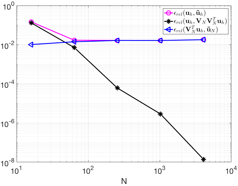
We finally assess the accuracy and the efficiency of the POD-DL-ROM with respect to the dimension of the POD space. In Figure 5 (left) we display the error indicator (24) computed on the FOM and POD-DL-ROM solutions, on the FOM and the optimal-POD (i.e., the projection of the FOM solution onto the linear trial manifold generated through rSVD) solutions, the intrinsic coordinates , and the approximated ones . The trend of , for , is dictated by the projection error , thus indicating that, for , the rPOD dimension is too small to accurately reconstruct the FOM solution. For , the error indicator remains almost unchanged, and almost coincide with . As observed for the DL-ROM [9], this behavior is related to the fact that an increase of only implies the addition of few parameters to the POD-DL-ROM neural network, i.e. the approximation capability of the network remains almost the same while the input increases, thus resulting in a more difficult task.
The GPU training and testing computational times versus are pointed out in Figure 5 (right). The training time refers to the total time required for the training and validation phases; for the sake of completeness we also show the number of epochs along with . The training time varies between 2 h 30 m and 4 h 40 m, we remark that we deal with training-parameter instances. The testing time consists instead in the time required to compute time instances for a testing-parameter instance. The trend is proportional to and, for example, for the testing time is equal to 4.2 s thus leading to a speed-up with respect to the solution of the FOM on a MacBook Pro Intel Core i7 6-core with 16 GB RAM.

4.2 Test 2: coupled PDE-ODE Monodomain/Aliev-Panfilov system
We now consider a coupled PDE-ODE nonlinear system modeling the electrical behavior of the cardiac tissue, from the cellular scale to the tissue level: the Monodomain equation [51] coupled with the Aliev-Panfilov ionic model [52], in a square slab of tissue cm:
| (27) |
We consider two parameters, consisting in the electric conductivities in the longitudinal and the transversal directions to the fibers, i.e., the conductivity tensor takes the form
| (28) |
where and the parameter space is cm2/ms. The applied current is defined as
where mA, , cm2 and ms. The parameters of the Aliev-Panfilov ionic model are set to , , , , , and , see, e.g., [53]. The equations have been discretized in space through linear finite elements by considering grid points. For the time discretization and the treatment of nonlinear terms, we use a one-step, semi-implicit, first order scheme (see, e.g., [54] for further details) by considering a time step ms over the interval , with ms.
For the training phase, we uniformly sample time instances in the interval and consider training-parameters, i.e. with . For the testing phase, testing-parameter instances have been considered, each of them given by with . The maximum number of epochs is , the batch size is and, regarding the early-stopping criterion, we stop the training if the loss function does not decrease within 500 epochs. The simulations are performed on a GTX 1070 8GB GPU. We considered problem (27) first in [9] and we now compare the increased efficiency entailed by the use of POD-DL-ROM compared to a DL-ROM and to a POD-Galerkin ROM.
In Figure 6 we report the FOM and POD-DL-ROM solutions, the latter obtained by setting and , along with the relative error (25), for the testing-parameter instance cm2/ms at ms (top) and ms (bottom).


We point out that setting in (17) equal to 0.5, that is, performing a second level of dimensionality reduction by matching the dimension of the minimal components of the problem, leads to higher accuracies with respect to the case . In this respect, in Table 1, we show the values of the error indicator , over the testing set, by solving the optimization problem (12) with and without considering the term in (17). In particular, setting allows to halve the error.
The comparison among the DL-ROM and POD-DL-ROM neural networks number of parameters, the GPU training and validation time for one epoch, the total number of epochs, the total GPU training and validation (total time) and testing GPU computational times, and the speed-up obtained, at testing time, with respect to the solution of the FOM33 3 The FOM simulation is carried out on a MacBook Pro Intel Core i7 6-core with 16 GB RAM. are reported in Table 2. We also report the total CPU offline and online computational times44 4 Here we employ a full 64 GB node (20 Intel® Xeon® E5-2640 v4 2.4GHz cores) of the HPC cluster available at MOX, Politecnico di Milano. required by the POD-Galerkin ROM with clusters, which corresponds to the choice providing the most efficient results (see, e.g., Test 4 of [9]), by keeping for all the models the same degree of accuracy and running the code on the hardware it is optimized for.
The use of a POD-DL-ROM not only entails even faster testing computational times with respect to a DL-ROM, due to the remarkable reduction of the number of parameters of the neural network, but also reduces the training time of a factor 37.5 (resp. 5) compared to a POD-Galerkin ROM (resp. a DL-ROM). The POD-DL-ROM thus results to be the most efficient ROM both at training and testing stages.
| params | train - val | epochs | total time | test | speed-up | |
| DL-ROM (GPU) | 2342595 | 7.5 - 0.8 | 6981 | 15 h | 0.08 | |
| POD-DL-ROM (GPU) | 269057 | 1.5 - 0.15 | 866 | 24 m | 0.015 | |
| POD-Galerkin ROM () | - | - | - | 115 m | 8 |
We now investigate the use of pretraining, introduced in Section 3.3, in two different scenarios:
- 1.
when increasing the FOM dimension ;
- 2.
when increasing the dimension of the parameter space .
First, we use the optimal parameters, weights and biases, of the POD-DL-ROM neural network found in the case of a FOM dimension , to initialize the POD-DL-ROM neural network parameters associated to two larger FOM dimensions, and , by fixing as rPOD dimension, for a prescribed degree of accuracy . The use of pretraining is possible in this framework because the POD-DL-ROM neural network does not depend on , but only on . Pretraining then allows to reduce the GPU training computational times of a factor , as shown in Table 3, where we compare the training times, in presence of pretraining, with the ones of the network trained from scratch. Irrespectively of pre-training, testing computational times increase with respect to the case due to the dependence on of the matrix-vector product required to recover the final POD-DL-ROM approximation, since has a higher number of rows.
| params | epochs | total time | test | |
| POD-DL-ROM () | 269057 | 1378 | 38 m | 0.06 |
| POD-DL-ROM PRETRAINED | 269057 | 165 | 5 m | 0.06 |
| POD-DL-ROM () | 269057 | 1540 | 42 m | 3 |
| POD-DL-ROM PRETRAINED () | 269057 | 461 | 12 m | 3 |
Then, we report the results referred to a larger parameter space, in the case and . In particular, we use the optimal weights associated to cm2/ms as initial guess of the POD-DL-ROM neural network parameters in the case cm2/ms. We show the GPU training computational times in Table 4 for a prescribed level of accuracy, i.e. , and a fixed number of training-parameter instances , using pretraining and not, respectively. Once again, the use of pretraining allows us to speed up the construction of a POD-DL-ROM remarkably.
| params | epochs | total time | test | |
| POD-DL-ROM | 269057 | 1486 | 41 m | 0.015 |
| POD-DL-ROM PRETRAINED | 269057 | 588 | 16 m | 0.015 |
4.3 Test 3: nonlinear elastodynamics for hyperelastic compressible materials
We now consider the solution of an elastodynamics problem, consisting of the following initial/boundary-value problem [55] for nonlinear elasticity equations, in a three-dimensional beam cm:
| (29) |
Here we consider kg/cm3, kg/(cm s2), and . We consider a St. Venant-Kirchhoff constitutive law involving a hyperelastic nonlinear model to describe the behavior of compressible materials [56], characterized by the following strain energy function
Here is the Green-Lagrange strain tensor, is the deformation tensor defined in terms of the displacement , and are the Lamé coefficients, and
is the first Piola-Kirchhoff stress tensor. Here parameters are considered, given by the Young modulus and the Poisson ratio , belonging to the parameter space ; they affect the expression of the Lamé coefficients as follows
Equations (29) are discretized in space by means of quadratic finite elements, yielding a dynamical system of dimension . For time integration, we use the generalized- method [13] over the interval , with s and a time-step s.
We consider time instances over , training-parameter instances , for and , and testing-parameter instances , for and . We set the rPOD dimension to for each of the three components of the displacement and the dimension of the nonlinear trial manifold to , for a total number of degrees of freedom of the POD-DL-ROM solution equal to 3. The maximum number of epochs is , the batch size is and, regarding the early-stopping criterion, we stop the training if the loss function does not decrease along 500 epochs. The training and testing phases are performed on a GTX 1070 8GB GPU.
In Figure 8 we report the FOM and the POD-DL-ROM solutions, obtained by choosing , and the three components of the displacement vector over the longitudinal axis, i.e. the line which connects the two points cm and cm, for the testing-parameter instance at s. We remark that all the three components are accurately captured by the POD-DL-ROM. In Figure 7 we show the FOM solution and the POD-DL-ROM one, with , along with the relative error (25), for the testing-parameter instance at s. The maximum relative error, which is associated to the portion of the domain undergoing the maximum displacement, is about .


Here we also want to investigate how the use of pretraining involving different fidelity models impacts on the POD-DL-ROM technique, starting from the previous low-fidelity model. In particular, we consider the nearly-incompressible Neo-Hookean constitutive law [56], an hyperelastic nonlinear model whose strain energy function is specified in terms of an isochoric-volumetric splitting
where , , is the shear modulus and the bulk modulus. The coefficients and depend on the Young modulus and the Poisson coefficient and are defined as follow
For this model, we consider parameters, belonging to the parameter space , and an external force ; moreover, the final time is s, that is, we enlarge the time interval, and the time-step is set equal to s. We consider time instances over , training-parameter instances and testing-parameter instances uniformly distributed over the parameter space. We use the optimal weights and biases found on the first low-fidelity model, as initial guess for the parameters of the POD-DL-ROM on this second configuration which thus features (i) a more involved constitutive law, (ii) a different parameter space which reflects in larger displacements, and (iii) a longer time interval where to compute the dynamics.
In Figure 9 we show the FOM and DL-ROM solutions, with , together with the relative error (25), for the testing-parameter instances and at s. In Figure 10 we compare the FOM and POD-DL-ROM, displaying the three components of the displacement vector over the longitudinal axis, for the testing-parameter instance at s.


In Table 5 we finally compare the GPU total and testing computational times of the POD-DL-ROM neural network with and without the use of pretraining. In particular, the use of pretraining allows to strongly reduce the total training and validation time. The testing computational time, which refers to the time needed by the POD-DL-ROM to compute time instances for a testing-parameter instance, is equal to 0.006 s, and is remarkably lower than the final time s, that is our technique is able to return even faster than real-time solutions. In particular, the testing time reflects in a speed-up, if we consider the time required by the solution of the FOM55 5 The simulation is performed on 20 cores of 1.7 TB node (192 Intel® Xeon Platinum® 8160 2.1GHz cores) of the HPC cluster available at MOX, Politecnico di Milano., equal to .
| params | epochs | total time | test | |
| POD-DL-ROM | 270259 | 6490 | 63 m | 0.006 |
| POD-DL-ROM PRETRAINED | 270259 | 1519 | 15 m | 0.006 |
4.4 Test 4: unsteady Navier-Stokes equations
We finally focus on the unsteady Navier-Stokes equations [1] for incompressible flows in primitive variables (fluid velocity and pressure ), considering the flow around a cylinder test case, a well-known benchmark for the evaluation of numerical algorithms for incompressible Navier-Stokes equations in the laminar case:
| (30) |
The domain consists in a two-dimensional pipe with a circular obstacle, i.e. with radius (see Figure 11 for a sketch of the geometry); the boundary is given by , where , being the ball of radius centered at , , and , while denotes the (outward directed) normal unit vector to . We denote by the fluid density, and by the stress tensor,
Here denotes the dynamic viscosity of the fluid, while is the strain tensor,

The density of the fluid is , no-slip boundary conditions are applied on , a parabolic inflow profile
| (31) |
is prescribed at the inlet , while zero-stress Neumann conditions are imposed at the outlet . We consider as parameter () , which reflects on the Reynolds number varying in the range . Equations (30) have been discretized in space by means of linear-quadratic ), inf-sup stable, finite elements, and in time through a BDF of order 2 with semi-implicit treatment of the convective term (see, e.g., [57]) over the time interval , with a time-step .
We uniformly sample time instances and consider and training- and testing-parameter instances uniformly distributed over . We are interested in reconstructing the velocity field, for which the FOM dimension is equal to , selecting as dimension of the rPOD basis for each of the two velocity components. We choose as dimension of the nonlinear trial manifold . We highlight the possibility, by using POD-DL-ROM, to reconstruct the field of interest, i.e the velocity , without the need of taking into account the approximation of the pressure .
In Figure 12 we compare the FOM and POD-DL-ROM solutions, the latter for , together with the relative error in Figure 13, for two testing-parameter instances (Re = 70) and (Re = 117) at . We highlight the ability of the POD-DL-ROM approximation to accurately capture the variability of the solution over the parameter space : indeed, in the case Re = 70 (Figure 12, top) we do not assist to any vortex shedding; this latter is instead present in the case Re = 117 (Figure 12, bottom).


The computational training and testing time of the POD-DL-ROM neural network on a Tesla V100 32 GB GPU are equal to 50 minutes and 0.1 seconds, respectively.
To show the ability of the POD-DL-ROM to provide accurate evaluations of output quantities of interest, we consider the computation of the flow rate on the outflow boundary , defined as
In this respect, in Figure 14 we show the FOM and POD-DL-ROM flow rates over time, for the two testing-parameter instances and . The POD-DL-ROM technique is able to capture the shape of , related to the prescribed -dependent input profile in (31), in both cases, introducing a maximum relative error equal to 1.65.

We then investigate the use of pretraining when aiming at reducing the complexity of the solution of the same problem, whose high-fidelity discretization is set on a finer computational mesh. In this case, we increase the FOM dimension to , and train the networks starting from the optimal parameters found on the low-fidelity model related to . In particular, 434 epochs, which results in a training computational time of 10 minutes, are required to achieve in the case the same accuracy obtained for the previous case with . Finally, we show in Table 6 the speed-ups introduced, at testing time, by the use of the POD-DL-ROM technique with respect the solution of the FOM66 6 The simulations are performed on 20 cores of 1.7 TB node (192 Intel® Xeon Platinum® 8160 2.1GHz cores) of the HPC cluster available at MOX, Politecnico di Milano. when aiming at evaluating the fluid velocity over the interval , for both cases and 257528.
| speed-up |
5 Conclusions
In this work we proposed a strategy to enhance DL-ROMs in order to make the offline training stage dramatically faster. Indeed, a key aspect in the setting of DL-ROMs concerns computational efficiency during the offline (or training) stage, which is also related with the curse of dimensionality. This strategy, which we refer to as POD-DL-ROM, overcomes the main computational bottleneck of the DL-ROM technique, namely the (strong) limitation related to the FOM dimension . In particular, it exploits (i) dimensionality reduction of FOM snapshots by means of randomized POD (or randomized SVD) and (ii) a suitable multi-fidelity pretraining stage exploiting snapshots computed through lower-fidelity models to initialize the parameters of neural networks in a sequential procedure. Moreover, the POD-DL-ROM approximations retain all the features of DL-ROM solutions, enabling extremely efficient testing computational times.
We assessed computational performance, numerical accuracy and robustness of the POD-DL-ROM technique on several time-dependent parametrized PDEs, namely (i) a linear advection-diffusion-reaction problem, (ii) a nonlinear diffusion-reaction problem arising from cardiac electrophysiology, (iii) nonlinear elastodynamics for hyperelastic compressible materials, and (iv) fluid dynamics. In all these cases, POD-DL-ROMs are able to match the intrinsic dimension of the problems investigated, to overcome the main computational bottleneck shown by conventional projection-based methods, and to make the training phase of ROMs extremely fast. Through the numerical test cases assessed in Section 4, POD-DL-ROMs have shown to yield extremely efficient numerical approximations to (scalar and vector) nonlinear time-dependent parametrized PDEs, thus providing a turn-key strategy to build ROMs only relying on a set of FOM snapshots, and ultimately leading to the possibility to simulate in more than real-time, during the online testing stage, physical phenomena occurring on a time scale of seconds.
Acknowledgments
We gratefully acknowledge Prof. A. Quarteroni and Prof. L. Dede’ (MOX, Politecnico di Milano) for their insightful discussions and useful remarks.
References
- Quarteroni and Valli [1994] A. Quarteroni, A. Valli, Numerical approximation of partial differential equations, volume 23, Springer, 1994.
- Quarteroni et al. [2016] A. Quarteroni, A. Manzoni, F. Negri, Reduced basis methods for partial differential equations: An introduction, volume 92, Springer, 2016.
- Benner et al. [2017] P. Benner, A. Cohen, M. Ohlberger, K. Willcox, Model reduction and approximation: Theory and algorithms, SIAM, 2017.
- Benner et al. [2015] P. Benner, S. Gugercin, K. Willcox, A survey of projection-based model reduction methods for parametric dynamical systems, SIAM Review 57 4 (2015) 483–531.
- Farhat et al. [2020] C. Farhat, S. Grimberg, A. Manzoni, A. Quarteroni, Computational bottlenecks for PROMs: Pre-computation and hyperreduction, in: P. Benner, S. Grivet-Talocia, A. Quarteroni, G. Rozza, W. Schilders, L. Silveira (Eds.), Model Order Reduction. Volume 2: Snapshot-Based Methods and Algorithms, De Gruyter, Berlin, 2020, pp. 181–244.
- Dal Santo et al. [2019] N. Dal Santo, S. Deparis, A. Manzoni, A. Quarteroni, An algebraic least squares reduced basis method for the solution of nonaffinely parametrized Stokes equations, Computer Methods in Applied Mechanics and Engineering 344 (2019) 186–208.
- Ballarin et al. [2015] F. Ballarin, A. Manzoni, A. Quarteroni, G. Rozza, Supremizer stabilization of POD-Galerkin approximation of parametrized steady incompressible Navier-Stokes equations, International Journal for Numerical Methods in Engineering 102 (2015) 1136–1161.
- Rozza et al. [2013] G. Rozza, D. Huynh, A. Manzoni, Reduced basis approximation and a posteriori error estimation for Stokes flows in parametrized geometries: Roles of the inf-sup stability constants, Numerische Mathematik 125 (2013) 115–152.
- Fresca et al. [2020a] S. Fresca, L. Dedè, A. Manzoni, A comprehensive deep learning-based approach to reduced order modeling of nonlinear time-dependent parametrized PDEs, arXiv preprint arXiv:2001.04001 (2020a).
- Fresca et al. [2020b] S. Fresca, A. Manzoni, L. Dedè, A. Quarteroni, Deep learning-based reduced order models in cardiac electrophysiology, PLOS ONE 15 (2020b) 1–32.
- Szlam et al. [2014] A. Szlam, Y. Kluger, M. Tygert, An implementation of a randomized algorithm for principal component analysis, arXiv preprint arXiv:1412.3510v1 (2014).
- Goodfellow et al. [2016] I. Goodfellow, Y. Bengio, A. Courville, Deep Learning, MIT Press, 2016.
- Chung and Hulbert [1993] J. Chung, G. M. Hulbert, A time integration algorithm for structural dynamics with improved numerical dissipation: The generalized- method, Journal of Applied Mechanics 60 (1993) 371–375.
- LeCun et al. [1998] Y. LeCun, L. Bottou, Y. Bengio, P. Haffner, Gradient based learning applied to document recognition, Proceedings of the IEEE (1998) 533–536.
- Hinton and Zemel [1994] G. E. Hinton, R. S. Zemel, Autoencoders, minimum description length, and Helmholtz free energy, Proceedings of the 6th International Conference on Neural Information Processing Systems (NIPS’1993) (1994).
- Kutyniok et al. [2019] G. Kutyniok, P. Petersen, M. Raslan, R. Schneider, A theoretical analysis of deep neural networks and parametric PDEs, arXiv preprint arXiv:1904.00377 (2019).
- Opschoor et al. [2020] J. A. A. Opschoor, P. C. Petersen, C. Schwab, Deep ReLU networks and high-order finite element methods, Analysis and Applications 18 (2020) 715–770.
- Laakmann and Petersen [2020] F. Laakmann, P. Petersen, Efficient approximation of solutions of parametric linear transport equations by ReLU DNNs, arXiv preprint arXiv:2001.11441 (2020).
- Raissi and Karniadakis [2018] M. Raissi, G. E. Karniadakis, Hidden physics models: Machine learning of nonlinear partial differential equations, Journal of Computational Physics 357 (2018) 125–141.
- Raissi et al. [2017a] M. Raissi, P. Perdikaris, G. E. Karniadakis, Physics informed deep learning (Part I): Data-driven solutions of nonlinear partial differential equations, arXiv preprint arXiv:1711.10561 (2017a).
- Raissi et al. [2017b] M. Raissi, P. Perdikaris, G. E. Karniadakis, Physics informed deep learning (Part II): Data-driven discovery of nonlinear partial differential equations, arXiv preprint arXiv:1711.10566 (2017b).
- Raissi et al. [2019] M. Raissi, P. Perdikaris, G. E. Karniadakis, Physics-informed neural networks: A deep learning framework for solving forward and inverse problems involving nonlinear partial differential equations, Journal of Computational Physics 378 (2019) 686–707.
- Han et al. [2017] J. Han, A. Jentzen, W. E, Solving high-dimensional partial differential equations using deep learning, arXiv preprint arXiv:1707.02568 (2017).
- Yang and Perdikaris [2018] Y. Yang, P. Perdikaris, Physics-informed deep generative models, arXiv preprint arXiv:11812.0351 (2018).
- Guo and Hesthaven [2018] M. Guo, J. S. Hesthaven, Reduced order modeling for nonlinear structural analysis using Gaussian process regression, Computer Methods in Applied Mechanics and Engineering 341 (2018) 807–826.
- Guo and Hesthaven [2019] M. Guo, J. S. Hesthaven, Data-driven reduced order modeling for time-dependent problems, Computer Methods in Applied Mechanics and Engineering 345 (2019) 75–99.
- Hesthaven and Ubbiali [2018] J. Hesthaven, S. Ubbiali, Non-intrusive reduced order modeling of nonlinear problems using neural networks, Journal of Computational Physics 363 (2018) 55–78.
- Kast et al. [2020] M. Kast, M. Guo, J. S. Hesthaven, A non-intrusive multifidelity method for the reduced order modeling of nonlinear problems, Computer Methods in Applied Mechanics and Engineering 364 (2020) 112947.
- Wang et al. [2019] Q. Wang, J. S. Hesthaven, D. Ray, Non-intrusive reduced order modeling of unsteady flows using artificial neural networks with application to a combustion problem, Journal of Computational Physics 384 (2019) 289–307.
- Kani and Elsheikh [2017] J. N. Kani, A. H. Elsheikh, DR-RNN: A deep residual recurrent neural network for model reduction, arXiv preprint arXiv:1709.00939 (2017).
- Mohan and Gaitonde [2018] A. Mohan, D. V. Gaitonde, A deep learning based approach to reduced order modeling for turbulent flow control using LSTM neural networks, arXiv preprint arXiv:1804.0926 (2018).
- Wan et al. [2018] Z. Wan, P. Vlachas, P. Koumoutsakos, T. Sapsis, Data-assisted reduced-order modeling of extreme events in complex dynamical systems, PLOS ONE 13 (2018).
- Pulch and Youssef [2020] R. Pulch, M. Youssef, Machine learning for trajectories of parametric nonlinear dynamical systems, Journal of Machine Learning for Modeling and Computing 1 (2020) 75–95.
- Bērzinš et al. [2020] A. Bērzinš, J. Helmig, F. Key, S. Elgeti, Standardized non-intrusive reduced order modeling using different regression models with application to complex flow problems, arXiv preprint arXiv:2006.13706v1 (2020).
- Chen et al. [2020] W. Chen, Q. Wang, J. S. Hesthaven, C. Zhang, Physics-informed machine learning for reduced-order modeling of nonlinear problems, Preprint (2020).
- Kani and Elsheikh [2018] J. N. Kani, A. H. Elsheikh, Reduced-order modeling of subsurface multi-phase flow models using deep residual recurrent neural networks, Transport in Porous Media 126 (2018) 713–741.
- San and Maulik [2018] O. San, R. Maulik, Neural network closures for nonlinear model order reduction, Advances in Computational Mathematics 44 (2018) 1717–1750.
- Wang et al. [2020] Q. Wang, N. Ripamonti, J. S. Hesthaven, Recurrent neural network closure of parametric POD-galerkin reduced-order models based on the mori-zwanzig formalism, Journal of Computational Physics 410 (2020) 109402.
- Bhattacharya et al. [2020] K. Bhattacharya, B. Hosseini, N. B. Kovachki, A. Stuart, Model reduction and neural networks for parametric PDEs, arXiv preprint arXiv:2005.03180 (2020).
- Lee and Carlberg [2020] K. Lee, K. T. Carlberg, Model reduction of dynamical systems on nonlinear manifolds using deep convolutional autoencoders, J. Comput. Phys. 404 (2020) 108973.
- Kim et al. [2020] Y. Kim, Y. Choi, D. Wideman, T. Zohdi, A fast and accurate physics-informed neural network reduced order model with shallow masked autoencoder, arXiv preprint arXiv:2009.11990 (2020).
- González and Balajewicz [2018] F. J. González, M. Balajewicz, Deep convolutional recurrent autoencoders for learning low-dimensional feature dynamics of fluid systems, arXiv preprint arXiv:1808.01346 (2018).
- Raissi [2018] M. Raissi, Deep hidden physics models: Deep learning of nonlinear partial differential equations, Journal of Machine Learning Research 19 (2018) 1–24.
- Drineas et al. [2006] P. Drineas, R. Kannan, M. W. Mahoney, Fast Monte Carlo algorithms for matrices II: Computing a low-rank approximation to a matrix, SIAM Journal on Computing 36 (2006) 158–183.
- Halko et al. [2011] N. Halko, P. Martinsson, J. A. Tropp, Finding structure with randomness: Probabilistic algorithms for constructing approximate matrix decompositions, SIAM Review 53 (2011) 217–288.
- Taylor and Stone [2009] M. E. Taylor, P. Stone, Transfer learning for reinforcement learning domains: A survey, Journal of Machine Learning Research 10 (2009) 1633–1685.
- Yosinski et al. [2014] J. Yosinski, J. Clune, Y. Bengio, H. Lipson, How transferable are features in deep neural networks?, Advances in Neural Information Processing Systems 27 27 (2014) 3320–3328.
- Devlin et al. [2018] J. Devlin, M. Chang, K. Lee, K. Toutanova, BERT: Pre-training of deep bidirectional transformers for language understanding, arXiv preprint arXiv:1810.04805 (2018).
- Haghighat et al. [2020] E. Haghighat, M. Raissi, A. Moure, H. Gomez, R. Juanes, A deep learning framework for solution and discovery in solid mechanics, arXiv preprint arXiv:2003.02751 (2020).
- Abadi et al. [2016] M. Abadi, P. Barham, J. Chen, Z. Chen, A. Davis, J. Dean, M. Devin, S. Ghemawat, G. Irving, M. Isard, M. Kudlur, J. Levenberg, R. Monga, S. Moore, D. G. Murray, B. Steiner, P. Tucker, V. Vasudevan, P. Warden, M. Wicke, Y. Yu, X. Zheng, TensorFlow: A system for large-scale machine learning, 2016.
- Colli Franzone et al. [2014] P. Colli Franzone, L. F. Pavarino, S. Scacchi, Mathematical cardiac electrophysiology, volume 13 of Modeling, Simulation & Applications, Springer, 2014.
- Aliev and Panfilov [1996] R. R. Aliev, A. V. Panfilov, A simple two-variable model of cardiac excitation, Chaos Solitons Fractals 7 (1996) 293–301.
- Göktepe et al. [2010] S. Göktepe, J. Wong, E. Kuhl, Atrial and ventricular fibrillation: Computational simulation of spiral waves in cardiac tissue, Archive of Applied Mechanics 80 (2010) 569–580.
- Pagani et al. [2018] S. Pagani, A. Manzoni, A. Quarteroni, Numerical approximation of parametrized problems in cardiac electrophysiology by a local reduced basis method, Computer Methods in Applied Mechanics and Engineering 340 (2018) 530–558.
- Gurtin [1982] M. E. Gurtin, An introduction to continuum mechanics, volume 158, Academic press, 1982.
- Ogden [1997] R. W. Ogden, Non-linear elastic deformations, Courier Corporation, 1997.
- Forti and Dedè [2015] D. Forti, L. Dedè, Semi-implicit BDF time discretization of the Navier-Stokes equations with VMS-LES modeling in a high performance computing framework, Computers & Fluids 117 (2015) 168–182.
- Rozza and Veroy [2007] G. Rozza, K. Veroy, On the stability of the reduced basis method for stokes equations in parametrized domains, Computer Methods in Applied Mechanics and Engineering 196 (2007) 1244–1260.